This thesis examines the interaction between aeolian (wind-driven) and fluvial (water-driven) processes of sediment movement and erosion in dry washes on the Colorado Plateau. The author deployed dust traps, conducted wash transects using GPS and photogrammetry, and correlated weather and land use data to quantify the impact of individual erosion events. The results suggest seasonality and land use play a large role in determining the strength of interaction between aeolian and fluvial processes, with high land use and dry, windy conditions most conducive to surface sediment movement and subsequent removal by water. Comparisons between the different data collection methods are also discussed.

1. The
Interaction
of
Aeolian
and
Fluvial
Processes
in
Dry
Washes
on
the
Colorado
Plateau,
USA.
Beau
J.
Walker
A
thesis
submitted
to
the
faculty
of
Brigham
Young
University
in
partial
fulfillment
of
the
requirements
for
the
degree
of
Master
of
Science
Richard
A.
Gill,
Chair
Jayne
Belnap
Steven
L.
Petersen
Department
of
Biology
Brigham
Young
University
November
2014
Copyright
©
2014
Beau
J.
Walker
All
Rights
Reserved

2.
ABSTRACT
The
Interaction
of
Aeolian
and
Fluvial
Processes
in
Dry
Washes
on
the
Colorado
Plateau,
USA.
Beau
J.
Walker
Department
of
Biology,
BYU
Master
of
Science
In
the
past
decade
there
has
been
a
call
for
integrated
studies
that
examine
the
interaction
of
fluvial
and
aeolian
processes
(Belnap
et
al.,
2011;
Bullard
and
Livingstone,
2002).
In
this
study,
we
examined
the
role
of
land-­‐use,
weather,
and
soil
type
on
the
flux
of
aeolian
material
into
dry
washes
on
the
Colorado
Plateau
in
central
Utah,
USA
and
western
Colorado,
USA.
Our
goal
was
to
quantify
the
impact
of
individual
deposition
and
erosion
events
by
correlating
weather
and
land-­‐use
data
with
a
combination
of
measurement
methods
including
dust
collection
via
dust
traps,
GPS
surveying,
and
close-­‐
range
photogrammetry.
Our
data
suggest
that
there
is
an
interaction
between
these
processes
and
that
seasonality
and
land-­‐use
play
a
large
role
in
determining
the
strength
of
this
interaction.
Particularly,
high
land-­‐use
and
dry,
windy
conditions
were
most
conducive
to
the
surface
movement
of
sediment
and
subsequent
removal
of
that
sediment
by
fluvial
processes.
Keywords:
erosion,
aeolian,
fluvial,
Colorado
Plateau,
dust,
nutrient
loss,
land-­‐use,
desert

3.
ACKNOWLEDGEMENTS
I
would
like
to
thank
my
committee
Rick
Gill,
Jayne
Belnap,
and
Steve
Petersen
for
their
patience,
direction,
and
mentoring
throughout
the
past
few
years.
I
have
learned
much
from
each
of
them.
I
would
also
like
to
thank
the
numerous
undergraduate
researchers
at
Brigham
Young
University
who
helped
with
site
setup
and
data
collection.
I
am
also
indebted
to
the
research
scientists
and
field
techs
at
the
USGS
Canyonlands
Research
station
for
their
help
and
direction,
and
to
the
various
Bureau
of
Land
Management
land
managers
for
their
help
with
selecting
sites.
Finally,
I
am
grateful
for
my
wife
Jocelyn
Walker
who
provided
invaluable
support
throughout
these
past
few
years.

4.
TABLE
OF
CONTENTS
Title
Page
..............................................................................................................................................................
i
Abstract
.................................................................................................................................................................
ii
Acknowledgements
........................................................................................................................................
iii
Table
of
Contents
.............................................................................................................................................
iv
1.
Introduction
...................................................................................................................................................
1
2.
Methods
............................................................................................................................................................
3
2.1
Site
Selection
..........................................................................................................................................
3
2.2
Site
Instrumentation
...........................................................................................................................
4
2.2.1
Dust
Traps
.....................................................................................................................................
4
2.2.2
Wash
Transects
...........................................................................................................................
5
2.2.3
Short
Range
Photogrammetry
..............................................................................................
5
2.2.4
Weather
Stations
........................................................................................................................
6
2.3
Data
Collection
......................................................................................................................................
7
2.4
Data
Processing
....................................................................................................................................
7
2.5
Data
Analysis
.........................................................................................................................................
8
3.
Results
...............................................................................................................................................................
9
3.1
Dust
Trap
Data
......................................................................................................................................
9
3.2
Weather
Data
.........................................................................................................................................
10
3.3
Transect
Data
.........................................................................................................................................
10
3.4
Photogrammetry
Data
.......................................................................................................................
11
3.5
Correlation
of
Data
Collection
Methods
.....................................................................................
11
4.
Discussion
........................................................................................................................................................
12
4.1
Interaction
Between
Aeolian
and
Fluvial
Processes
.............................................................
12
4.2
Factors
influencing
Erosion
.............................................................................................................
13
4.3
Role
of
Seasonality
in
Sediment
Movement
.............................................................................
14
4.3
Comparison
Between
Sampling
Methods
.................................................................................
14
5.
Conclusion
.......................................................................................................................................................
16
5.
References
......................................................................................................................................................
16
6.
Figures
...............................................................................................................................................................
19
Figure
1A
and
1B
.........................................................................................................................................
19
Figure
2A
and
2B
.........................................................................................................................................
20
Figure
3
............................................................................................................................................................
21
Figure
4A
and
4B
.........................................................................................................................................
22
Figure
5
............................................................................................................................................................
23
Figure
6
............................................................................................................................................................
24
Figure
7
............................................................................................................................................................
25
Figure
8
............................................................................................................................................................
26
Table
1
..............................................................................................................................................................
27
Table
2
..............................................................................................................................................................
28
Table
3
..............................................................................................................................................................
29
Table
4
..............................................................................................................................................................
30

5. 1
1.
Introduction
The
erosion
of
dryland
soils
is
an
increasing
problem
worldwide
(D’Odorico
et
al.,
2013;
Field
et
al.,
2010).
In
dryland
areas,
the
processes
of
soil
erosion
by
wind
and
by
water
have
traditionally
been
studied
separately,
despite
the
fact
that
these
processes
are
often
linked
(Belnap
et
al.,
2011;
Bullard
and
Livingstone,
2002).
As
a
result,
there
has
been
a
call
for
integrated
studies
that
examine
the
interaction
of
fluvial
and
aeolian
processes
(Belnap
et
al.,
2011;
Bullard
and
Livingstone,
2002;
Bullard
and
McTainsh,
2003;
Sankey
and
Draut,
2014;
Ta
et
al.,
2014).
Much
research
focuses
on
the
impact
of
aeolian
processes
on
soil
erosion
(D’Odorico
et
al.,
2013;
Field
et
al.,
2010).
The
increase
in
airborne
sediment
from
dryland
regions
has
been
linked
to
a
wide
range
of
ecological
impacts,
such
as
accelerated
rate
of
snowmelt,
altered
plant-­‐nutrient
dynamics,
and
soil
and
sediment
loss
(Field
et
al.,
2010;
Li
et
al.,
2013;
Painter
et
al.,
2010).
Additionally,
it
has
been
linked
to
negative
impacts
on
human
health
such
as
respiratory
problems
and
traffic
accidents
from
decreased
visibility
(Field
et
al.,
2010;
Li
et
al.,
2013;
Painter
et
al.,
2010).
There
has
also
been
a
large
amount
of
research
on
the
role
of
fluvial
processes,
for
example
flash-­‐flooding
events
from
monsoonal
rains
in
the
Desert
Southwest
(Belnap
et
al.,
2011;
Godfrey
et
al.,
2008).
Many
factors
contribute
to
erosion
by
aeolian
and
fluvial
processes.
Dryland
soils
usually
lack
significant
vegetation
cover
and
are
easily
disturbed,
which
makes
these
soils
especially
susceptible
to
erosion
by
both
wind
and
water
(Belnap
et
al.,
2014;
D’Odorico
et
al.,
2013;
Reheis
and
Urban,
2011).
Soil
texture,
soil
crust,
vegetation
cover,
land-­‐use
patterns,
and
weather
have
all
been
shown
to
play
a
significant
role
in
the
erodablility
of
soils
(Belnap
et
al.,
2014;
Reheis
and
Urban,
2011).
Many
studies
have
also
shown
a
strong

6. 2
seasonal
correlation
with
aeolian
or
fluvial
erosion
(Bullard
and
Livingstone,
2002;
Bullard
and
McTainsh,
2003;
Ta
et
al.,
2014;
Xu
et
al.,
2006).
While
previous
research
has
focused
on
the
effects
of
suspended
dust
particles
(Field
et
al.,
2010;
Munson
et
al.,
2011;
Painter
et
al.,
2010;
Reheis
and
Urban,
2011),
the
impact
of
the
mass
movement
of
larger
soil
particles,
which
move
across
the
soil
surface
by
saltation
or
surface
creep,
is
poorly
understood.
The
mass
movement
of
larger
soil
particles
is
a
concern
is
of
particular
concern
on
the
Colorado
Plateau,
where
the
erosion
of
sediment
by
wind
(aeolian)
processes
and
by
water
(fluvial)
processes
has
been
increasing
(Munson
et
al.,
2011;
Reynolds,
2001).
The
Colorado
Plateau
is
particularly
vulnerable
to
the
disruption
and
acceleration
of
natural
erosion
processes
by
human
processes
in
both
sand
dominated
systems
and
clay
dominated
systems
(Belnap
et
al.,
2014;
Carpenter
and
Chong,
2010;
Godfrey
et
al.,
2008).
An
increase
in
erosion
could
lead
to
an
increased
flux
of
sediment
with
their
associated
salts
into
washes,
via
aeolian
processes,
but
ultimately
be
moved
to
streams
and
rivers
via
fluvial
processes.
Sediment
and
salt
loading
of
waterways
is
particularly
concerning
in
areas
dominated
by
Mancos
Shale
because
these
soils
have
high
concentrations
of
salt
and
selenium
(Carpenter
and
Chong,
2010).
On
the
Colorado
Plateau,
and
in
other
regions
as
well,
the
influx
of
sediment
and
salt
into
waterways
could
have
detrimental
effects
on
human
health,
agriculture,
and
ecosystem
processes
(Belnap
et
al.,
2011).
Observations
by
USGS
field
teams
at
research
sites
across
the
Colorado
Plateau
suggest
that
larger
soil
particles
collect
in
washes
via
aeolian
processes
and
then
are
washed
away
during
large
rain
events
to
the
Colorado
River
watershed,
providing
a
flux
of
aeolian
sediment
into
rivers
and
streams
(Belnap
et
al.,
2011;
see
also
Figure
1).
The
problem
of
aeolian
erosion
of
sediment
has
other
potential
impacts,
including
the
potential

7. 3
of
accelerated
loss
of
soil
nutrients
from
source
areas
to
waterways,
and
the
potential
for
sediment
loading
in
the
rivers,
which
is
risk
for
river
ecosystems
(Ballantyne
et
al.,
2011;
Neff
et
al.,
2003;
Xu
et
al.,
2006).
Although
many
studies
have
shown
that
there
is
strong
seasonal
correlation
between
erosion
events,
(Phillips
et
al.,
2011;
Reheis
and
Urban,
2011,
2011),
there
is
still
a
need
to
understand
event-­‐specific
processes
to
quantify
how
much
material
is
being
moved
by
the
combination
of
these
processes.
For
example,
in
dryland
areas,
one
windstorm
or
one
large
precipitation
even
can
have
a
significant
impact
on
the
total
amount
of
erosion
during
an
entire
season
(Godfrey
et
al.,
2008).
In
this
study,
we
make
an
initial
step
to
study
linked
aeolian
and
fluvial
processes
at
an
appropriate
temporal
scale
on
the
Colorado
Plateau
in
central
Utah,
USA
and
western
Colorado,
USA.
We
examined
the
role
of
land-­‐use,
weather,
and
soil
type
on
the
flux
of
aeolian
material
into
dry
washes.
Our
objective
was
to
understand
the
interaction
between
aeolian
and
fluvial
processes
across
a
gradient
of
land-­‐use
on
clay
and
sandy
soils.
Ultimately,
our
goal
was
to
quantify
the
impact
of
individual
deposition
and
erosion
events
by
correlating
weather
and
land-­‐use
data
with
a
combination
of
measurement
methods
including
dust
collection
via
dust
traps,
GPS
surveying,
and
close-­‐range
photogrammetry.
2.
Methods
2.1
Site
Selection
All
of
our
sites
were
located
on
the
Colorado
Plateau
(Figure
2A).
During
the
summer
of
2011,
we
performed
an
initial
survey
across
the
Colorado
Plateau
of
more
than
200
dry
washes
or
arroyos.
We
chose
to
survey
washes
on
either
a
clay
(Mancos
shale;
clay
content
>20%,
sand
content
<60%)
or
sand
substrate
(Sandstone;
clay
content
<30%,
sand

8. 4
content
>50%).
For
each
site,
we
took
photos
and
GPS
coordinates,
measured
the
dimension
and
flow
direction
of
each
wash,
described
the
surrounding
vegetation
and
substrate
type,
and
made
an
estimation
of
land
use.
From
the
group
of
surveyed
washes,
we
chose
11
sites
with
washes
with
similar
dimensions
(a
width
ranging
from
1
–
4
m
and
a
depth
ranging
from
0.4
–
1
m),
and
similar
vegetation
cover
(ranging
from
10%
-­‐
30%
cover
of
grasses
and
small
or
medium
sized
shrubs).
Additionally,
we
chose
sites
that
sites
varied
across
a
gradient
of
land
use
types
ranging
from
low
to
high
levels
of
levels
of
grazing
and
OHV
use
(Table
1).
2.2
Site
Instrumentation
The
duration
of
our
observational
study
was
from
March
2012
to
June
2013.
We
installed
instrumentation
at
each
site
in
late
spring
of
2012
(Figure
2A).
We
used
three
different
approaches
to
attempt
to
quantify
the
movement
of
aeolian
sediment
into
washes:
surface
dust
traps,
Real
Time
Kinematic
surveying,
and
close-­‐range
photogrammetry.
In
addition
to
these
three
approaches,
we
also
installed
weather
stations
to
record
site-­‐
specific
climate
data
at
a
subset
of
the
washes.
2.2.1
Dust
Traps
We
installed
three
pairs
of
dust
traps
(buckets)
on
either
side
of
each
wash
to
measure
surface
creep
of
dust.
We
constructed
and
installed
our
dust
traps
according
the
protocol
already
established
at
USGS
research
sites
in
Factory
Butte,
Utah
and
Badger
Wash,
Colorado.
We
positioned
the
dust
traps
to
capture
saltating
material
based
on
prevailing
wind
patterns
on
the
Colorado
Plateau.
The
vast
majority
of
spring
wind
storms
arise
from
the
south-­‐west
(Phillips
et
al.,
2011).
This
dust
trap
set
up
is
similar
to
other
conventional
methods
of
measuring
erodability,
including
sediment
traps
such
as
the
Big

9. 5
Spring
Number
Eight
(BSNE)
and
Modified
Wilson
and
Cook
(MWAC)
samplers.
The
strength
of
this
approach
is
that
it
can
integrate
movement
across
an
entire
season,
but
provides
limited
information
about
individual
erosion
events.
2.2.2
Wash
Transects
At
each
of
our
11
sites
we
also
identified
and
permanently
marked
six
GPS
transects
within
a
30
m
segment
of
the
wash.
We
used
0.3
m
stainless
steel
nails
on
either
side
of
the
wash
to
delineate
the
ends
of
each
transect
and
to
establish
a
permanent
marker
for
a
real-­‐
time
kinematic
(RTK)
GPS
surveying
unit
base
station.
This
allowed
us
to
relocate
each
transect
when
we
returned
during
a
later
sampling
period.
After
installing
each
transect,
we
performed
an
initial
GPS
survey
of
the
wash
profile
along
each
transect
with
a
ProMark3
GPS
RTK
rover
and
base
station.
The
benefits
of
this
method
are
that
transects
stay
in
place
and
the
cross-­‐section
change
of
the
wash
at
each
transect
can
be
measured
with
high
precision.
However,
the
transect
method
does
not
allow
for
a
calculation
of
changes
in
volume
or
mass
into
the
wash.
Additionally,
difficulties
in
establishing
satellite
connections
sufficient
to
maintain
high
precision
with
the
RTK
unit
resulted
in
fewer
complete
transects
and
highlighted
the
challenges
of
using
this
method.
2.2.3
Short
Range
Photogrammetry
In
addition
to
dust
traps
and
wash
transects,
we
installed
game
cameras
at
9
of
our
11
sites
for
close-­‐range
photogrammetry.
Photogrammetry
has
widespread
applications,
ranging
from
robotics,
industrial
applications,
and
research
(Carbonneau
et
al.,
2003;
Fabio,
2003).
Large-­‐scale
photogrammetry
has
long
been
used
at
large-­‐temporal
scales
in
ecology
(Roughgarden
et
al.,
1991).
Close-­‐range
photogrammetry
has
recently
been
used
to
characterize
such
things
such
as
surface
roughness,
gully
formation,
and
vegetation
growth

10. 6
(Carbonneau
et
al.,
2003;
Dandois
and
Ellis,
2013;
Gessesse
et
al.,
2010;
Kirby,
2006;
Rieke-­‐
Zapp
and
Nearing,
2005;
Sankey
and
Draut,
2014).
However,
one
problem
with
most
photogrammetry
systems
is
that
they
are
expensive
and
require
LiDAR
or
other
expensive
equipment.
In
these
cases,
close-­‐range
photogrammetry
can
be
cost
prohibitive
and
does
not
lend
itself
well
to
continuous
or
frequent
monitoring.
The
availability
of
low-­‐cost
solutions
and
high-­‐quality
cameras
means
that
short-­‐scale
photogrammetry
is
a
better
option
than
ever
before.
We
used
game
cameras
to
overcome
these
obstacles.
At
each
of
our
9
sites
with
a
photogrammetry
set
up,
we
installed
a
pair
of
2011
Bushnell
Trophy
Cam
8MP
Game
Cameras.
We
followed
the
general
protocol
in
BLM
Technical
Note
428
for
our
photogrammetry
setup
(Matthews,
2008).
Three
major
requirements
of
a
photogrammetry
set
up
include:
1)
cameras
must
be
perpendicular
to
the
object
of
interest;
2)
cameras
must
be
placed
so
that
resulting
images
have
a
60%
overlap;
and
3)
in
the
case
of
paired
cameras,
images
must
be
taken
at
the
same
time.
We
suspended
the
cameras
horizontally
1-­‐2
m
above
the
wash
bottom
so
that
the
cameras
were
nadir
to
the
ground
and
there
was
at
least
a
60%
overlap
between
images
from
the
pair
of
cameras.
We
used
the
Time
Lapse
mode
to
calibrate
each
camera
to
take
pictures
simultaneously
every
hour.
2.2.4
Weather
Stations
We
also
installed
weather
stations
at
three
sites.
Each
weather
station
consisted
of
a
Decagon
EM50
Data
Logger,
a
Davis
Cup
anemometer,
an
ECRN-­‐100
High
Resolution
Rain
Gauge,
and
either
a
5TM
soil
moisture
and
temperature
sensor
or
an
EC-­‐5
soil
moisture
sensor
(Decagon,
Inc.,
Pullman,
WA).
We
configured
each
data
logger
to
record
measurements
every
hour
at
the
same
time
the
game
cameras
took
photos.
By
using
close-­‐
range
photogrammetry
we
can
measure
changes
in
wash
topography
associated
with

11. 7
individual
events.
These
changes
can
be
the
accumulation
of
material
due
to
Aeolian
deposition
or
the
loss
of
material
due
to
fluvial
processes.
This
high-­‐resolution
approach
allows
for
the
identification
of
specific
events
that
alter
the
material
in
a
wash.
However,
this
method
is
limited
because
it
is
a
topographic
measurement
rather
than
a
mass
based
measurement
and
does
little
to
describe
within-­‐wash
redistribution.
2.3
Data
Collection
Our
study
period
ran
from
spring
2012
to
summer
2013.
We
collected
data
at
four
intervals:
April-­‐July
2012,
July-­‐October
2012,
October
2012-­‐March
2013,
and
March-­‐June
2013.
During
each
interval
we
collected
sediment
from
each
of
the
dust
traps,
downloaded
photos
from
the
cameras
and
weather
data
from
the
data
loggers,
and
performed
RTK
measurements
of
the
wash
profiles
along
the
transects.
After
each
collection
interval,
we
brought
the
sediment
samples
from
each
site
back
to
the
lab
and
dried
and
weighed
them.
2.4
Data
Processing
In
order
to
process
the
game
camera
images
we
first
used
a
batch
process
to
crop
each
image
to
remove
the
time
stamp
in
Adobe
Photoshop
Creative
Suite
4
(see
www.adobe.com).
Next,
we
selected
the
images
to
be
processed
according
to
the
time
they
were
taken.
Although
we
collected
images
every
hour,
we
only
analyzed
images
taken
at
noon
for
each
site
because
this
minimized
the
amount
of
shadows
present
in
each
image.
Additionally,
we
removed
any
images
from
the
analysis
that
had
snow
in
them.
We
used
Agisoft
Photoscan
Pro
to
generate
point
clouds
from
each
pair
of
images
(see
www.agisoft.ru).
Agisoft
Photoscan
allows
batch
processing
of
images
through
a
Python
scripting
interface.
We
exported
each
point
cloud
as
an
.xyz
file.
We
used
a
cloud-­‐to-­‐
mesh
approach
to
compare
point
clouds
(Fabio,
2003;
Remondino
and
El-­‐Hakim,
2006).

12. 8
We
performed
the
processing
of
point
clouds
in
Matlab
7.12
on
Brigham
Young
University’s
supercomputer
(www.marylou.byu.edu),
following
the
general
process
described
in
Figure
3.
We
used
a
mean
nearest
neighbor
algorithm
to
flag
faulty
or
erroneous
point
clouds.
We
then
plotted
each
flagged
point
cloud
to
confirm
visually
that
the
point
cloud
was
faulty.
We
calculated
the
difference
between
a
point
cloud
and
its
subsequent
or
preceding
point
cloud.
We
analyzed
point
clouds
at
24
hour
and
1
week
intervals.
To
calculate
the
difference
between
point
clouds,
we
first
aligned
or
registered
each
point
cloud
to
make
sure
that
the
coordinate
system
was
the
same.
Second,
we
interpolated
each
point
cloud
to
a
mesh.
Finally,
we
subtracted
the
second
mesh
from
the
first
mesh
and
exported
the
percentage
positive
change
between
the
two
meshes.
2.5
Data
Analysis
We
performed
all
data
analysis
in
R
(R
Core
Team,
2013).
We
assessed
the
data
for
assumptions
of
normality,
independence,
and
equal
variance.
We
used
ANOVAs
to
assess
the
difference
in
means
of
sediment
mass
between
substrate
types
and
season.
We
compared
these
results
with
results
from
a
Kruskal–Wallis
test
for
non-­‐parametric
data
and
used
Levene’s
test
to
assess
the
assumption
of
equal
variances
of
the
response
variables
among
soil
types
with
the
car
package
in
R
(Fox
and
Weisberg,
2011).
We
used
a
post
hoc
Tukey’s
Honestly
Significant
Difference
to
assess
comparisons
between
groups
of
soil
type
and
also
between
disturbance
levels.
We
performed
AIC
model
selection
using
the
glm
function
to
compare
predictors
of
positive
change
from
our
photogrammetry
measurements
(Venables
and
Ripley,
2002).
We
also
built
a
predictive
model
of
percent
positive
change
using
weather
data
with
regression
trees
(Hothorn
and
Zeileis,
2013).
To
test
for
potential
multi-­‐collinearity
between
explanatory
variables,
we
first
assessed

13. 9
correlation
between
explanatory
variables
and
ran
the
regression
tree
models
with
and
without
highly
correlated
variables
included.
The
final
trees
with
and
without
correlated
variables
were
identical.
We
pruned
the
trees
by
minimizing
the
cross
validation
error
and
allowing
each
explanatory
variable
to
only
be
present
on
one
branch
of
the
tree.
Additionally,
we
drew
box-­‐and-­‐whisker
plots
to
show
the
substrate*sampling-­‐interval
interaction
of
sediment
collected
in
each
bucket.
We
plotted
transects
from
the
RTK
profiles
in
R
and
used
the
splancs
package
to
calculate
the
change
in
area
between
sampling
intervals
(Rowlingson
and
Diggle,
2013).
We
also
used
t-­‐tests
to
compare
weather
data
between
time
periods.
We
compared
the
results
of
each
instrumentation
method
(i.e.
dust
traps,
transects,
and
photogrammetry)
by
calculating
Pearson’s
correlation
coefficient
between
each
instrumentation
method.
We
generated
the
map
of
our
sites
using
Mapbox
(www.mapbox.com).
3.
Results
3.1.
Dust
Trap
Data
Overall,
upwind
dust
traps
collected
more
sediment
(mean
=
299.1
g)
than
downwind
dust
traps
(mean
=
116.2
g),
but
this
difference
was
not
significant
(t
=
-­‐1.357,
df
=
40.672,
p-­‐value
=
0.1823).
The
total
mass
of
sediment
moved
during
our
study
period
was
greater
on
average
at
our
sand
sites
saw
than
our
clay
sites,
but
this
difference
was
only
statistically
significant
during
the
winter
(Figures
4A
and
4b;
Table
2).
All
sites
saw
more
upwind
dust
trap
deposition
during
the
spring
of
2012
than
the
spring
of
2013
in
spite
of
a
shorter
sampling
period
(Table
2).
The
difference
in
the
average
accumulation
of
sediment
between
seasons
and
between
substrate
types
was
not
statistically
significant
(Figure
4a
and
Table
2).
The
accumulation
of
sediment
in
washes,
inferred
by
the

14. 10
difference
in
sediment
collected
in
upwind
and
downwind
surface
samplers,
was
greater
during
in
spring
and
summer
(July
2012,
October
2012,
and
June
2013
collection
periods)
than
during
the
winter
(March
2013
collection
period;
see
Figure
4b
and
Table
2).
We
were
able
to
explain
79%
of
the
variation
in
the
amount
of
sediment
deposited
in
our
upwind
dust
traps
by
disturbance
type
and
seasonality
(Figure
5).
The
highest
levels
of
deposition
were
found
in
sites
with
OHV
(off-­‐highway
vehicle)
disturbance
and
during
the
spring
of
2012
(Figure
5).
We
also
were
able
to
explain
73%
of
variation
in
the
difference
between
upwind
and
downwind
dust
traps
by
disturbance
type
and
seasonality
(Figure
6).
Again,
the
highest
difference
in
sediment
between
dust
traps
(and
presumably
sediment
deposition
in
the
wash)
was
found
in
OHV
sites
during
the
spring
of
2013.
3.2
Weather
Data
We
took
continuous
weather
measurements
at
three
sites
during
the
study
period.
There
was
a
significant
difference
in
the
average
weekly
wind
speed
between
April-­‐July
2012
(mean
=
2.8
m/s)
and
March
–
June
2013
(mean
=
1.7
m/s;
t
=
3.629,
df
=
7.451,
p-­‐
value
=
0.008).
However,
there
was
not
a
significant
difference
in
total
weekly
precipitation
between
April-­‐July
2012
(mean
=
6.4
mm/week)
and
March
–
June
2013
(mean
=
3.4
mm/week;
t
=
0.644,
df
=
5.637,
p-­‐value
=
0.545).
3.3
Transect
Data
In
both
late
summer
and
fall
washes
tended
to
lose
sediment,
while
they
aggraded
in
spring/early
summer
2013.
The
largest
movement
of
sediment
out
of
the
wash
was
from
July
2012
to
October
2012
when
the
average
wash
cross-­‐sectional
area
increased
by
0.49
m2.
During
the
winter,
the
average
wash
cross-­‐sectional
area
was
effectively
static,
with
the
average
wash
area
increasing
only
0.02
m2
between
October
2012
to
March
2013.
There

15. 11
was
evidence
of
slight
accumulation
of
material
between
March
2013
to
June
2013
with
the
average
wash
area
decreasing
by
0.06
m2
(Table
3).
Over
the
14
months
of
our
study
the
average
wash
had
a
net
increase
of
0.16m2
in
cross
sectional
area,
which
translates
to
an
actual
net
loss
of
sediment
from
the
wash.
3.4
Photogrammetry
Data
We
were
able
to
explain
between
47
–
63
%
of
the
variation
in
change
in
our
3D
models
using
weather
station
data
(Figure
7;
Figure
8).
Across
all
sites,
the
most
important
variables
in
accumulation
of
material
in
washes
were
low
precipitation
and
high
wind
speed.
For
clay
sites
alone,
the
most
important
variables
were
precipitation,
season,
and
volumetric
water
content
of
adjacent
soils.
Weeks
at
both
clay
and
sand
sites
that
saw
less
than
10.5
mm
of
precipitation
per
week
and
that
had
average
wind
speeds
greater
than
1.52
m/s
saw
the
most
deposition
(Figure
7).
Conversely,
weeks
where
the
average
precipitation
exceeded
10.5
mm
saw
the
most
material
flux,
presumably
through
fluvial
erosion.
This
was
also
true
for
clay
sites.
Weeks
at
clay
sites
that
saw
less
precipitation
than
10.5
mm
per
week
saw
the
most
positive
change
during
the
summer,
and
weeks
at
clay
sites
with
more
precipitation
than
10.5
mm
per
week
saw
more
negative
change
(Figure
8).
Our
model
selection
results
agreed
with
the
regression
trees
(Table
4).
Whether
or
not
threshold
friction
velocity
was
exceeded
during
the
week
and
the
amount
of
weekly
precipitation
were
the
variables
that
determined
the
amount
of
positive
change
in
our
best
model
(Table
4;
Belnap
et
al.,
2014).
3.5
Correlation
of
Data
Collection
Methods
Interestingly,
there
was
no
significant
relationship
between
the
seasonal
movement
of
surface
material
from
adjacent
landscapes
and
changes
in
wash
cross
section.
Pearson’s

16. 12
correlation
coefficient
between
our
dust
trap
(upwind)
data
and
transect
data
(change
in
area)
was
0.33
(p-­‐value
=
0.52).
For
net
mass
accumulation
(upwind
–
downwind)
data
and
cross-­‐sectional
area,
Pearson’s
correlation
coefficient
was
0.11
(p-­‐value
=
0.85).
Pearson’s
correlation
coefficient
between
our
surface
input
data
(upwind)
and
photogrammetry
data
(percent
positive
change),
was
-­‐0.26
(p-­‐value
=
0.26),
and
for
our
net
Aeolian
movement
(upwind
–
downwind)
data
and
photogrammetry
data
(percent
positive
change),
Pearson’s
correlation
coefficient
was
-­‐0.02
(p-­‐value
=
0.9235).
Pearson’s
correlation
coefficient
between
our
photogrammetry
data
(percent
positive
change)
and
transect
data
(change
in
area)
was
0.24
(p-­‐value
=
0.70).
4.
Discussion
4.1
Interaction
Between
Aeolian
and
Fluvial
Processes
Our
results
suggest
that
there
was
an
interaction
between
aeolian
and
fluvial
processes
at
our
sites.
First,
our
sediment
trap
data
suggest
that
there
was
a
net
influx
of
eroded
sediment
into
the
washes
at
each
site.
The
average
amount
collected
per
site
in
our
upwind
traps
was
greater
than
the
average
amount
collected
in
our
downwind
buckets.
However,
this
difference
was
not
significant,
most
likely
because
wash
orientations
varied
for
each
site
and
wind
direction
was
variable
over
time.
Second,
our
transect
and
close-­‐
range
photogrammetry
data
suggest
that
once
sediment
had
been
deposited
in
the
wash,
it
was
removed
in
part
by
fluvial
processes.
For
example,
we
saw
a
seasonal
trend
in
the
decrease
in
wash
area
(i.e.
an
accumulation
of
sediment
into
the
wash)
and
increase
in
wash
area
(i.e.
a
loss
of
sediment
out
of
the
wash).
For
our
close-­‐range
photogrammetry
data
the
variables
of
windspeed
and
precipitation
were
most
important
in
determining
the
percent
positive
change
(accumulation)
of
sediment
into
the
wash
(Figures
7
and
8).
Low

17. 13
precipitation
levels
and
high
windspeeds
were
correlated
with
higher
percent
positive
change
(accumulation)
in
the
wash,
while
high
precipitation
levels
were
correlated
with
a
lower
percent
positive
change,
or
loss
(Figures
7
and
8).
4.2
Factors
Influencing
Erosion
As
in
other
studies
(Belnap
et
al.,
2014,
2007;
D’Odorico
et
al.,
2013;
Reynolds,
2001),
the
level
of
disturbance
was
a
significant
factor
in
the
movement
of
sediment
at
our
sites
on
both
sandy
and
clay
substrates.
In
our
study,
sites
with
OHV-­‐use
saw
more
movement
of
sediment
than
sites
that
were
only
grazed
or
had
low
disturbance
levels
(Figures
5
and
6).
Site
disturbance
was
the
major
driving
force
in
both
aeolian
movement
of
sediment
(in
upwind
buckets)
and
net
mass
movement
of
sediment
into
the
washes
(upwind
–
downwind
buckets;
see
Figures
5
and
6).
Site
disturbance
also
had
an
impact
on
the
net
flux
of
materials
into
the
wash,
as
measured
by
our
transect
measurements
(Table
3).
Our
results
cannot
directly
address
what
role
disturbance
has
on
the
loss
of
sediment
because
we
did
not
include
disturbance
as
a
variable
in
our
analysis
of
our
photogrammetry
data.
Although
surface
disturbance
of
sediment
has
been
cited
on
many
occasions
as
a
concern
for
land
managers,
it
is
most
often
in
the
context
of
aeolian
erosion
alone
(Belnap
et
al.,
2014,
2007;
Field
et
al.,
2010;
Reheis
and
Urban,
2011).
However,
given
the
potential
interaction
of
aeolian
and
fluvial
processes,
the
surface
disturbance
of
sediments
has
potential
significant
impacts
on
water
quality
as
well,
especially
on
Mancos
shale,
given
the
high
selenium
and
salt
concentrations
in
those
soils
(Carpenter
and
Chong,
2010).
In
a
previous
study,
Belnap
et
al.
(2014)
showed
that
Mancos
Shale-­‐based
soils
were
particularly
susceptible
to
surface
disturbance
and
eroded
more
readily
after
a
disturbance

18. 14
event
than
sandy
soils
did,
although
sand
sites
were
more
susceptible
to
erosion
than
clay
sites
general.
4.3
Role
of
Seasonality
in
Sediment
Movement
We
found
that
the
aeolian
movement
of
sediment
at
our
sites
was
greatest
during
spring
and
early
summer.
Many
other
studies
examining
the
role
of
seasonality
in
the
aeolian
movement
of
sediment
have
confirmed
the
role
of
spring
and
early
summer
on
total
erosion
(Belnap
et
al.,
2014;
Munson
et
al.,
2011;
Reheis
and
Urban,
2011).
In
this
study,
results
from
all
three
of
our
data
collection
methods
(i.e.
dust
traps,
RTK
transects,
and
photogrammetry)
showed
that
dry
and
windy
conditions
were
most
conducive
to
the
surface
movement
of
sediment.
Furthermore,
our
results
show
that
there
is
a
significant
interaction
between
aeolian
and
fluvial
processes.
For
example,
wind
gusting
can
deposit
material
into
the
wash,
then
a
rain
event
with
water
flow
through
the
wash
can
carry
the
deposited
material
to
surface
waters.
Prior
studies
have
also
showed
that
there
is
a
strong
seasonal
interaction
between
aeolian
and
fluvial
processes
(Bullard
and
Livingstone,
2002;
Ta
et
al.,
2014;
Xu
et
al.,
2006).
Notably,
our
study
shows
that
the
interaction
between
aeolian
and
fluvial
processes
may
occur
at
hourly,
daily,
or
weekly
temporal
scales,
and
that
more
research
is
needed
to
further
quantify
this
interaction.
4.4
Comparison
Between
Sampling
Methods
We
found
virtually
no
correlation
between
our
three
sampling
methods.
This
is
due,
in
part,
to
the
fact
that
dust
traps,
RTK
transects,
and
close-­‐range
photogrammetry
measure
different
processes.
Dust
traps
measure
total
surface
movement
at
whatever
temporal
scale
samples
are
collected,
independent
of
whether
dust
actually
deposits
in
the
wash.
Additionally,
dust
traps
rely
on
an
assumption
of
that
the
prevailing
upwind
and

19. 15
downwind
directions
remain
constant,
when
the
reality
is
more
complex.
While
the
assumption
of
a
prevailing
wind
direction
may
be
true
on
a
regional
and
seasonal
scale,
in
our
sites
we
saw
much
more
variation
in
wind
direction
at
our
sites
at
hourly,
daily,
and
weekly
temporal
scales.
As
a
result,
our
fixed
dust
traps
did
not
capture
the
total
amount
of
sediment
because
they
were
oriented
in
one
direction.
Another
limitation
is
that
dust
traps
are
unable
to
measure
any
fluvial
erosion
within
the
wash
that
occurs
through
rain-­‐events.
RTK
transects,
on
the
other
hand,
are
able
to
accurately
measure
both
aeolian
deposition
and
fluvial
erosion
by
measuring
the
actual
wash
profile
in
terms
of
wash
cross-­‐
section
area.
However,
because
the
measurement
is
two-­‐dimensional
RTK
transects
cannot
quantify
the
mass
or
volume
of
sediment
accumulated.
Additionally,
obtaining
transects
is
very
time
intensive,
so
the
temporal
resolution
depends
on
the
sampling
frequency.
The
cost
of
the
RTK
unit,
the
set
up
time,
and
the
challenges
of
accessing
enough
of
the
satellite
network
while
in
canyons
or
areas
with
cliffs
or
hills
can
make
the
RTK
an
unreliable
and
costly
option.
Close-­‐range
photogrammetric
methods
with
game
cameras
can
overcome
the
sampling
frequency
limitation,
but
require
a
more
involved
site
set
up
and
significant
post-­‐
processing.
Close-­‐range
photogrammetry
techniques
can
be
used
to
study
erosion
and
deposition
at
smaller
temporal
scales.
Our
close-­‐range
photogrammetry
methods
were
able
to
account
for
47
–
63
%
of
the
variation
in
site
level
change.
Although
we
analyzed
our
data
at
a
weekly
scale
to
ease
the
analysis
process,
our
method
allows
collection
and
analysis
of
field
data
at
much
smaller
scales,
and
at
significantly
less-­‐cost
than
LiDAR
or
other
remote
sensing
setups.
Close-­‐range
photogrammetry
offers
many
other
advantages
over
the
other
methods
we
used.

20. 16
5.
Conclusion
In
conclusion,
our
results
indicate
that
there
is
a
likely
interaction
between
aeolian
and
fluvial
processes,
and
that
this
interaction
can
be
exacerbated
by
soil-­‐type,
seasonal
weather
changes,
and
land-­‐use
patterns.
Our
study
highlights
that
more
research
is
needed
to
better
quantify
the
interaction
between
these
processes
and
to
better
understand
the
variables
involved.
Our
data
indicate
that
land
managers
should
take
the
interaction
of
these
processes
into
account.
6.
References
Ballantyne,
A.P.,
Brahney,
J.,
Fernandez,
D.,
Lawrence,
C.L.,
Saros,
J.,
Neff,
J.C.,
2011.
Biogeochemical
response
of
alpine
lakes
to
a
recent
increase
in
dust
deposition
in
the
Southwestern,
US.
Biogeosciences
8,
2689–2706.
doi:10.5194/bg-­‐8-­‐2689-­‐2011
Belnap,
J.,
Munson,
S.M.,
Field,
J.P.,
2011.
Aeolian
and
fluvial
processes
in
dryland
regions:
the
need
for
integrated
studies.
Ecohydrology
4,
615–622.
doi:10.1002/eco.258
Belnap,
J.,
Phillips,
S.L.,
Herrick,
J.E.,
Johansen,
J.R.,
2007.
Wind
erodibility
of
soils
at
Fort
Irwin,
California
(Mojave
Desert),
USA,
before
and
after
trampling
disturbance:
implications
for
land
management.
Earth
Surf.
Process.
Landf.
32,
75–84.
doi:10.1002/esp.1372
Belnap,
J.,
Walker,
B.J.,
Munson,
S.M.,
Gill,
R.A.,
2014.
Controls
on
sediment
production
in
two
U.S.
deserts.
Aeolian
Res.
doi:10.1016/j.aeolia.2014.03.007
Bullard,
J.E.,
Livingstone,
I.,
2002.
Interactions
between
aeolian
and
fluvial
systems
in
dryland
environments.
Area
34,
8–16.
doi:10.1111/1475-­‐4762.00052
Bullard,
J.E.,
McTainsh,
G.H.,
2003.
Aeolian–fluvial
interactions
in
dryland
environments:
examples,
concepts
and
Australia
case
study.
Prog.
Phys.
Geogr.
27,
471–501.
doi:10.1191/0309133303pp386ra
Carbonneau,
P.E.,
Lane,
S.N.,
Bergeron,
N.E.,
2003.
Cost-­‐effective
non-­‐metric
close-­‐range
digital
photogrammetry
and
its
application
to
a
study
of
coarse
gravel
river
beds.
Int.
J.
Remote
Sens.
24,
2837–2854.
doi:10.1080/01431160110108364
Carpenter,
D.R.,
Chong,
G.W.,
2010.
Patterns
in
the
aggregate
stability
of
Mancos
Shale
derived
soils.
CATENA
80,
65–73.
doi:10.1016/j.catena.2009.09.001
D’Odorico,
P.,
Bhattachan,
A.,
Davis,
K.F.,
Ravi,
S.,
Runyan,
C.W.,
2013.
Global
desertification:
Drivers
and
feedbacks.
Adv.
Water
Resour.
51,
326–344.
doi:10.1016/j.advwatres.2012.01.013
Dandois,
J.P.,
Ellis,
E.C.,
2013.
High
spatial
resolution
three-­‐dimensional
mapping
of
vegetation
spectral
dynamics
using
computer
vision.
Remote
Sens.
Environ.
136,
259–276.
doi:10.1016/j.rse.2013.04.005
Fabio,
R.,
2003.
From
point
cloud
to
surface:
the
modeling
and
visualization
problem.
Int.
Arch.
Photogramm.
Remote
Sens.
Spat.
Inf.
Sci.
34,
W10.

21. 17
Field,
J.P.,
Belnap,
J.,
Breshears,
D.D.,
Neff,
J.C.,
Okin,
G.S.,
Whicker,
J.J.,
Painter,
T.H.,
Ravi,
S.,
Reheis,
M.C.,
Reynolds,
R.L.,
2010.
The
ecology
of
dust.
Front.
Ecol.
Environ.
8,
423–
430.
doi:10.1890/090050
Fox,
J.,
Weisberg,
S.,
2011.
An
{R}
Companion
to
Applied
Regression,
Second
Edition.
Sage,
Thousand
Oaks,
CA.
Gessesse,
G.D.,
Fuchs,
H.,
Mansberger,
R.,
Klik,
A.,
Rieke-­‐Zapp,
D.H.,
2010.
Assessment
of
Erosion,
Deposition
and
Rill
Development
On
Irregular
Soil
Surfaces
Using
Close
Range
Digital
Photogrammetry:
Assessment
of
erosion,
deposition
and
rill
development
on
irregular
soil
surfaces.
Photogramm.
Rec.
25,
299–318.
doi:10.1111/j.1477-­‐9730.2010.00588.x
Godfrey,
A.E.,
Everitt,
B.L.,
Duque,
J.F.M.,
2008.
Episodic
sediment
delivery
and
landscape
connectivity
in
the
Mancos
Shale
badlands
and
Fremont
River
system,
Utah,
USA.
Geomorphology
102,
242–251.
doi:10.1016/j.geomorph.2008.05.002
Hothorn,
T.,
Zeileis,
A.,
2013.
partykit:
A
Toolkit
for
Recursive
Partytioning.
Kirby,
R.P.,
2006.
MEASUREMENT
OF
SURFACE
ROUGHNESS
IN
DESERT
TERRAIN
BY
CLOSE
RANGE
PHOTOGRAMMETRY.
Photogramm.
Rec.
13,
855–875.
doi:10.1111/j.1477-­‐9730.1991.tb00753.x
Li,
J.,
Okin,
G.S.,
McKenzie
Skiles,
S.,
Painter,
T.H.,
2013.
Relating
variation
of
dust
on
snow
to
bare
soil
dynamics
in
the
western
United
States.
Environ.
Res.
Lett.
8,
044054.
doi:10.1088/1748-­‐9326/8/4/044054
Matthews,
N.A.,
2008.
Aerial
and
Close-­‐Range
Photogrammetric
Technology:
Providing
Resource
Documentation,
Interpretation,
and
Preservation.
Bur.
Land
Manag.
Tech.
Note
428.
Munson,
S.M.,
Belnap,
J.,
Okin,
G.S.,
2011.
Responses
of
wind
erosion
to
climate-­‐induced
vegetation
changes
on
the
Colorado
Plateau.
Proc.
Natl.
Acad.
Sci.
108,
3854–3859.
doi:10.1073/pnas.1014947108
Neff,
J.C.,
Chapin,
F.S.,
Vitousek,
P.M.,
2003.
Breaks
in
the
cycle:
dissolved
organic
nitrogen
in
terrestrial
ecosystems.
Front.
Ecol.
Environ.
1,
205–211.
doi:10.1890/1540-­‐
9295(2003)001[0205:BITCDO]2.0.CO;2
Painter,
T.H.,
Deems,
J.S.,
Belnap,
J.,
Hamlet,
A.F.,
Landry,
C.C.,
Udall,
B.,
2010.
Response
of
Colorado
River
runoff
to
dust
radiative
forcing
in
snow.
Proc.
Natl.
Acad.
Sci.
107,
17125–17130.
doi:10.1073/pnas.0913139107
Phillips,
M.,
Center,
C.C.,
Doesken,
N.,
2011.
Continental
Wind
Patterns
Associated
with
Colorado
Alpine
Dust
Deposition:
An
Application
of
the
BLM/USFS
RAWS
Network.
J.
Serv.
Climatol.
5,
1–11.
R
Core
Team,
2013.
R:
A
language
and
environment
for
statistical
computing.
R
Foundation
for
Statistical
Computing.
Reheis,
M.C.,
Urban,
F.E.,
2011.
Regional
and
climatic
controls
on
seasonal
dust
deposition
in
the
southwestern
U.S.
Aeolian
Res.
3,
3–21.
doi:10.1016/j.aeolia.2011.03.008
Remondino,
F.,
El-­‐Hakim,
S.,
2006.
Image-­‐based
3D
Modelling:
A
Review:
Image-­‐based
3D
modelling:
a
review.
Photogramm.
Rec.
21,
269–291.
doi:10.1111/j.1477-­‐
9730.2006.00383.x
Reynolds,
R.,
2001.
From
the
Cover:
Aeolian
dust
in
Colorado
Plateau
soils:
Nutrient
inputs
and
recent
change
in
source.
Proc.
Natl.
Acad.
Sci.
98,
7123–7127.
doi:10.1073/pnas.121094298

22. 18
Rieke-­‐Zapp,
D.H.,
Nearing,
M.A.,
2005.
Digital
close
range
photogrammetry
for
measurement
of
soil
erosion.
Photogramm.
Rec.
20,
69–87.
doi:10.1111/j.1477-­‐
9730.2005.00305.x
Roughgarden,
J.,
Running,
S.W.,
Matson,
P.A.,
1991.
What
does
remote
sensing
do
for
ecology?
Ecology
1918–1922.
Rowlingson,
B.,
Diggle,
P.,
2013.
splancs:
Spatial
and
Space-­‐Time
Point
Pattern
Analysis.
Sankey,
J.B.,
Draut,
A.E.,
2014.
Gully
annealing
by
aeolian
sediment:
field
and
remote-­‐
sensing
investigation
of
aeolian–hillslope–fluvial
interactions,
Colorado
River
corridor,
Arizona,
USA.
Geomorphology
220,
68–80.
doi:10.1016/j.geomorph.2014.05.028
Ta,
W.,
Wang,
H.,
Jia,
X.,
2014.
The
contribution
of
aeolian
processes
to
fluvial
sediment
yield
from
a
desert
watershed
in
the
Ordos
Plateau,
China:
CONTRIBUTION
OF
AEOLIAN
PROCESSES
TO
FLUVIAL
SEDIMENT
YIELD.
Hydrol.
Process.
n/a–n/a.
doi:10.1002/hyp.10137
Venables,
W.N.,
Ripley,
B.D.,
2002.
Modern
Applied
Statistics
with
S,
Fourth
Edition.
Springer,
New
York.
Xu,
J.,
Yang,
J.,
Yan,
Y.,
2006.
Erosion
and
sediment
yields
as
influenced
by
coupled
eolian
and
fluvial
processes:
The
Yellow
River,
China.
Geomorphology
73,
1–15.
doi:10.1016/j.geomorph.2005.03.012

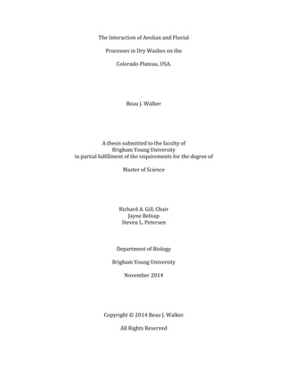
23. 19
7.
Figures
Figure
1
–
Deposition
and
erosion
of
aeolian
sediment
in
a
wash
at
Swing
Arm,
Factory
Butte,
UT.
A
(left)
show
the
wash
full
of
windblown
sediment,
and
B
(right)
shows
the
empty
wash
after
a
rain
event.
Photos
courtesy
Adam
Kind,
USGS
(Belnap
et
al.,
2011),
and
Beau
Walker.
A. B.

24. 20
Figure
2A
–
map
of
our
site
locations
across
the
Colorado
Plateau
from
Hanskville,
UT
to
Grand
Junction,
CO.
Nine
of
those
sites
also
had
game
cameras
(shown
by
circles
and
stars).
Of
those
nine,
three
also
had
weather
stations
installed
(shown
by
stars).
Figure
2B
–
Schematic
showing
our
typical
site
set
up.
We
had
eleven
sites
with
dust
traps
(buckets)
and
RTK
transects.

25. 21
Figure
3
–
Diagram
showing
the
general
process
for
creating
and
analyzing
3D
models
from
paired
images
(Matthews,
2008).
Image&&
Processing&
Point&Cloud&
Genera4on&
Change&
Detec4on&
Batch&processing&
of&images:&
• Ensure&proper&
digital&format&
• Remove&
8mestamp&
• Apply&any&
needed&image&
correc8ons&to&
all&images&
Agiso;&PhotoScan&
Python&Script:&
• Align&images&
• 3D&model&
crea8on&
• Export&xyz&
point&cloud&
Matlab&script:&
convert&point&
cloud&to&mesh.&
Align&meshes.&
Subtract&mesh&
from&one&
another.&Report&
difference&as&
percentage&
posi8ve&change.&&
Image&Set&1&H&3/24/11&12:00&PM& Image&Set&2&–&7/08/11&12:00&PM&

26. 22
A.
B.
Figure
4A.
Boxplot
showing
substrate
by
data
collection
period
(season)
deposition
in
upwind
dust
traps.
There
were
no
statistically
significant
differences.
Figure
4B.
Boxplot
showing
the
absolute
difference
between
upwind
and
downwind
dust
traps
by
data
collection
period
(season)
and
substrate.
12345678
logupwindsediment(g)
July 2012 October 2012 March 2013 June 2013
Mancos
Sand
log|upwind-downwind|sediment(g)
July 2012 October 2012 March 2013 June 2013
Mancos
Sand
-202468-202468

27. 23
Figure
5
–
Regression
tree
showing
the
variables
influencing
deposition
in
upwind
dust
traps.
R2 = 0.7854
310 g
95.5 g
759 g
226 g 2180 g
Disturbance =
Graze or Low
Disturbance =
OHV
Period = Jul‘12 - Jun ’13
Period = Mar‘12 - Jul ’12
n =34
n =23
n = 11
n = 8 n = 3

28. 24
Figure
6
–
Regression
tree
showing
the
variables
that
influence
the
difference
between
upwind
and
downwind
dust
traps.
R2 = 0.7249
∆ 153 g
∆ -24.8 g ∆ 524 g
∆ -178 g ∆ 42.3 g ∆ 151 g ∆ 1518 g
Disturbance =
Graze or Low
Disturbance =
OHV
Period = Jul
Period = Jun, Mar, Oct
Period = Jul‘12 - Jun ’13
Period = Mar‘12 - Jul ’12
n =34
n =23 n = 11
n = 7 n =16 n = 8 n = 3

29. 25
Figure
7
–
Regression
tree
showing
the
variables
that
influence
the
percent
positive
change
detected
by
game
cameras
in
all
three
washes
(sand
and
clay
substrates).
0.487
0.228
0.551
0.45 0.645
Precipitation
≥ 10.5 mm / w
Precipitation
< 10.5 mm / w
wind speed < 1.52 m/s
wind speed ≥ 1.52 m/s
n =33
n = 8
n = 25
n = 12 n = 13
R2 = 0.4767

30. 26
Figure
8
-­‐
Regression
tree
showing
the
variables
that
influence
the
percent
positive
change
detected
by
game
cameras
in
both
washes
with
clay
substrates.
49.7%
28.8 %
61.6 %
54.3 %
79.9 %
Precipitation ≥
10.5 mm / week
Precipitation <
10.5 mm / week
Period = Mar, Oct
Period = Jun, Jul
n = 22
n = 8
n = 14
n = 10
n = 4
R2 = 0.6314
VWC ≥ 0.06 m3/m3
VWC ≥ 0.06 m3/m3
47.6 %
n = 7
70.1 %
n = 3

31. 27
Table
1
–
Table
showing
detailed
site
characteristics
for
each
site.
Site%Nam
e
Latitiude
Longitude
Elevation%(m
)
Parent%M
aterial
Channel%W
idth%(m
)Channel%Depth%(m
)Channel%Flow
%Direction
Distance%to%w
eather%
station%(km
)W
eather%Station
%
%Plant%Cover
veg%type
Grazing%Level
Hank%A 38.26 L110.77 1,489 Mancos 1 1 NNE 3.2 HankB 10% ms medium
Hank%B 38.27 L110.80 1,463 Mancos 2 1 NNE 0 HankB 5% ss medium
Hank%C 38.27 L110.81 1,456 Mancos 2 1 NE 0.8 HankB 5% ss medium
Site%G 38.87 L109.85 1,405 Mancos 4 0.5 NNW 0 SiteG 10% ss heavy
Site%J 38.92 L109.43 1,340 Mancos 2 0.6 S 36.2 SiteG 20% ms medium
Site%K 38.91 L109.40 1,300 Mancos 1 1 S 39.9 SiteG 15% ss medium
Site%M 39.15 L108.54 1,504 Mancos 1 0.8 SW 4.3 GJ%Airport 20% ms ohv
average&for&Mancos&sites: 1.9 0.8 n/a 12.1 n/a 12% n/a n/a
Site%H 38.84 L110.03 1,320 Sandstone 3 1 W 15.6 SiteG 20% ms medium
Site%I 38.80 L110.06 1,292 Sandstone 1.4 0.7 NW 20.1 SiteG 20% ms medium
Site%L 38.56 L109.51 1,365 Sandstone 1.5 0.6 SW 0 SiteL 30% ts none
average&for&Sandstone&sites: 2 0.8 n/a 11.9 n/a 23% n/a n/a

32. 28
Period
Type
Mean
Sediment
Per
Bucket
(g)
Upwind
(g)
Downwind
(g)
U
-­‐
D
(g)
April
–
July
2012
Mancos
321.4
453.0
189.6
263.4
July
–
October
2012
Mancos
117.6
135.2
91.8
43.4
October
–
March
2013
Mancos
14.3
30.3
15.0
15.3
March
–
June
2013
Mancos
31.0
32.8
29.8
3
April
–
July
2012
Sand
1049.7
1293.1
806.2
486.9
July
–
October
2012
Sand
227.8
316.5
140.1
176.4
October
–
March
2013
Sand
105.9
184.4
35.7
148.7
March
–
June
2013
Sand
180.5
279.2
81.8
197.4
Table
2
–
Table
showing
mean
sediment
collected
by
dust
traps
during
each
collection
period.

33. 29
Table
3
–
Table
showing
data
from
RTK
transects
for
each
collection
period.
Site%Nam
e
Substrate
Period
∆%%in%w
ash%area%(m
2)
SiteM clay Jul%<%Oct
SiteG clay Oct%<%Mar <0.05232808
HankB clay Oct%<%Mar 0.20485
HankA clay Jul%<%Oct 0.227884862
SiteI sand Jul%<%Oct 0.74755
SiteI sand Oct%<%Mar <0.07625
SiteI sand Mar%<%Jun <0.06355

34. 30
Table
4
–
AIC
models
of
photogrammetry
data.
Model# Formula K AIC AICc ∆2AICc Step21 AICc2Weights2(wi)
1 gust&+&ws&+&log(precip&+&1) 3 27.75 28.5775862 3.7137931 0.1561565 0.032681053
2 gust&+&ws 2 25.95 26.3637931 1.5 0.47236655 0.098858747
3 gust&+&log(precip&+&1) 2 25.78 26.1937931 1.33 0.51427353 0.107629205
4 ws&+&log(precip&+&1) 2 25.79 26.2037931 1.34 0.51170858 0.107092402
5 tfv&+&log(precip&+&1) 2 25.74 26.1537931 1.29 0.52466254 0.109803459
6 gust&*&log(precip&+&1) 2 24.8 25.2137931 0.35 0.83945702 0.175684897
7 ws&*&log(precip&+&1) 2 25 25.4137931 0.55 0.75957212 0.158966269
8 tfv&*&log(precip&+&1) 2 24.45 24.8637931 0 1 0.209283969
Key
gust:&mean&gust&(m/s)&per&week&
ws:&mean&wind&speed&(m/s)&per&week
precip:&total&precip&(mm)&per&week&
tfv:&#&of&hours&per&week&with&average&wind&speeds&above&TFV