Information Gain

Note to other teachers and users of these slides.
Andrew would be delighted if you found this source
material useful in giving your own lectures. Feel free
to use these slides verbatim, or to modify them to fit
your own needs. PowerPoint originals are available. If
you make use of a significant portion of these slides in
your own lecture, please include this message, or the
following link to the source repository of Andrew’s
tutorials: http://www.cs.cmu.edu/~awm/tutorials .
Comments and corrections gratefully received.

Information Gain
Andrew W. Moore
Professor
School of Computer Science
Carnegie Mellon University
www.cs.cmu.edu/~awm
awm@cs.cmu.edu
412-268-7599

Copyright © 2001, 2003, Andrew W. Moore

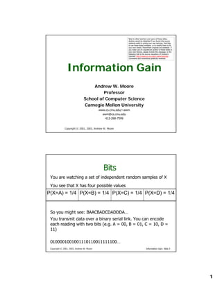
Bits
You are watching a set of independent random samples of X
You see that X has four possible values
P(X=A) = 1/4 P(X=B) = 1/4 P(X=C) = 1/4 P(X=D) = 1/4

So you might see: BAACBADCDADDDA…
You transmit data over a binary serial link. You can encode
each reading with two bits (e.g. A = 00, B = 01, C = 10, D =
11)

0100001001001110110011111100…
Copyright © 2001, 2003, Andrew W. Moore Information Gain: Slide 2

1

Fewer Bits
Someone tells you that the probabilities are not equal

P(X=A) = 1/2 P(X=B) = 1/4 P(X=C) = 1/8 P(X=D) = 1/8

It’s possible…

…to invent a coding for your transmission that only uses
1.75 bits on average per symbol. How?


Fewer Bits
Someone tells you that the probabilities are not equal

P(X=A) = 1/2 P(X=B) = 1/4 P(X=C) = 1/8 P(X=D) = 1/8

It’s possible…
…to invent a coding for your transmission that only uses
1.75 bits on average per symbol. How?
A 0
B 10
C 110
D 111

(This is just one of several ways)

2

Fewer Bits
Suppose there are three equally likely values…

P(X=A) = 1/3 P(X=B) = 1/3 P(X=C) = 1/3

Here’s a naïve coding, costing 2 bits per symbol

A 00
B 01
C 10

Can you think of a coding that would need only 1.6 bits
per symbol on average?

In theory, it can in fact be done with 1.58496 bits per
symbol.

General Case
Suppose X can have one of m values… V1, V2, … Vm

P(X=V1) = p1 P(X=V2) = p2 …. P(X=Vm) = pm
What’s the smallest possible number of bits, on average, per
symbol, needed to transmit a stream of symbols drawn from
X’s distribution? It’s
H ( X ) = − p1 log 2 p1 − p2 log 2 p2 − K − pm log 2 pm
m
= −∑ p j log 2 p j
j =1

H(X) = The entropy of X
• “High Entropy” means X is from a uniform (boring) distribution
• “Low Entropy” means X is from varied (peaks and valleys) distribution

3

General Case

P(X=V1) = p1 P(X=V2) = p2 …. P(X=Vm) = pm
A histogram of the
What’s the smallest possible number of frequency average, per
bits, on distribution of
symbol, needed to transmit a stream values of X would have
of symbols drawn from
A histogram of the
X’s distribution? It’s many lows and one or
frequency distribution of
two highs
H ( X ) = − p1 log 2would be flat 2 p2 − K − pm log 2 pm
values of X p − p log
1 2
m
= −∑ p j log 2 p j
j =1


General Case

P(X=V1) = p1 P(X=V2) = p2 …. P(X=Vm) = pm
A histogram of the
What’s the smallest possible number of frequency average, per
bits, on distribution of
symbol, needed to transmit a stream values of X would have
of symbols drawn from
A histogram of the
X’s distribution? It’s many lows and one or
frequency distribution of
two highs
H ( X ) = − p1 log 2would be flat 2 p2 − K − pm log 2 pm
values of X p − p log
1 2
m
= −∑ p ..and sop j values
j log 2 the ..and so the values
sampled from it would
j =1
sampled from it would
be all over the place be more predictable

4

Entropy in a nut-shell

Low Entropy High Entropy


Entropy in a nut-shell

Low Entropy High Entropy
..the values (locations of
..the values (locations soup) unpredictable...
of soup) sampled almost uniformly sampled
entirely from within throughout our dining room
the soup bowl

5

Specific Conditional Entropy H(Y|X=v)
Suppose I’m trying to predict output Y and I have input X
X = College Major Let’s assume this reflects the true
probabilities
Y = Likes “Gladiator”
E.G. From this data we estimate
X Y
• P(LikeG = Yes) = 0.5
Math Yes
History No • P(Major = Math & LikeG = No) = 0.25
CS Yes • P(Major = Math) = 0.5
Math No
• P(LikeG = Yes | Major = History) = 0
Math No
Note:
CS Yes
• H(X) = 1.5
History No
•H(Y) = 1
Math Yes

Definition of Specific Conditional
X = College Major
Entropy:
H(Y |X=v) = The entropy of Y
among only those records in which
X Y
X has value v
Math Yes
History No
CS Yes
Math No
Math No
CS Yes
History No
Math Yes

6

Definition of Specific Conditional
X = College Major
Entropy:
H(Y |X=v) = The entropy of Y
among only those records in which
X Y
X has value v
Math Yes
Example:
History No
CS Yes
• H(Y|X=Math) = 1
Math No
• H(Y|X=History) = 0
Math No
• H(Y|X=CS) = 0
CS Yes
History No
Math Yes

Conditional Entropy H(Y|X)
X = College Major Definition of Conditional
Entropy:

H(Y |X) = The average specific
X Y
conditional entropy of Y
Math Yes
= if you choose a record at random what
History No
will be the conditional entropy of Y,
CS Yes
conditioned on that row’s value of X
Math No
Math No = Expected number of bits to transmit Y if
CS Yes both sides will know the value of X
History No
= Σj Prob(X=vj) H(Y | X = vj)
Math Yes

7

Conditional Entropy
Definition of Conditional Entropy:
X = College Major
H(Y|X) = The average conditional
entropy of Y
= ΣjProb(X=vj) H(Y | X = vj)
X Y
Example:
Math Yes
History No vj Prob(X=vj) H(Y | X = vj)
CS Yes
Math 0.5 1
Math No
History 0.25 0
Math No
CS 0.25 0
CS Yes
History No
H(Y|X) = 0.5 * 1 + 0.25 * 0 + 0.25 * 0 = 0.5
Math Yes

Information Gain
Definition of Information Gain:
X = College Major
IG(Y|X) = I must transmit Y.
How many bits on average
would it save me if both ends of
the line knew X?
X Y
IG(Y|X) = H(Y) - H(Y | X)
Math Yes
History No
Example:
CS Yes
Math No • H(Y) = 1
Math No
• H(Y|X) = 0.5
CS Yes
• Thus IG(Y|X) = 1 – 0.5 = 0.5
History No
Math Yes

8

Information Gain Example


Another example


9

Relative Information Gain
Definition of Relative Information
X = College Major
Y = Likes “Gladiator” Gain:
RIG(Y|X) = I must transmit Y, what
fraction of the bits on average would
it save me if both ends of the line
X Y
knew X?
Math Yes
RIG(Y|X) = H(Y) - H(Y | X) / H(Y)
History No
CS Yes
Example:
Math No
H(Y|X) = 0.5
Math No •
CS Yes
H(Y) = 1
•
History No
Thus IG(Y|X) = (1 – 0.5)/1 = 0.5
•
Math Yes

What is Information Gain used for?
Suppose you are trying to predict whether someone
is going live past 80 years. From historical data you
might find…
•IG(LongLife | HairColor) = 0.01
•IG(LongLife | Smoker) = 0.2
•IG(LongLife | Gender) = 0.25
•IG(LongLife | LastDigitOfSSN) = 0.00001
IG tells you how interesting a 2-d contingency table is
going to be.

10

Information Gain

Recommended

Recommended

More Related Content

What's hot

What's hot (19)

Similar to Information Gain

Similar to Information Gain (20)

Recently uploaded

Recently uploaded (20)

Information Gain