This paper analyzes the error probability performance of different modulation schemes for orthogonal frequency division multiplexing (OFDM) based wireless local area network (WLAN) systems that follow the IEEE 802.11a standard. OFDM is used in WLANs to achieve high data rates and spectral efficiency. The performance of OFDM is evaluated for modulation schemes such as phase-shift keying, quadrature amplitude modulation, differential quadrature phase-shift keying, and offset quadrature phase-shift keying under additive white Gaussian noise. The bit error rate is compared against the signal-to-noise ratio for different modulation formats to determine the most suitable scheme for OFDM-based WLANs. OFDM has been adopted in


![Sanjeev Kumar, Swati Sharma
Error Probability of Different Modulation Schemes for OFDM
based WLAN standard IEEE 802.11a
Sanjeev Kumar sanjeev_be@indiatimes.com
Asst. Professor/ Electronics & Comm. Engg./
Amritsar college of Engg. & Technology, Amritsar,
143001, India
Swati Sharma swati.719@gmail.com
M.Tech Scholar/Electronics & Comm. Engg./
Amritsar college of Engg. & Technology, Amritsar,
143001, India
Abstract
Orthogonal Frequency Division Multiplexing (OFDM) is a key technique for
achieving high data rates and spectral efficiency requirements for wireless
communication systems. This paper presents a modeling and simulation of
OFDM based on WLAN standard (IEEE 802.11a). Performance of OFDM is
evaluated for different modulation schemes such as PSK, QAM, DQPSK, and
OQPSK. The performance of OFDM is compared in terms of BER vs SNR for
different modulation formats.
Keywords: Additive white Gaussian noise (AWGN), QAM, OQPSK, and DPSK.
1. INTRODUCTION
Wireless Local Area Networks (WLAN) and the exponential growth of the Internet have resulted
in an increased demand for new methods of obtaining high capacity wireless networks. OFDM is
a modulation scheme that allows digital data to be efficiently and reliably transmitted over a radio
channel, even in multipath environments [1, 2, 3]. In OFDM, the digital data is sent using many
carriers, each of a different frequency and these carriers are orthogonal to each other. All these
carriers transmit in unison using synchronized time and frequency, forming a single block of
spectrum. OFDM has found its application in a number of wireless and wireline systems. OFDM
has been adopted into several European wireless communications applications such as the
digital audio broadcast (DAB) and terrestrial digital video broadcast (DVB-T) systems [4, 5]. In the
United States, OFDM has been adopted in multipoint multichannel distribution services
(MMDS).Both wireless LAN applications-using standards such as IEEE 802.11a and the new
European Telecommunications Standard Institute’s (ETSI) HiperLAN/2 specification have also
installed OFDM as the modulation scheme[6,7].
Most WLAN systems currently use the IEEE802.11b standard, which provides a maximum data
rate of 11 Mbps. Newer WLAN standards such as IEEE802.11a and HiperLAN2 are based on
OFDM technology and provide a much higher data rate of 54 Mbps. However systems of the near
future will require WLANs with data rates of greater than 100 Mbps, and so there is a need to
further improve spectral efficiency and data capacity of OFDM systems in WLAN applications [8].
One of the main reasons for using OFDM for Wireless LANs is relatively small amount of delay
spread encountered in such applications [9].
International Journal of Engineering (IJE), Volume: 4, Issue: 4 262](https://image.slidesharecdn.com/ijev4i4-110103015036-phpapp02/75/International-Journal-of-Engineering-IJE-Volume-4-Issue-4-7-2048.jpg)
![Sanjeev Kumar, Swati Sharma
The paper presents the performance comparison results of the various digital modulation
techniques for OFDM in WLAN standard IEEE802.11a so as to obtain the most efficient
modulation technique for the same.
Digital data is transferred in an OFDM link by using a modulation scheme on each subcarrier. A
modulation scheme is a mapping of data words to a real (In phase) and imaginary (Quadrature)
constellation, also known as an IQ constellation. For example 64-QAM (Quadrature Amplitude
Modulation) has 64 IQ points in the constellation, constructed in a square with 8 evenly spaced
columns in the real axis and 8 rows in the imaginary axis. The number of bits that can be
transferred using a single symbol corresponds to log2 (M), where M is the number of points in the
constellation, thus 64-QAM transfers 6 bits per symbol. Each data word is mapped to one unique
IQ location in the constellation.
Differential Phase Shift Keying (DPSK) is the most common method of sending differential
information. Instead of mapping data to an absolute phase angle, as in the case of coherent
modulation, DPSK maps the data to a phase difference between symbols. For example, for
differential QPSK each symbol transmits 2 bits of information, corresponding to 4 different phase
differences.
2. OFDM GENERATION AND RECEPTION
OFDM signals are typically generated digitally. Figure 1 shows the block diagram of a typical
OFDM transceiver. The transmitter section converts digital data to be transmitted, into a mapping
of subcarrier amplitude and phase by using modulation techniques. It then transforms this
spectral representation of the data into the time domain using an Inverse Fast Fourier Transform
as it is much more computationally efficient, and so is used in all practical systems [10, 11]. The
addition of a cyclic prefix to each symbol solves both ISI and ICI [12, 13, 14]. If the channel
impulse response has a known length L, the prefix consists simply of copying the last L-1 values
from each symbol and appending them in the same order to the front of the symbol. Digital data is
then converted to serial form and transmitted over the channel.
After the time-domain signal passes through the channel, it is broken back into the parallel
symbols and the prefix is simply discarded. The receiver performs the reverse operation of the
transmitter. The amplitude and phase of the subcarriers is then picked out and converted back to
digital data.
FIGURE 1: Block diagram showing a basic OFDM transceiver
When an OFDM transmission occurs in a multipath radio environment, frequency selective fading
can result in groups of subcarriers being heavily attenuated, which in turn can result in bit errors.
International Journal of Engineering (IJE), Volume: 4, Issue: 4 263](https://image.slidesharecdn.com/ijev4i4-110103015036-phpapp02/75/International-Journal-of-Engineering-IJE-Volume-4-Issue-4-8-2048.jpg)

![Sanjeev Kumar, Swati Sharma
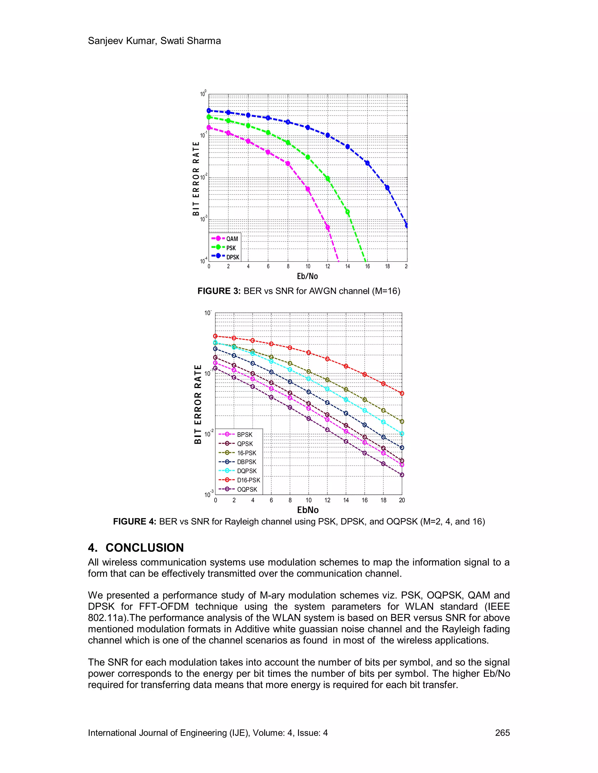
From the performed simulations, it was found that in AWGN channel, Coherent QAM performs
best in that it shows the least bit error rate requiring the least SNR for M=16 while differential PSK
is the worst for the same value of M. Whereas for M = 4, OQPSK performs the best as it requires
least SNR and DPSK performs the worst in AWGN channel.
Similarly, for Rayleigh channel, OQPSK modulation done on the transmitted bits performs the
best of all the other modulation techniques i.e. PSK and DPSK for the various values of M. The
low efficiency of PSK in AWGN channel is a result of under utilization of the IQ vector space. As it
is a known fact that PSK only uses the phase angle to convey information, with amplitude being
ignored, QAM uses both amplitude and phase for information transfer and so is more efficient
than PSK in AWGN channel for an OFDM system.
5. REFERENCES
[1] J. Chuang and N. Sollenberger, “Beyond 3G: Wideband wireless data access based on
OFDM and dynamic packet assignment,” IEEE Communications Mag., vol. 38, pp. 78–
87, July 2000.
[2] Saltzberg, B. R., “Performance of an Efficient Parallel Data Transmission System,” IEEE
Trans. on Communications, Vol. COM-15, No. 6, December 1967, pp. 805–811.
[3] A.G.Armada, “Understanding the Effects of Phase Noise in OFDM,” IEEE Transaction on
Broadcasting, vol. 47, No.2, June 2001.
[4] STOTT, J.H., “The DVB terrestrial (DVB-T) specification and its implementation in a
practical modem”. In proceedings of the 1996 International Broadcasting Convention,
IEEE Conference Publication No. 428, pp. 255-260, September 1996.
[5] Sari, Karam, Jeanclaude,“ Transmission techniques for digital terrestrial TV
broadcasting”, IEEE communications magazine Vol.33,No.2,Feb.1995.
[6] Ahmad R.S. Bahai and Burton R. Saltzberg. “Multicarrier digital communications, theory
and applications of OFDM”, Kluwer Academic Publishers, pp. 192 (2002)
[7] ETSI,“Hiperlan/2-TechnicalOverview”,Online:
http://www.etsi.org/technicalactiv/Hiperlan/hiperlan2tech.htm
[8] T. Pollet, M. van Bladen, and M. Moeneclaey, “BER sensitivity of OFDM systems to
carrier frequency offset and Wiener phase noise,” IEEE Trans. Commun., vol. 43, pp.
191–193, Feb./Mar./Apr. 1995.
[9] S. Glisic. “Advanced Wireless Communications, 4G Technology”. John Wiley & Sons Ltd:
Chichester, 2004.
[10] L. Hanzo, W. Webb, and T. Keller, “Single and Multi-carrier Quadrature Amplitude
Modulation”, New York, USA: IEEE Press-John Wiley, April 2000.
[11] S. B. Weinstein and P. M. Ebert, “Data transmission by frequency division multiplexing
using the discrete fourier transform,” IEEE Transactions on Communication Technology,
vol. COM–19, pp. 628–634, October 1971.
[12] K. Fazel and G. Fettweis, eds., “Multi-Carrier Spread-Spectrum”. Dordrecht: Kluwer,
1997. ISBN 0-7923-9973-0.
International Journal of Engineering (IJE), Volume: 4, Issue: 4 266](https://image.slidesharecdn.com/ijev4i4-110103015036-phpapp02/75/International-Journal-of-Engineering-IJE-Volume-4-Issue-4-11-2048.jpg)
![Sanjeev Kumar, Swati Sharma
[13] X. Cai and G. B. Giannakis, “Low-complexity ICI suppression for OFDM over time- and
frequency-selective Rayleigh fading channels,” in Proc. Asilomar Conf. Signals, Systems
and Computers, Nov. 2002.
[14] Shaoping Chen and Cuitao Zhu, “ICI and ISI Analysis and Mitigation for OFDM Systems
with Insufficient Cyclic Prefix in Time-Varying Channels” IEEE Transactions on
Consumer Electronics, Vol. 50, No. 1, February 2004.
[15] J.A.C. Bingham, “Multicarrier Modulation for Data Transmission: an idea who’s time has
come”, IEEE Communications Magazine, Vo1.28, No.5, pp.5-14, May 1990.
International Journal of Engineering (IJE), Volume: 4, Issue: 4 267](https://image.slidesharecdn.com/ijev4i4-110103015036-phpapp02/75/International-Journal-of-Engineering-IJE-Volume-4-Issue-4-12-2048.jpg)

![Dr. Krishpersad Manohar & Kimberly Ramroop
With the continued increase in design complexity and the modernization of process plant facilities,
the study of forced convection over cylindrical bodies has become an important one [1].
By the formulation of correlations, which consist of dimensionless parameters, such as Nusselt
number (Nu), Reynold’s number (Re) and Prandtl number (Pr), for different geometries, the values
of h can be calculated without having to analyze experimental data in every possible convective
heat transfer situation that occurs. Dimensionless numbers are independent of units and contain all
of the fluid properties that control the physics of the situation and involve one characteristic length.
It is advantageous to present data in the form of dimensionless parameters since it extends the
applicability of the data. However, correlations using dimensionless numbers are developed for
particular geometries and situations and are applicable within that range. Therefore, it is impractical
to use correlations developed for horizontal pipes to determine the h for inclined pipes.
2. PRESENTLY USED CORRELATIONS
Presently there are many correlations to predict the heat transfer from heated vertical or horizontal
pipes in both forced and natural convection situations. A review of literature on heat transfer
coefficients indicated that very little experimental work has been done on inclined pipes in the
recent past with little or no conclusive work reported for cross-flow pipe arrangement at various
angles of inclination. Generally, for design purposes cross flow correlations for horizontal pipes are
being used to determine heat transfer coefficients for inclined orientation. Few correlations exist for
inclined pipes with natural convection and none exist for inclined pipes in forced convection flow.
Following is a brief overview of the most common correlations that are being used for a horizontal
pipe in cross-flow.
2.1 Hilpert
Hilpert [2] was one of the earliest researchers in the area of forced convection from heated pipe
surfaces. He developed the correlation:
− 1
−
hD m (1)
Nu D = = C Re D Pr 3
k
TABLE I. HILPERT’S CONSTANTS FOR FORCED CONVECTION
ReD C m
0.4-4 0.981 0.33
4-40 0.911 0.385
40-4000 0.683 0.446
4000-400,000 0.193 0.618
400,000- 0.027 0.805
40,000,000
where the values of C and m, are given on Table I.
Hilpert’s calculations were done using integrated mean temperature values, not mean film
temperature values, and with inaccurate values for the thermophysical properties of air. The thermal
conductivity values of air used by Hilpert were lower (2-3%) than the most recent published results
[3]. This resulted in the values of Nusselt number calculated by the Hilpert correlation to be higher
than they should be.
International Journal of Engineering (IJE), Volume: 4, Issue: 4 269](https://image.slidesharecdn.com/ijev4i4-110103015036-phpapp02/75/International-Journal-of-Engineering-IJE-Volume-4-Issue-4-14-2048.jpg)
![Dr. Krishpersad Manohar & Kimberly Ramroop
2.2 Fand and Keswani
Fand and Keswani [4, 5] reviewed of the work of Hilpert and recalculated the values of the
constants C and m in equation 1 using more accurate values for the thermophysical properties of
air. The constants proposed by Fand and Keswani are given on Table II.
TABLE II. FAND’S CONSTANTS
ReD C m
1-4 - -
4-35 0.795 0.384
35-5000 0.583 0.471
5000-50000 0.148 0.633
50000-230000 0.0208 0.814
2.3 Zuakaukas
Another correlation proposed by Zukaukas [6] for convective heat transfer over a heated pipe was
0.25
Pr (2)
Nu f = c Re m Pr f0.37 f
f
Prw
where the values of c and m are given on Table III. Except for Prw, all calculations were done at the
mean film temperature.
TABLE III. ZUAKAUKAS’ CONSTANTS
ReD C m
1-40 0.76 0.4
40-103 0.52 0.5
103-2(10)5 0.26 0.6
2(10)5-107 0.023 0.8
2.4 Churchill and Bernstein
Churchill and Bernstein [7, 8] proposed a single comprehensive equation that covered the entire
range of ReD for which data was available, as well as a wide range of Pr. The equation was
recommended for all ReD.Pr > 0.2 and has the form
4
1
0.62 Re D2 + Pr
1
3 Re 8
5 5
Nu D = 0.3 + 1 + D
(3)
282,000
1
2
1 +
(0.4
Pr
) 3
4
This correlation was based on semi-empirical work and all properties were evaluated at the film
temperature.
2.5 Morgan
Morgan [9] conducted an extensive review of literature on convection from a heated pipe and
proposed the correlation
− 1
−
hD (4)
Nu D = = C Re m Pr 3
k
D
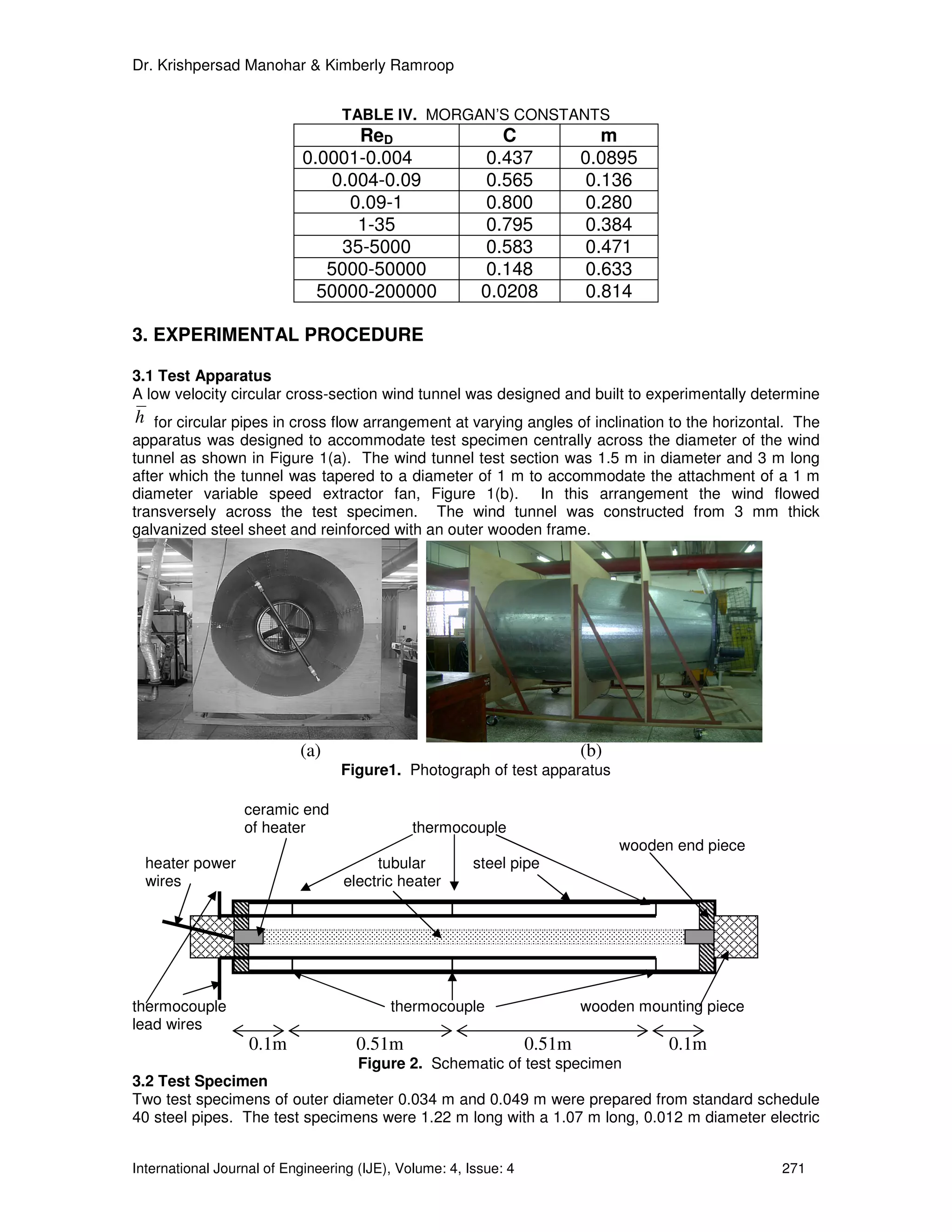
where the values of C and m are given on Table IV.
International Journal of Engineering (IJE), Volume: 4, Issue: 4 270](https://image.slidesharecdn.com/ijev4i4-110103015036-phpapp02/75/International-Journal-of-Engineering-IJE-Volume-4-Issue-4-15-2048.jpg)
![Dr. Krishpersad Manohar & Kimberly Ramroop
variation and the average of the three test results was calculated and used to determine the heat
transfer coefficient, h .
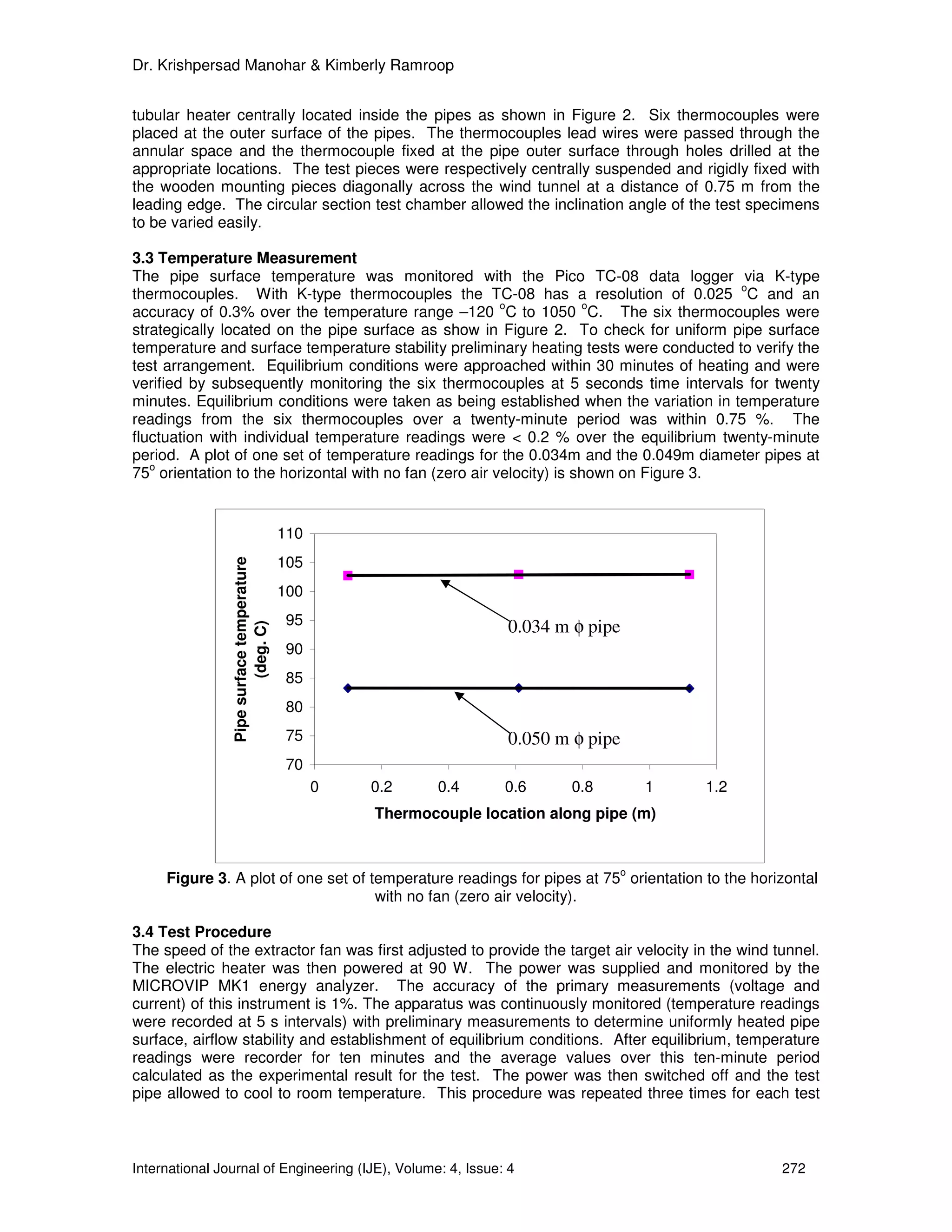
3.5 Tests Conducted
For the 0.034 m and the 0.049 m diameter pipes tests were conducted at 0, 15, 30, 45, 60, 75 and
90 degrees inclination to the horizontal for air flow velocities of 0.00 m/s, 0.80 m/s, 1.35 m/s and
2.50 m/s, for every case. For each test, after establishing equilibrium conditions, data for the pipe
surface temperature, wind tunnel wall temperature, ambient air temperature, wind speed across the
test specimen and power to the heater were recorded. The respective experimentally determined
heat transfer coefficient, h , was calculated for every case and the Nusselt number, Nu ,
determined.
4. CALCULATIONS
The measured power input to the heater was taken as the total heat loss from the pipe surface
under equilibrium conditions. The radiative heat loss component was calculated and the convective
heat loss component was then determined from equation (5). The average heat transfer coefficient,
h , was then calculated from the convective heat transfer component of equation (5).
(
Qtotal = Qconv + Qrad = h πDL(Ts − T∞ ) + εσπDL Ts4 − Tsurr
4
) (5)
The h was then used to determine the average Nusselt number, Nu , from equation (6).
h Do
Nu = (6)
k
Where Nu = average Nusselt number
2
h = average heat transfer coefficient (W/m K)
k = thermal conductivity of fluid (air) (W/m.K)
D0 = pipe outer diameter (m)
The Nu was also calculated for the corresponding test conditions with the commonly used
correlations of Hilpert, Fand and Keswani, Zukaukas, Churchill and Bernstein, and Morgan. The
calculated results are given on Table V.
4.1 Experimental Uncertainty
The experimental Nu was calculated from equation (6) using the experimentally determined h from
equation (5). The value of h depends on the measured power (voltage and current) and measured
temperature values. From equations (5) and (6) the relationship for the experimentally determined
Nu is given by equation (7).
Qtotal − Qrad 1 W − εσ (Ts4 − Tsurr ) 1
4
Nu = D = (7)
πDL(Ts − T∞ ) k πDL(Ts − T∞ ) k
From the theory of uncertainty analysis [10, 11]the uncertainty in experimentally determined Nusselt
∆Nu
number, , from the relation in equation (7) is given by equation (8)
Nu
International Journal of Engineering (IJE), Volume: 4, Issue: 4 273](https://image.slidesharecdn.com/ijev4i4-110103015036-phpapp02/75/International-Journal-of-Engineering-IJE-Volume-4-Issue-4-18-2048.jpg)


![Dharamvir Mangal, Devander Kumar Lamba, Tarun Gupta & Kiran Jhamb
4. CONCLUSION
This paper introduced the benefits of evacuated tube solar water heater. In India, it is still new model of
solar water heater which can be used in our household to face the challenge of climate change, global
warming, energy crisis etc.
5. REFERENCES
[1] G. L. Morrison, I. Budihardjo and M. Behnia. “Solar Energy”. 76 (1-3): 135-140, 2004
[2] I. Budihardjo, G.L. Morrison. “Solar Energy”. 83(1): 49-56, 2009
[3] G.L. Morrison, I. Budihardjo, M. Behnia. “Solar Energy”. 78 (2): 257-267, 2005
[4] “Fuel and Energy Abstracts”. 45 (4): 272, 2004
[5] “Fuel and Energy Abstracts”. 46 (6): 380, 2005
[6] G. L. Morrison, H. N. Tran. “Solar Energy”. 33(6):515-526, 198
[7] I. Budihardjo, G. L. Morrison, M. Behnia. “Solar Energy”. 81(12):1460-1472, 2007
International Journal of Engineering (IJE), Volume (4): Issue (4) 284](https://image.slidesharecdn.com/ijev4i4-110103015036-phpapp02/75/International-Journal-of-Engineering-IJE-Volume-4-Issue-4-29-2048.jpg)
![X.Felix Joseph, Dr.S.Pushpa Kumar, D.Arun Dominic & D.M.Mary Synthia Regis Prabha
density. Therefore, to realize high switching frequency in a converter changes its status (from on
to off), when the voltage across it and/or the current through it is zero at the switching instant.[3].
DC-DC converters are nonlinear systems due to their inherent switching operation. To assure a
constant output voltage, a classical linear design of a control is frequently used. The regulation is
normally achieved by the pulse width modulation (PWM) at a fixed frequency. The switching
device is a power MOSFET. The PWM linear control techniques are widely used [8].A number of
circuits [l], [2] and [5] use an additional switch to accomplish the function of soft switching the
main device. The circuits proposed in [2] and [4] use a single switch but the device count is high.
The circuit of accomplishes reduced voltage and current stresses and the coupling between main
and auxiliary circuit inductors significantly attenuate the duty cycle limitations [4].
The PI controller is proposed is to improve the performance of the soft switched boost converters.
The duty cycle of the boost converter is controlled by PI controller. The conventional PI
controllers for such converters are designed under the worst case condition of maximum load and
minimum line condition. As power electronic converters are nonlinear, and also are prone to
variations in its operating states over a wide range, the conventional PI controllers are to be
designed to provide optimal performance as the operating point changes. To provide optimal
performance at all operating conditions of the system PI controller is developed to control the duty
cycle of the boost converter. PI controller is designed based on an average state space model of
the classical boost DC-DC converter. Simulation of boost converter subjected to load changes is
performed to demonstrate the effectiveness of the proposed controller.[9][12]
A converter topology with single switch and switching strategies discussed in this paper, which
make the switch on at zero current and off at zero voltage at the given switching time. This
topology applied to a dc-dc boost converter. In this paper design and simulation of linear PI
controller for a soft switched dc-dc converter is discussed. The results were taken for different
load disturbances.
Design and Analysis of the Proposed Converter
FIGURE 1: Proposed Soft switched dc-dc boost converter
International Journal of Engineering (IJE), Volume: (4), Issue: (4) 286](https://image.slidesharecdn.com/ijev4i4-110103015036-phpapp02/75/International-Journal-of-Engineering-IJE-Volume-4-Issue-4-31-2048.jpg)
![X.Felix Joseph, Dr.S.Pushpa Kumar, D.Arun Dominic & D.M.Mary Synthia Regis Prabha
The circuit diagram of the proposed converter with soft switching scheme is shown in fig.1, the
switch S1, L1, D3 and C2 are the main boost converter components, while R represents the
resistive load on the converter. Inductor L2, L3, D1, D2 and C1 form the auxiliary circuit for
accomplishing the soft switching of S1. Inductors L2 and L3 are much smaller than L1 and C1 is
much smaller than C2. There are seven modes of operation. The duration of modes 1, 2, 5 and 6
being quite small iL1 and Vout are assumed constant at I1 and V1 for modes 1 and 2, and I2 and V2
for modes 5 and 6 respectively.[10]
MODE 1: This mode begins with the turn on of S1, at zero current at t 0 .The expressions are,
V1
i L2 (t ) = t (1)
L2
vC1 (t ) = [V1 − VC1 (t 0 )][1 − cos ω1t ] + VC1 (t 0 ) (2)
sin ω1t
i L3 (t ) = [VC1 (t 0 ) − V1 ] (3)
ω1 L3
1
Where ω1 =
L3 C1
When D3 stops conducting and this mode comes to an end.
MODE 2: The initial conditions on L3, L2 and C1 are, i L3 (t1 ) , i L2 (t1 ) + I 1 and VC1 respectively,
attained at the end of
Mode 1.The expressions are,
i L3 (t1 )
VC1 (t ) = −VC1 (t1 )[1 − cos ω 2 t ] + sin ω 2 t − VC1 (t 0 ) (4)
ω 2 C1
VC1 (t1 )
i L3 (t ) = sin ω 2 t + i L3 (t1 ) cos ω 2 t (5)
ω 2 ( L2 + L3 )
VC1 (t1 )
i L2 (t ) = sin ω 2 t + i L3 (t1 ) cos ω 2 t + I 1 (6)
ω 2 ( L 2 + L3 )
1
Where ω2 =
( L 2 + L 3 )C 1
This mode comes to an end when VC1 reaches zero at t2.
MODE 3: The initial conditions on i L2 , i L3 and VC1 for this mode i L2 (t 2 ), i L3 (t 2 ) are zero The
expression for i L3 is,
V S L2
i L3 (t ) = − t + I L3 (t 2 ) (7)
L1 L2 + L2 L3 + L3 L1
This mode comes to an end at t 3 when i L3 reaches zero at t 3 .
MODE 4: In this mode current buildup in L1 and L2, and Vout(t) are governed by the equations as
follows.
International Journal of Engineering (IJE), Volume: (4), Issue: (4) 287](https://image.slidesharecdn.com/ijev4i4-110103015036-phpapp02/75/International-Journal-of-Engineering-IJE-Volume-4-Issue-4-32-2048.jpg)
![X.Felix Joseph, Dr.S.Pushpa Kumar, D.Arun Dominic & D.M.Mary Synthia Regis Prabha
VS
i L1 (t ) = i L2 (t ) = t + I1 (8)
L1 + L2
1
RC 2
Vout (t ) = V1e (9)
This mode comes to an end when S1 is turned off at zero voltage at t4 .
MODE 5: This mode begins with the turn off of S1 at zero voltage at t4.The expressions are,
I2
VC1 (t ) = V2 (1 − cos ω 3 t ) + sin ω 3 t (10)
ω 2 C1
L2
I L2 (t ) = [V2 C1 sin ω 3t − I 2 (1 − cos ω 3 t )] + I 2 (11)
( L2 + L3 )
L2
I L3 (t ) = [ −V2 C1ω 3 sin ω 3 t + I 2 (1 − cos ω 3 t )] (12)
( L2 + L3 )
1
Where ω3 =
L2 L3
C1
L2 + L3
This mode ends when i L2 reaches zero at t6 .
MODE 6: In this mode i L3 reduces to zero. This mode comes to an end at t6 when i L3 becomes
zero. The expression for i L3 and VC1 for these mode is.
VC1 (t 5 ) − V2
i L3 = sin ω1t + i L3 (t 5 ) cos ω1t (13)
L3ω1
i L3 (t 5 )
VC1 (t ) = [VC1 (t 5 ) − V2 ][cos ω1t − 1] sin ω1t (14)
ω1C1
MODE 7: In this mode iL2, iL3 are zero. This mode comes to an end at t7 when S1 is turned on at
zero current. This is the normal mode of the boost converter. The expressions are,
Vout (t ) = e −αt [ A sin ω 4 t + B sin ω 4 t ] + VS (15)
Vout (t) −αt
iL1 (t) = + e [(−BC2 + AC2ω4t) cosω4t − ( AC2 + BC2ω4 ) sinω4t] (16)
R
1 1
Where α= , ω4 =
2 RC 2 L1C 2
I2 V2 α (V2 − V5 )
A= − +
ω 4 C 2 Rω 4 C 2 ω4
B = V2 − V S
International Journal of Engineering (IJE), Volume: (4), Issue: (4) 288](https://image.slidesharecdn.com/ijev4i4-110103015036-phpapp02/75/International-Journal-of-Engineering-IJE-Volume-4-Issue-4-33-2048.jpg)


![X.Felix Joseph, Dr.S.Pushpa Kumar, D.Arun Dominic & D.M.Mary Synthia Regis Prabha
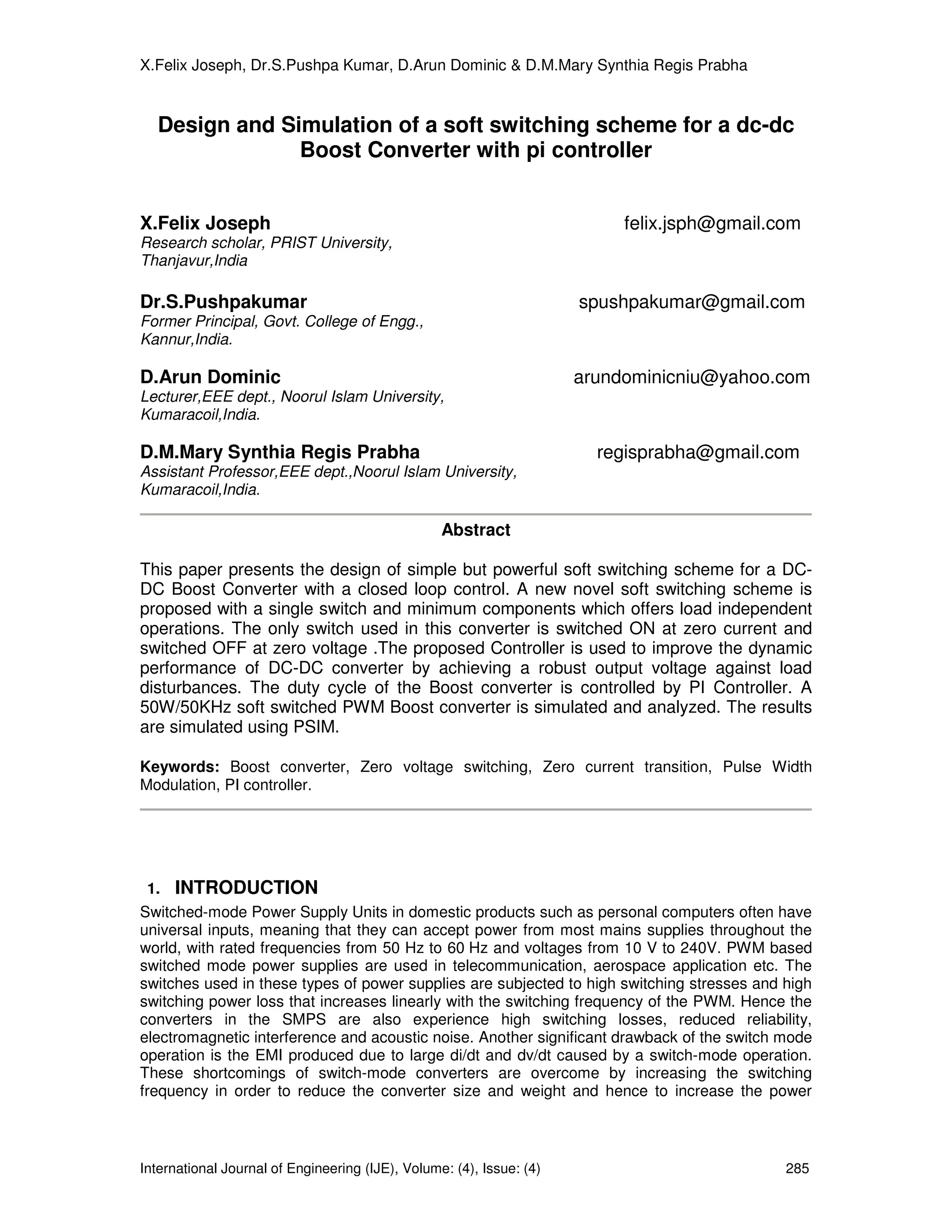
FIGURE 6: Zero Voltage waveform of the Soft switched dc-dc boost converter
FIGURE 7: Output Voltage waveform of the proposed converter with PI controller Vout=150V
3. COMPARATIVE EVALUATION
Many researchers [13][14] explained soft switched dc –dc boost converter with two
switches which gives high switching losses, in that one switch act as soft switching and the other
as hard switching. The comparative evaluation of our results with the other research work shows
that the total harmonic distortion is reduced as much as possible. Fig.8 clearly shows that the
total harmonic distortion of soft switched dc-dc converter with two switches have fundamental and
other odd harmonics.
Fig.9 shows that the total harmonic distortion of our proposed soft switched dc-dc converter with
a single switch. It is clearly seen from the fig.9, except fundamental harmonics, higher order
harmonics are eliminated, which gives the improved results over the other research works. In
future we will eliminate the fundamental harmonics by using a suitable filter design techniques.
International Journal of Engineering (IJE), Volume: (4), Issue: (4) 292](https://image.slidesharecdn.com/ijev4i4-110103015036-phpapp02/75/International-Journal-of-Engineering-IJE-Volume-4-Issue-4-37-2048.jpg)


![Lyes Khezzar & Saleh M. Al-Alawi
of the expansion plane are important topics of consideration for design of fluidic devices, heat-
exchangers and mixing systems.
It is known that laminar flow downstream of a sudden expansion remains symmetric with two
equal separation zones on either side of the centerline of the duct for low Reynolds numbers.
However, beyond a critical value of the Reynolds number the flow becomes asymmetric,
producing two or three unequal separation zones. The exact underlying phenomenon is still not
well understood but is thought to be due to a Coanda like phenomenon and the appearance of
asymmetric flow is thought to coincide with a bifurcation of the Navier-Stokes equations. It has
been found both experimentally and numerically that the value of the critical Reynolds number
beyond which the flow behavior becomes asymmetric is dependent on the expansion ratio. Of
particular interest in these flows, is the variation of reattachment lengths with Reynolds number
and expansion ratio.
Plane sudden expansion flows have been investigated experimentally by Durst et al [1], Cherdron
et al [2] and Fearn et al. [3]. These investigations included flow visualisation and fluid velocity
measurements by laser Doppler anemometry. Numerical investigations were also conducted by
Durst et al [1], Fearn et al [3] and Battaglia et al [4]. The techniques used were generally based
on time integration by finite difference/element techniques of the incompressible form of the
Navier-Stokes equations. The calculations of these flows with mesh sizes necessary to resolve
the flow field, provide grid-independent solutions and to obtain the salient features of the flow for
every Reynolds number can be very time consuming. For example, using a Computational Fluid
Dynamic (CFD) commercial code, around 27 hours of computing time on a SUN-20 workstation,
are necessary to obtain a converged solution for a single Reynolds number.
ANNs are computer models that are trained in order to recognize both linear and non-linear
relationships among the input and the output variables in a given data set. In general, ANN
applications in engineering have received wide acceptance. The popularity and acceptance of
this technique stems from its features, which are particularly attractive for data analysis. These
features include handling of fragmented and noisy data, speed inherent to parallel distributed
architectures, generalization capability over new data, ability to effectively incorporate a large
number of input parameters, and its capability of modeling non-linear systems. In general, ANN
models consists of three basic elements: an organized architecture of interconnected processing
elements, a method for encoding information during training, and a method for recalling
information during testing. Simpson (1990) provides a coherent description of these elements
and presents comparative analyses, applications, and implementation of 27 different ANN
paradigms. This tool can be used by mechanical engineers in conjunction with other analytical
and graphical techniques for data analysis, optimisation and model evaluation.
When considering the reattachment length of sudden-expansions the judicious combination of
CFD calculated solutions with ANN will result in a considerable saving in computing and
turnaround time. Thus CFD can be used in the first instance to obtain reattachment lengths for a
limited choice of Reynolds numbers and ANN will be used subsequently to predict the
reattachment lengths for other intermediate Reynolds number values.
The purpose of this work is twofold. First present a CFD analysis of flows through plane sudden
expansions. Second, the results of this analysis will be used in conjunction with ANN to
demonstrate that the hybrid combination of ANN and CFD modelling allows a considerable time
saving in the prediction of reattachment lengths for plane sudden expansions.
The next section of this paper will present the theoretical model used to obtain finite-volume
solutions to the flow through plane sudden expansions chosen from previously published work.
Section three presents the ANN model, the results are presented in section 4 followed by
conclusions.
International Journal of Engineering (IJE), Volume (4): Issue (4) 297](https://image.slidesharecdn.com/ijev4i4-110103015036-phpapp02/75/International-Journal-of-Engineering-IJE-Volume-4-Issue-4-42-2048.jpg)
![Lyes Khezzar & Saleh M. Al-Alawi
2. NUMERICAL SIMULATION IN PLANE SYMMETRIC SUDDEN EXPANSIONS
2.1 Model Equations and Numerical Method
The flow is assumed to be laminar, two-dimensional and unsteady, the fluid viscous and
incompressible. Under these assumptions, the continuity and momentum equations are therefore
written in their conservative form and for Cartesian systems of co-ordinates as:
∂U ∂V
+ =0 (1)
∂x ∂y
+
( )
∂(U ) ∂ U 2 ∂(UV )
+ =−
1 ∂P µ ∂ 2U ∂ 2U
+ + (2)
∂t ∂x ∂y ρ ∂x ρ ∂x 2 ∂y 2
∂(V ) ∂(UV ) ∂ V
+ +
2
=−
( )
1 ∂P µ ∂ V ∂ V
+
2
+
2
(3)
∂t ∂x ∂y ρ ∂y ρ ∂x 2 ∂y 2
where, (U, V) are the fluid velocity vector Cartesian components, P represents the pressure and
ρ and µ the density and viscosity of the fluid respectively.
The finite-volume technique is used to solve the above equations. The second order QUICK
scheme of Leonard [5] was employed for the discretization convection fluxes and a second-order
centred difference scheme was adopted for diffusive fluxes. The pressure field P is solved with
the PISO algorithm, see Issa [6]. Temporal integration is achieved through a fully implicit
-5
formulation with a time step of 10 . Convergence was assumed when the global rates of change
-10 -11 -7
of the variables were between 10 and 10 for laminar flow and 10 for turbulent flow and
monitoring of variables at relevant positions in the flow field. All the calculations were carried on
a SUN-20 workstation, to 64-bits precision.
2.2 Initial-boundary conditions and meshes
The geometrical details of the configuration are shown on figure 1. The computational grid was
rectangular and extended from the exit plane of the expansion to a downstream position giving a
length of up to 70 step-heights.
The calculations proceeded by impulsively starting the flow from rest. At the inlet boundary, a
fully developed parabolic profile was prescribed.
At the outlet plane, a zero gradient condition is enforced for all variables and this boundary was
located at a downstream distance of 50 and in some instances 70 step heights. The axial length
of the domain of integration was assumed to be long enough to capture the flow details and
remove upstream influence of the outlet boundary face value. At solid boundaries, the usual law
of the wall was used.
The mesh was rectangular with uniform distributions along the stream wise and cross-stream
directions. Three grid sizes were used 150×55 and 200×93 and 250×110 to generate grid
independent solutions as judged by the profiles of the axial velocity. There were no significant
differences between the results of the last two grids and therefore the intermediate one was
adopted in all the computations.
International Journal of Engineering (IJE), Volume (4): Issue (4) 298](https://image.slidesharecdn.com/ijev4i4-110103015036-phpapp02/75/International-Journal-of-Engineering-IJE-Volume-4-Issue-4-43-2048.jpg)
![Lyes Khezzar & Saleh M. Al-Alawi
Xr1
Recirculation zones
d D
Xr2
Xr3
Xr4
FIGURE 1: Geometrical configuration of the plane sudden-expansion.
3. ARTIFICIAL NEURAL NETWORKS MODEL
3.1 Artificial Neural Networks
An artificial neural network (ANN) method is a computational mechanism able to acquire,
represent, and compute a mapping from one multivariate space of information to another, given a
set of data representing that mapping. ANNs have the ability to mimic the human brain as well as
their ability to learn and respond [7]. This technique found wide acceptance in various
engineering applications since they have proven to be effective in performing complex operations,
process and functions in a variety of fields.
An ANN can be considered as a collection of numerous simple processors organised in layers
called neurons or nodes. These nodes are the basic organizational units of a neural network that
are arranged in a series of layers to create the ANN by unidirectional communication channels
(connections) that carry numerical data. Nodes are classified as input, output, or hidden layer
nodes depending on their location and function within the network see Stern [8]. Data is received
from sources external to the neural network through the input layer nodes, while data is
transmitted out of the neural network through the output layer nodes. Hidden layer neurons act
as the computational nodes in the neural network, communicating between input nodes and other
hidden layer or output nodes. The number of nodes in the input layer is equal to the number of
independent variables entered into the network which represent the input parameters whereas
the number of output nodes corresponds to the number of variables to be predicted. The number
of hidden layers and nodes used within the hidden layer vary according to the complexity of the
task the network must perform see DeTienne et al.[9].
3.2 Model Development
It has been clearly established that the reattachment length for laminar flow depends on two non-
dimensional parameters, the Reynolds number and the expansion ratio (E.R.=D/d). This
dimensional analysis relationship forms the basis of the Artificial Neural Network model which is
developed below.
Thus, an ANN model was developed for predicting reattachment positions for the expansion
ratios of 2, 3 and 5. The ANN Architecture for this model is shown in Figure 2. The model
consists of three layers, an input layer, a hidden layer and an output layer. The neurones in the
input layer receive two input representing the Reynolds number (Re) and the Expansion ratios
(E.R.); hence, two neurones were used for input in the ANN architecture. The output layer, on
the other hand, consists of four neurones representing the reattachment positions (Xr1, Xr2, Xr3,
and Xr4 of figure 1). The single hidden layer used consisted of 5 neurones. The initial number
International Journal of Engineering (IJE), Volume (4): Issue (4) 299](https://image.slidesharecdn.com/ijev4i4-110103015036-phpapp02/75/International-Journal-of-Engineering-IJE-Volume-4-Issue-4-44-2048.jpg)
![Lyes Khezzar & Saleh M. Al-Alawi
of nodes used in the single hidden layer was calculated using the equation developed by
Carpenter and Hoffman [10]:
N = η[H ( I + 1) + n( H + 1)]] (4)
Input Layer Hidden Layer Output Layer
Xr1
Xr2
3 R
e
Xr3
Xr4
FIGURE 2: The Architecture for the Developed ANN Model.
Where, η is a constant greater than 1.0 (i.e. η =1.25 would give a 25% over-determined
approximation, N the number of training pairs available, H the number of hidden nodes to be
used in the network with one hidden Layer, I and n the number of input and output nodes
respectively.
The result obtained using equation (4) indicated that four hidden nodes could be used in the
hidden layer to develop the ANN architecture. However, the best result for the model was found
with eight nodes in the hidden layer. Research in this area by Lapeds and Forber [11] and
Hecht-Nielsen [12] proved that one or two hidden layers with an adequate number of neurones is
sufficient to model any solution surface of practical interest
4. RESULTS
4.1 CFD results
The results of the CFD simulations are presented first. A detailed comparison with measured
velocity data is conducted so as to provide the necessary confidence in other predicted flow
parameters such as reattachment lengths for other values of Reynolds number.
The experimental results of Fearn et al. [3] are used in the study of the velocity profiles
predictions. The heights of the upstream and downstream ducts were 4 and 12 mm respectively
and the area and aspect ratios 1:3 and 8:1 respectively. Below a Reynolds number of 60, the
flow was found to be symmetric.
Figure 3 illustrates detailed comparison of the calculated axial velocity profiles and their
experimental counter parts, as measured by Fearn et al. [3], for several downstream positions for
a Reynolds number equal to 187. The agreement between the calculated and measured profiles
is excellent. The profile inside the third recirculation zone is also accurately predicted.
International Journal of Engineering (IJE), Volume (4): Issue (4) 300](https://image.slidesharecdn.com/ijev4i4-110103015036-phpapp02/75/International-Journal-of-Engineering-IJE-Volume-4-Issue-4-45-2048.jpg)
![Lyes Khezzar & Saleh M. Al-Alawi
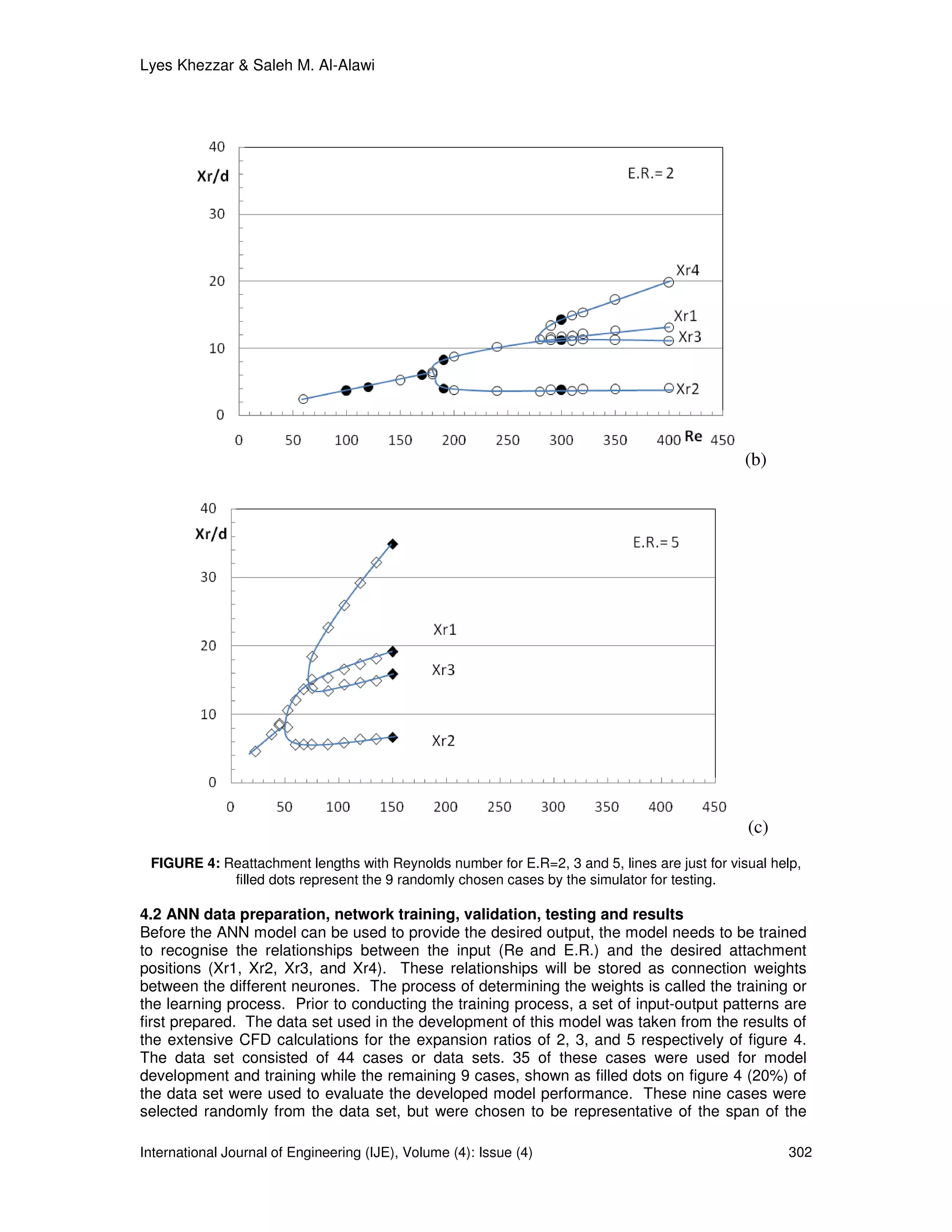
Figure 4 shows the predicted reattachment lengths with Reynolds number for the three expansion
ratios of 2, 3 and 5. They correspond to the experimental studies and configurations of Cherdron
et al [2], Fearn et al [3] and Ouwa et al [13]. The reattachment location is determined as the
position where the stream wise velocity is zero at the first grid point from the wall. The trend of all
the three curves reveals a symmetric flow at low values of the Reynolds number and transition to
asymmetric flow occurs at a critical value of the latter. Initially, only two recirculation zones are
present with a third one appearing later. The part of the curves that corresponds to symmetric
flow extrapolates to a finite recirculation length at zero Reynolds number. Ouwa et al. [13]
reported variations of the two first reattachment lengths (Xr1 and Xr2) with Reynolds number and
their results agree remarkably well with the present calculations. The inferred values of the
critical Reynolds number for the three ratios of 2, 3 and 5 are 180, 60 and 45 respectively and
compare well with the experimental values of 185, 54 and 45. The source of the discrepancies is
difficult to trace but can be explained in terms of difficulty in obtaining an exact value for the
transitional Reynolds number.
x/h=2.5
1.0
x/h=10
x/h=20
x/h=40
0.5
U/U0
0.0
0 2 4 6 8 10 12
Y (mm)
FIGURE 3: Axial Mean velocity (Fearn et al), Re=187.
(a)
International Journal of Engineering (IJE), Volume (4): Issue (4) 301](https://image.slidesharecdn.com/ijev4i4-110103015036-phpapp02/75/International-Journal-of-Engineering-IJE-Volume-4-Issue-4-46-2048.jpg)
![Lyes Khezzar & Saleh M. Al-Alawi
Reynolds numbers at hand and the three expansion ratios. The multi-layer feed-forward network
used in this work was trained using the Back-propagation (BP) paradigm developed by
Rumelhart and McClelland [14]. Simpson [15] gives a different equation that provides a
generalised description of how the learning and recall process is performed by the BP algorithm.
The training process of this ANN model was performed using the NeuroShellTM simulator. After
-5
completing 180429 epoch, the network converged to a threshold of 10 . The network model
2 2
goodness of fit, R (R is defined as the coefficient of determination), demonstrated that the
developed ANN model produced attachment positions that were in close agreement with the
2
actual values. The R values of the outputs Xr1, Xr2, Xr3, and Xr4 were 0.8617, 0.8325, 0.9397
and 0.9682 respectively. Having trained the network successfully, the next step is to test the
network’s generalisation capability using a different data set in order to judge its performance.
Using the 9 cases that were randomly selected from the data set, the developed model was
2
tested to assess its generalisation capabilities. The R values for the Xr1, Xr2, Xr3, and Xr4
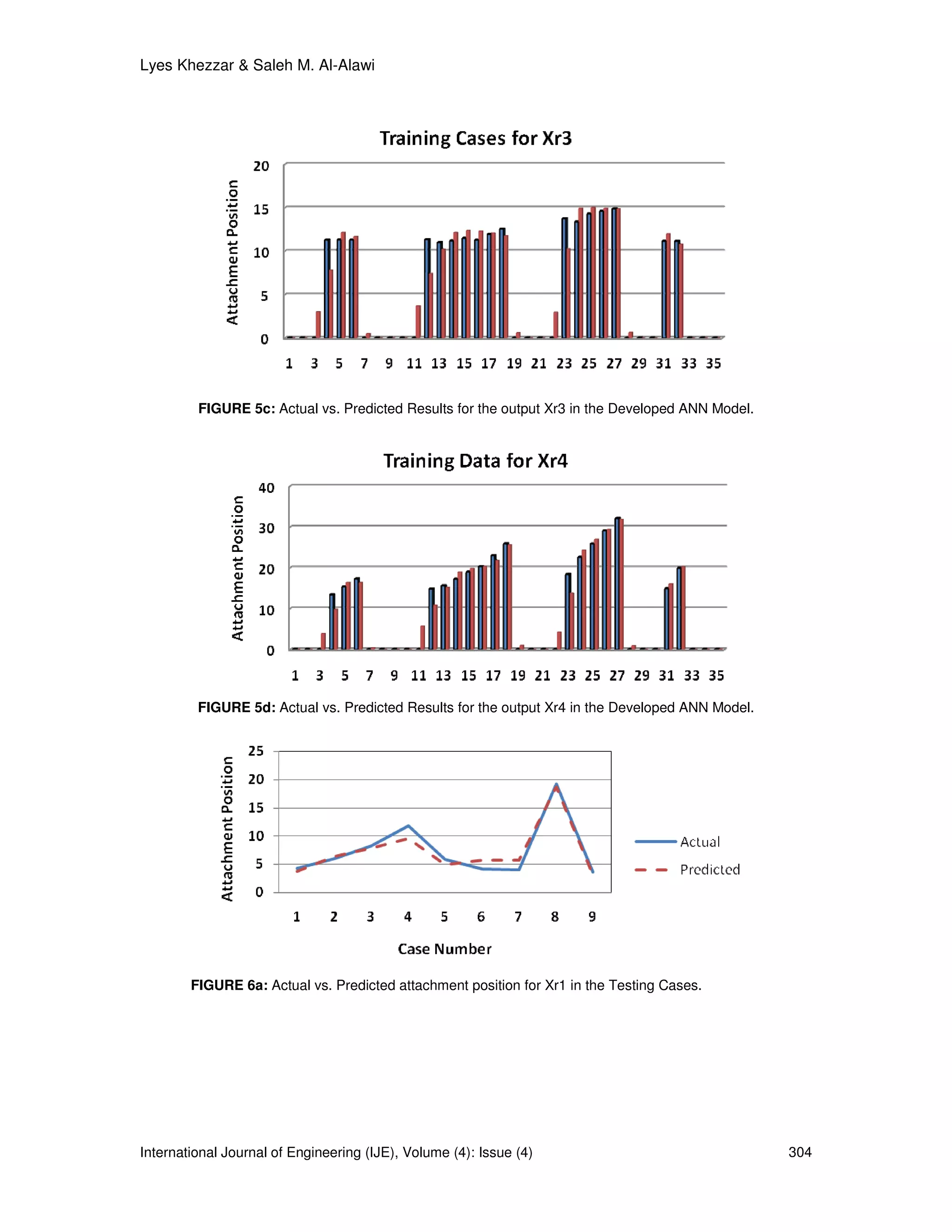
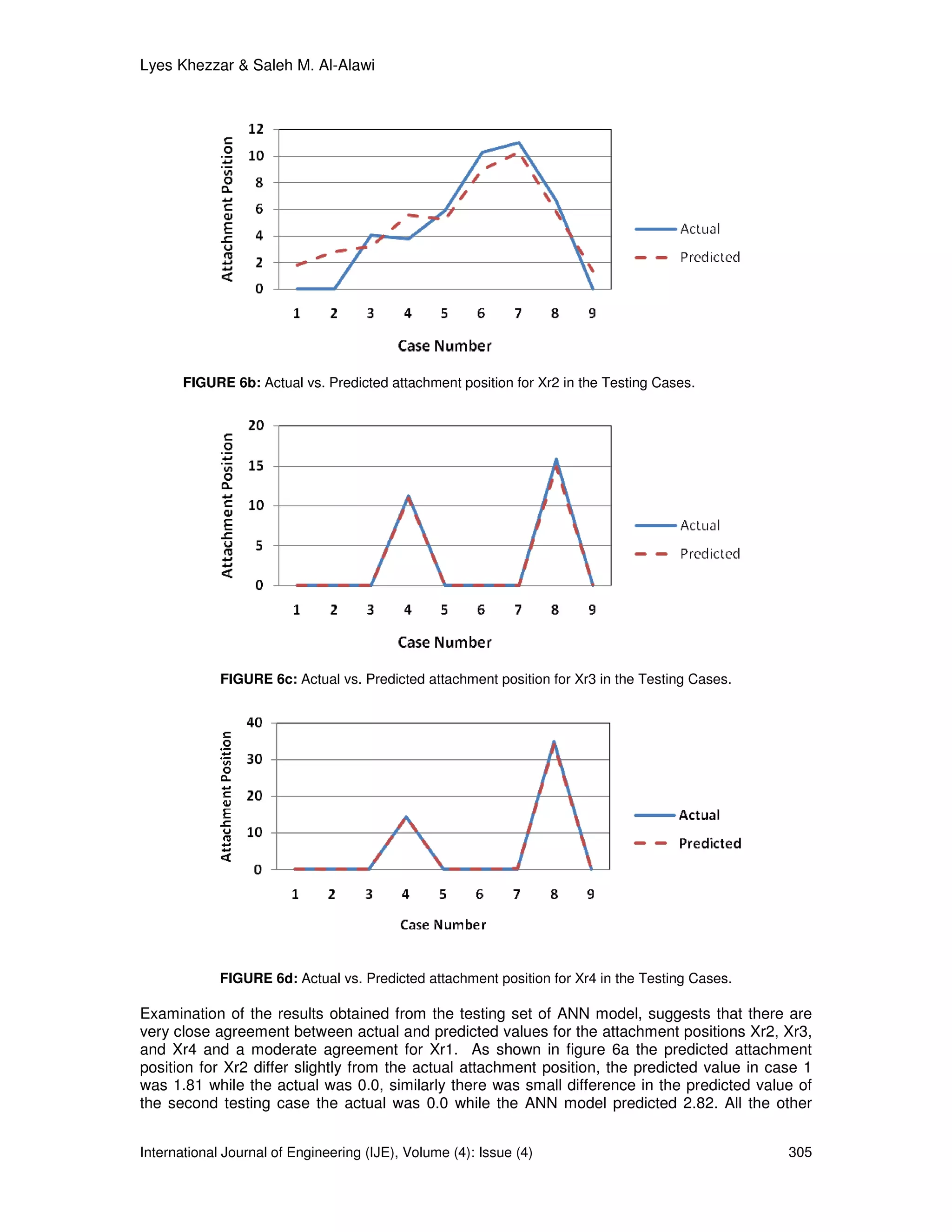
were 0.9383, 0.8577, 0.997 and 0.999 respectively. Figures 5(a, b, c, d) and 6 (a, b, c, d)
illustrate the relationship between actual and predicted attachment positions of Xr1, Xr2, Xr3,
and Xr4 for the training data and the testing data sets respectively.
FIGURE 5a: Actual vs. Predicted Results for the output Xr1 in the Developed ANN Model.
FIGURE 5b: Actual vs. Predicted Results for the output Xr2 in the Developed ANN Model.
International Journal of Engineering (IJE), Volume (4): Issue (4) 303](https://image.slidesharecdn.com/ijev4i4-110103015036-phpapp02/75/International-Journal-of-Engineering-IJE-Volume-4-Issue-4-48-2048.jpg)

![Zahra Faeli, Ali Fakher & Seyed Reza Maddah Sadatieh
Allowable Differential Settlement of Oil Pipelines
Zahra Faeli afs_faeli@yahoo.com
Researcher/ Faculty of Civil Engineering
University of Tehran Tehran,
1779816691,Iran.
Ali Fakher afakher@ut.ac.ir
Associate Professor / Faculty of Civil Engineering
University of Tehran Tehran,
1779816691,Iran.
Seyed Reza Maddah Sadatieh srmaddah@ut.ac.ir
Assistant Professor / Faculty of Engineering Science
University of Tehran Tehran,
1779816691,Iran.
Abstract
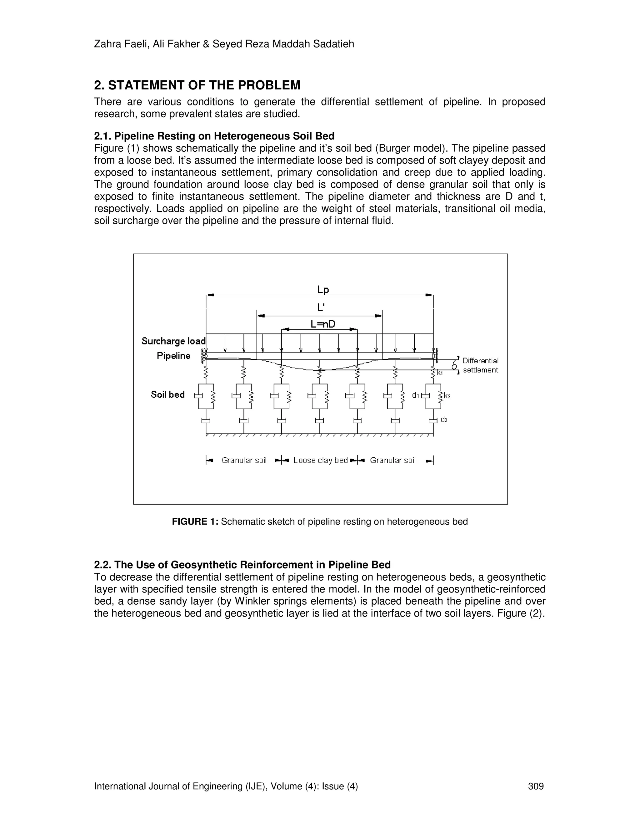
The allowable settlement of pipelines has been mentioned rarely in design
references and codes. The present paper studies the effects of differential
settlement of pipeline bed on resulted forces and deformations and then
determines the allowable differential settlement of pipelines in two conditions as
follows: (i) heterogeneous soil bed and (ii) adjacent to steel tanks. To accomplish
the studies, numerical simulation of pipeline is used. The pipeline bed is idealized
by Winkler springs and four-element standard viscoelastic Burger model. Also,
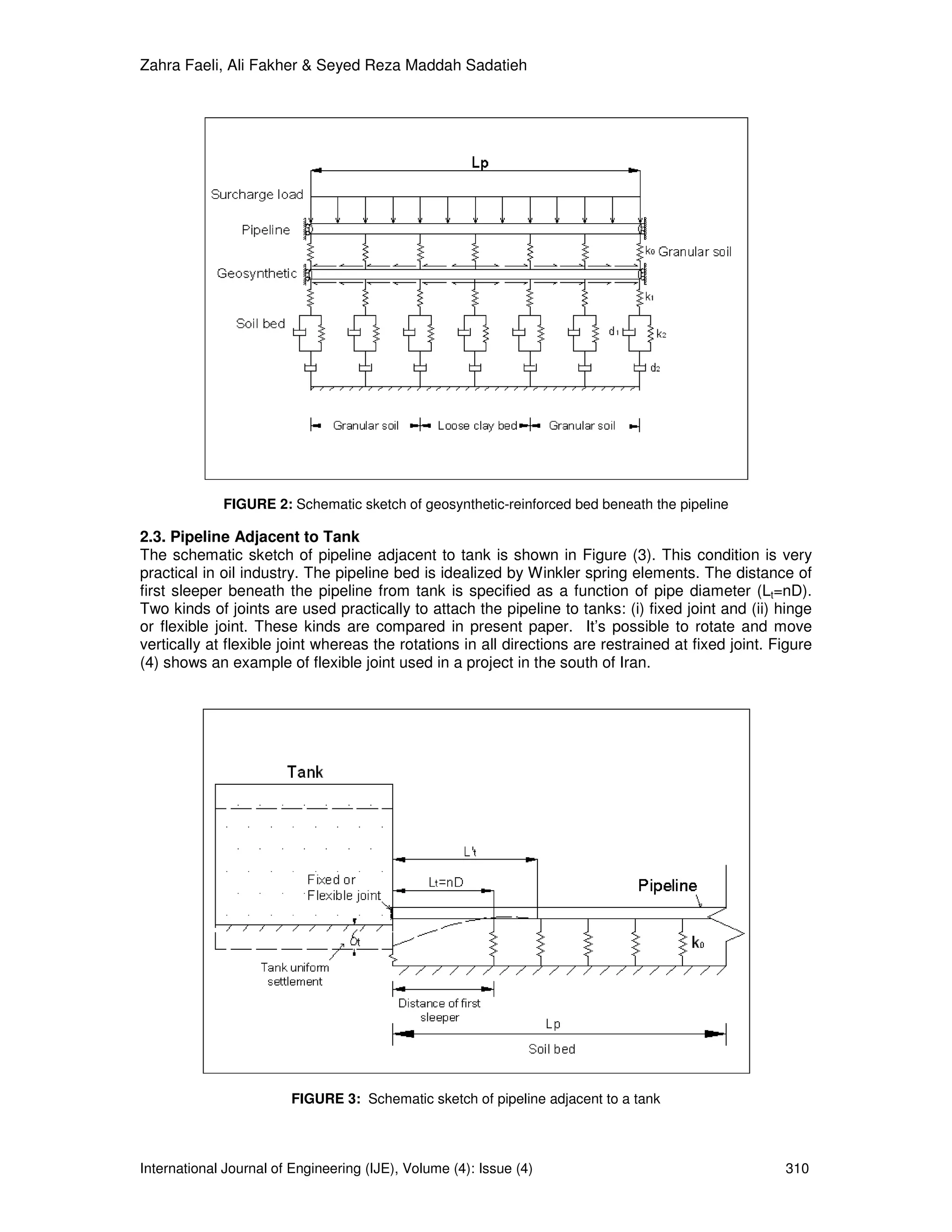
the use of geosynthetic reinforcement is studied in heterogeneous soil beds and
the effect of geosynthetics on decreasing the settlement is investigated. The
pipeline-tank joints in two cases of fixed and flexible joints are investigated and
the results for two kinds of joints are compared.
Keywords: Allowable differential settlement, Burger model, Fixed joint, Flexible joint, Geosynthetic.
1. INTRODUCTION
The values of allowable settlement of pipeline have been discussed rarely in pipeline design
references and this subject has been challenged geotechnical and pipeline engineers.
Discussions about allowable settlement of pipelines were propounded for pipelines constructed in
permafrost zone and exposed to thaw differential settlement [1] & [2]. Also, investigations have
been proposed about evaluation of deformations and generated forces of pipelines exposed to
settlement of soil bed [3] & [4] . Moreover, studies to analysis the deformations of pipeline due to
settlement of other equipments were accomplished [5]. But such a comprehensive study has yet
not been made to determine the quantitative and qualitative values of allowable differential
settlement of pipelines.
International Journal of Engineering (IJE), Volume (4): Issue (4) 308](https://image.slidesharecdn.com/ijev4i4-110103015036-phpapp02/75/International-Journal-of-Engineering-IJE-Volume-4-Issue-4-53-2048.jpg)
![Zahra Faeli, Ali Fakher & Seyed Reza Maddah Sadatieh
Tank
Pipeline
FIGURE 4: Pipeline-tank flexible joint
3. NUMERICAL SIMULATION USED IN RESEARCH
A computer program had been written in ABAQUS [6] finite element software to carry out the
studies.
3.1. Simulation of Soil Bed by Burger Model
Idealization of structures beds by lumped parameter elements (spring elements) is considerable
in previous investigations [7] but there are few references about the subject of Burger model
used in soil beds [8]. This model idealizes primary and secondary (creep) consolidations as well
as instantaneous settlement. Each Burger model element is consisted of two spring elements
with k1 and k2 stiffness coefficients and two dashpot elements with d1 and d2 viscous coefficients.
The behavior of Burger element exposed to the force of F and resulted deflection of y is stated as
equation (1):[9]
(1)
3.2. Pipeline Structure Model
The pipeline is idealized by three dimensional PIPE31 elements in present analyses and the pipe
cross sections are selected according to the sections of API-5L-95 code [10] to use standard
sections. The hoop stress (σh) and equivalent stress (σe) are defined as relations (2) and (3),
respectively:[11]
(2)
(3)
Where P= internal pressure, D and t= diameter and thickness of pipeline respectively, σl=
longitudinal stress and τ=shear stress of cross section. To study the effect of pipeline diameter,
the ratio of diameter to thickness (D/t) is considered to be constant approximately in amount of
64.
International Journal of Engineering (IJE), Volume (4): Issue (4) 311](https://image.slidesharecdn.com/ijev4i4-110103015036-phpapp02/75/International-Journal-of-Engineering-IJE-Volume-4-Issue-4-56-2048.jpg)
![Zahra Faeli, Ali Fakher & Seyed Reza Maddah Sadatieh
3.3. Geosynthetic Model
To idealize geosynthetic layer, T3D2 tensile elements are used. To consider frictional strength of
between the geosynthetic layer and granular soil (confinement effect) a distributed tensile force is
applied over the geosynthetic layer as equation (4).
(4)
Where Tg= distributed tensile force, f= frictional coefficient (considered in amount of 1), γs= soil
3
density (20 kN/m ) and H=height of soil (1m).
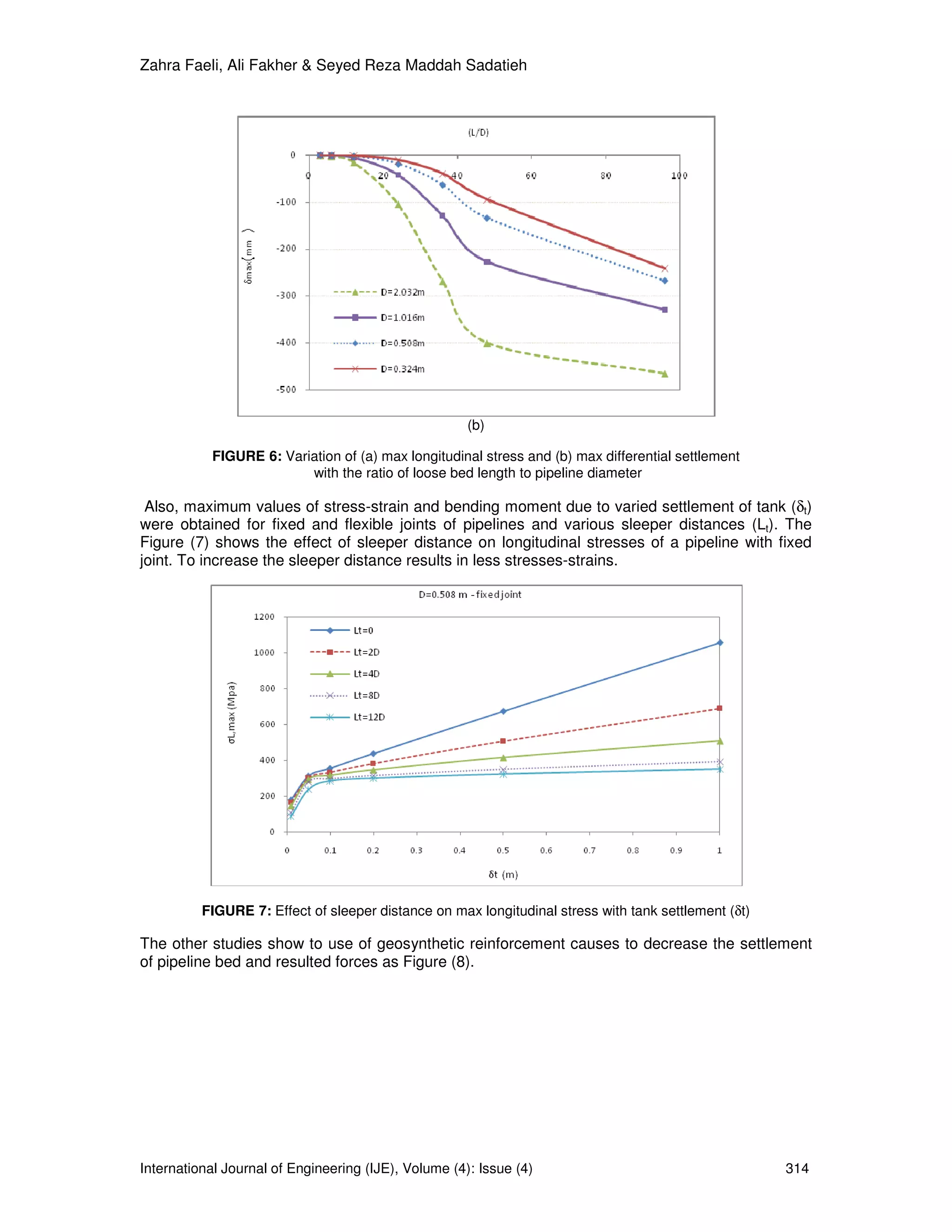
4. THE EFFECTS OF VARIABLES
The effects of variables of Burger model on the values of settlement and resulted forces of
pipeline were studied. The stiffness coefficient of spring element as series in Burger model (and
stiffness coefficient of Winkler model) is determined by the relation of subgrade reaction modulus
according to plate-load test [12]. The spring element of Burger model as series is used to model
the instantaneous settlement of bed (relation 5) :
( ) (5)
Where D= plate width (pipe diameter), Li=element length (0.01m), µ=Poisson’s ratio of soil (0.5)
and E=elasticity module of soil.
To vary the stiffness ratio of dense granular soil to intermediate loose clay soil (k1(g)/k1(c)) in
heterogeneous soil bed showed the differential settlements have increased till k1(g)/k1(c)=25 and
then varied negligibility. Hence, in present study the ratio of k1(g)/k1(c) is considered to be 25.The
studies showed to select the coefficients of k2, d1 and d2 as very large for around dense soil
resulted in only instantaneous settlement. These variables for intermediate loose clay soil were
determined so that maximum long term settlement would be arised in various amounts of loose
bed lengths. In this way, minimum values are obtained for allowable settlement of pipelines on
heterogeneous beds.
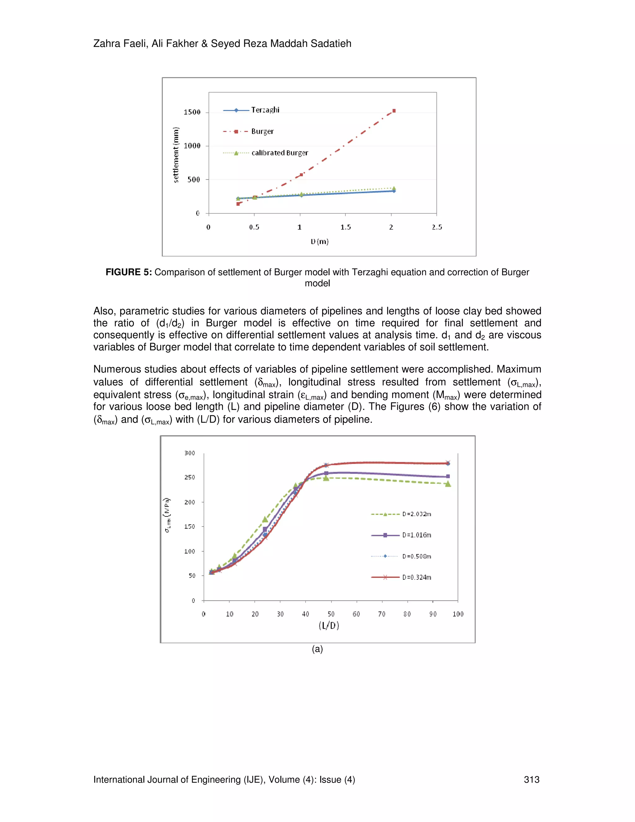
The studies showed k2=k1/100 resulted in maximum long term settlement of pipeline. The variable
of k2 in equation (1) is used to model the primary consolidation settlement. The primary
consolidation values of bed due to various pipeline loads were obtained from used Burger model
and Terzaghi relation as Figure (5). To compare the settlements of Burger model with Terzaghi
relation resulted in calibrated parameter of Burger model (k2) that is stated as equation (6). This
relation is used to determine the variable of k2 for various diameters of pipelines. The settlements
resulted from Burger model with calibrated variable of k2 are in good agreement with settlements
calculated by Terzaghi relation as Figure (5).
( ) (6)
International Journal of Engineering (IJE), Volume (4): Issue (4) 312](https://image.slidesharecdn.com/ijev4i4-110103015036-phpapp02/75/International-Journal-of-Engineering-IJE-Volume-4-Issue-4-57-2048.jpg)
![Zahra Faeli, Ali Fakher & Seyed Reza Maddah Sadatieh
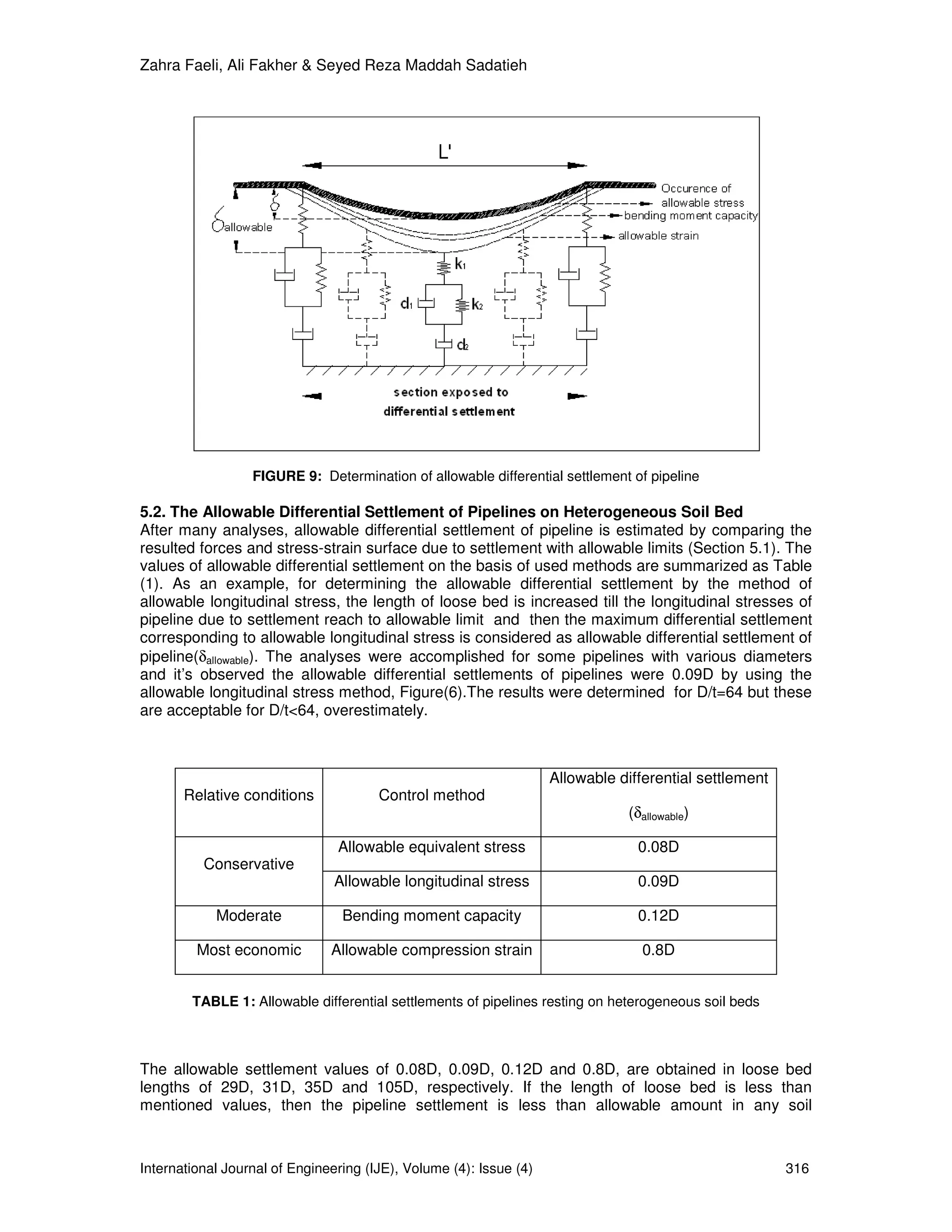
FIGURE 8: The effects of geosynthetic layer on differential settlement of pipeline
with the ratio of loose bed length to pipeline diameter (L/D)
5. DISCUSSION ABOUT ALLOWABLE SETTLEMENT OF PIPELINES
5.1. The Criteria for Limiting the Settlement
The present paper aim is to suggest allowable differential settlement of pipelines. To limit the
settlement, various criteria could be used. Stress and strain are two main criteria for limiting the
pipeline settlement. Historically, the most codes of pipelines have used the allowable stress-
based design methods to design the pipelines against applied forces. In the half of the ’90 ies
limit state design methods entered the pipeline design codes. In this way, to define failure states
of pipelines has provided the possibility of more efficient and economic designs. The limit state
design methods use limited strains and bending moments moreover the limited stresses.
(i). Allowable stress method:
For this method in present research the design factors were used from ABS2000 code [13]. This
code limits the hoop stresses, longitudinal and equivalent stresses to 72%, 80% and 90%
specified minimum yield stress (SMYS), respectively.
(ii). Bending moment capacity method:
The bending moments of pipeline were controlled by this method. Maximum allowable bending
moment of pipeline (MAllowable) is determined according to the proposed relation of reference [14].
(iii). Allowable strain method:
The critical compression strain of pipeline materials ( ) would be estimated by using empirical
equation according to CSA-Z662 code [15]. The limit state of plastic failure of welds is initiated
from the cracks of weld surface due to tensile strains. Many of codes consider the value of 2% as
allowable tensile strain [16].
As settlement increases, the above mentioned three criteria would happen respectively. See
Figure (9).
International Journal of Engineering (IJE), Volume (4): Issue (4) 315](https://image.slidesharecdn.com/ijev4i4-110103015036-phpapp02/75/International-Journal-of-Engineering-IJE-Volume-4-Issue-4-60-2048.jpg)