Downloaded 19 times

![Linear Search – Recursive Code
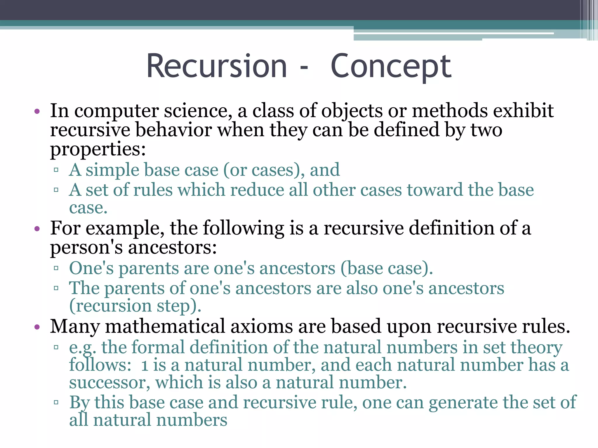
int linearSearch(const int list[], int first, int last, int
key)
{
if (first == last) // base case: target not found
return last;
if (list[first] == target) // base case: target found
return first;
// inductive step: search with range [first+1, last)
return RecLinearSearch (arr, first+1, last, target)
} // end RecLinearSearch](https://image.slidesharecdn.com/week3-recursionandsorting-191013065809/75/Recursion-and-Sorting-Algorithms-19-2048.jpg)
![Binary Search W & W/O Recursion
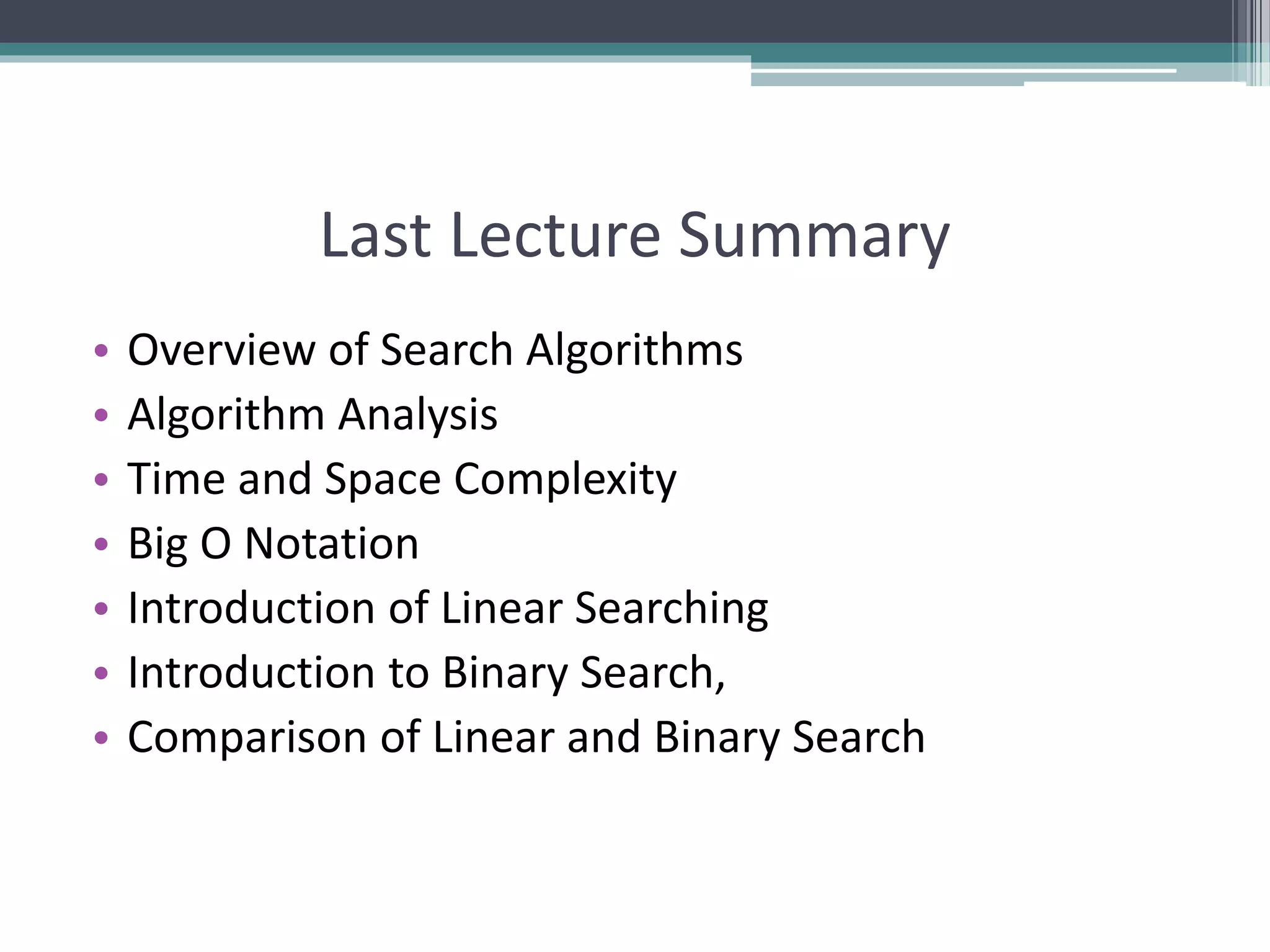
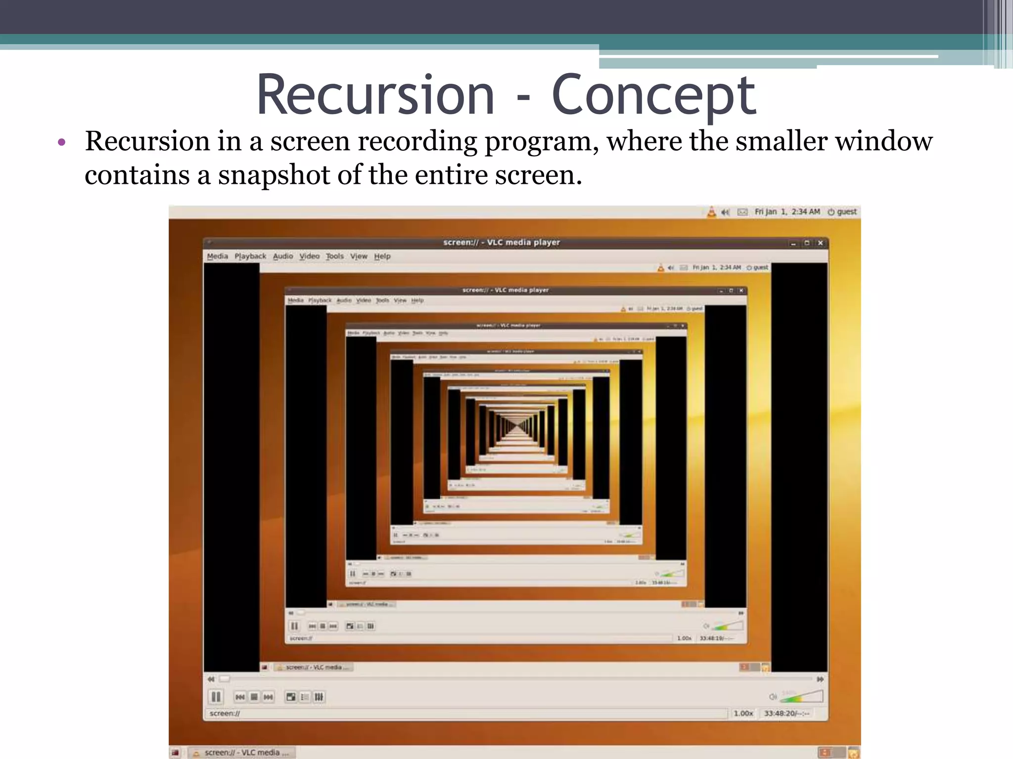
int first, last, upper;
first = 0;
last = size - 1;
while (true) {
middle = (first + last) / 2;
if (data[middle] == value)
return middle;
else if (first >= last)
return -1;
else if (value < data[middle])
last = middle - 1;
else
first = middle + 1;
}
}
{ int middle = (first + last) / 2;
if (data[middle] == value)
return middle;
else if (first >= last)
return -1;
else if (value < data[middle])
return bsearchr(data, first, middle-1, value);
else
return bsearchr(data, middle+1, last, value);
}
w/o recursion
with recursion](https://image.slidesharecdn.com/week3-recursionandsorting-191013065809/75/Recursion-and-Sorting-Algorithms-20-2048.jpg)
![Basic Terminology
• Internal sort
▫ When a set of data to be sorted is small enough such that
the entire sorting can be performed in a computer’s
internal storage (primary memory)
• External sort
▫ Sorting a large set of data which is stored in low speed
computer’s external memory such as hard disk, magnetic
tape, etc.
• Ascending order
▫ An arrangement of data if it satisfies “less than or equal to
<=“ relation between two consecutive data
▫ [1, 2, 3, 4, 5, 6, 7, 8, 9]](https://image.slidesharecdn.com/week3-recursionandsorting-191013065809/75/Recursion-and-Sorting-Algorithms-33-2048.jpg)
![Basic Terminology
• Descending order
▫ An arrangement of data if it satisfies “greater than or equal to
>=“ relation between two consecutive data
▫ e.g. [ 9, 8, 7, 6, 5, 4, 3, 2, 1]
• Lexicographic order
▫ If the data are in the form of character or string of characters and
are arranged in the same order as in dictionary
▫ e.g. [ada, bat, cat, mat, max, may, min]
• Collating sequence
▫ Ordering for a set of characters that determines whether a
character is in higher, lower or same order compared to another
▫ e.g. alphanumeric characters are compared according to their
ASCII code
▫ e.g. [AmaZon, amaZon, amazon, amazon1, amazon2]](https://image.slidesharecdn.com/week3-recursionandsorting-191013065809/75/Recursion-and-Sorting-Algorithms-34-2048.jpg)
![Basic Terminology
• Random order
▫ If a data in a list do not follow any ordering mentioned above,
then it is arranged in random order
▫ e.g. [8, 6, 5, 9, 3, 1, 4, 7, 2]
▫ [may, bat, ada, cat, mat, max, min]
• Swap
▫ Swap between two data storages implies the interchange of
their contents.
▫ e.g. Before swap A[1] = 11, A[5] = 99
▫ After swap A[1] = 99, A[5] = 11
• Item
▫ Is a data or element in the list to be sorted.
▫ May be an integer, string of characters, a record etc.
▫ Also alternatively termed key, data, element etc.](https://image.slidesharecdn.com/week3-recursionandsorting-191013065809/75/Recursion-and-Sorting-Algorithms-35-2048.jpg)
![Basic Terminology
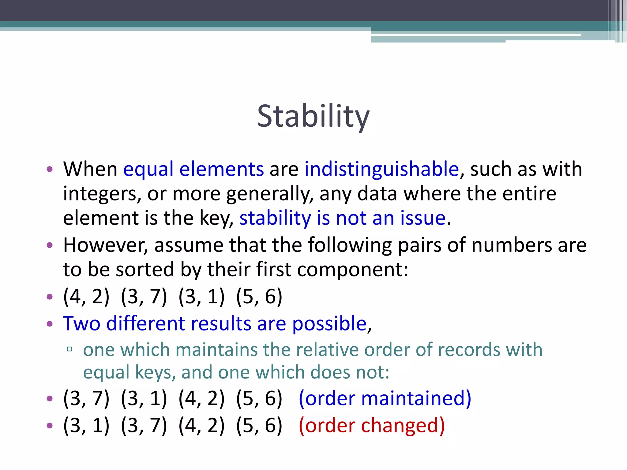
• Stable Sort
▫ A list of data may contain two or more equal data. If a
sorting method maintains the same relative position of
their occurrences in the sorted list then it is stable sort
▫ e.g. [ 2, 5, 6, 4, 3, 2, 5, 1, 5 ]
▫ [ 1, 2, 2, 3, 4, 5, 5, 5, 6 ]
• In Place Sort
▫ Suppose a set of data to be sorted is stored in an array A
▫ If a sorting method takes place within the array A only, i.e.
without using any other extra storage space
▫ It is a memory efficient sorting method](https://image.slidesharecdn.com/week3-recursionandsorting-191013065809/75/Recursion-and-Sorting-Algorithms-36-2048.jpg)


![0
10
20
30
40
50
60
70
[1] [2] [3] [4] [5] [6]
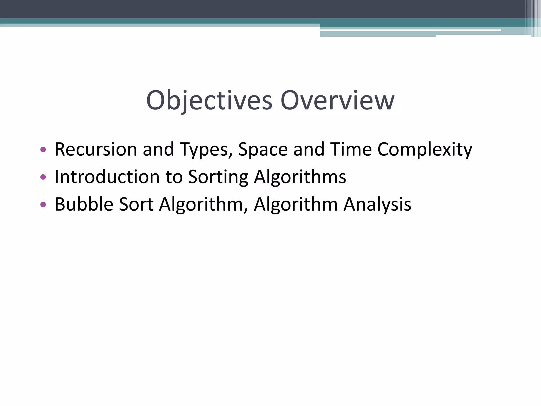
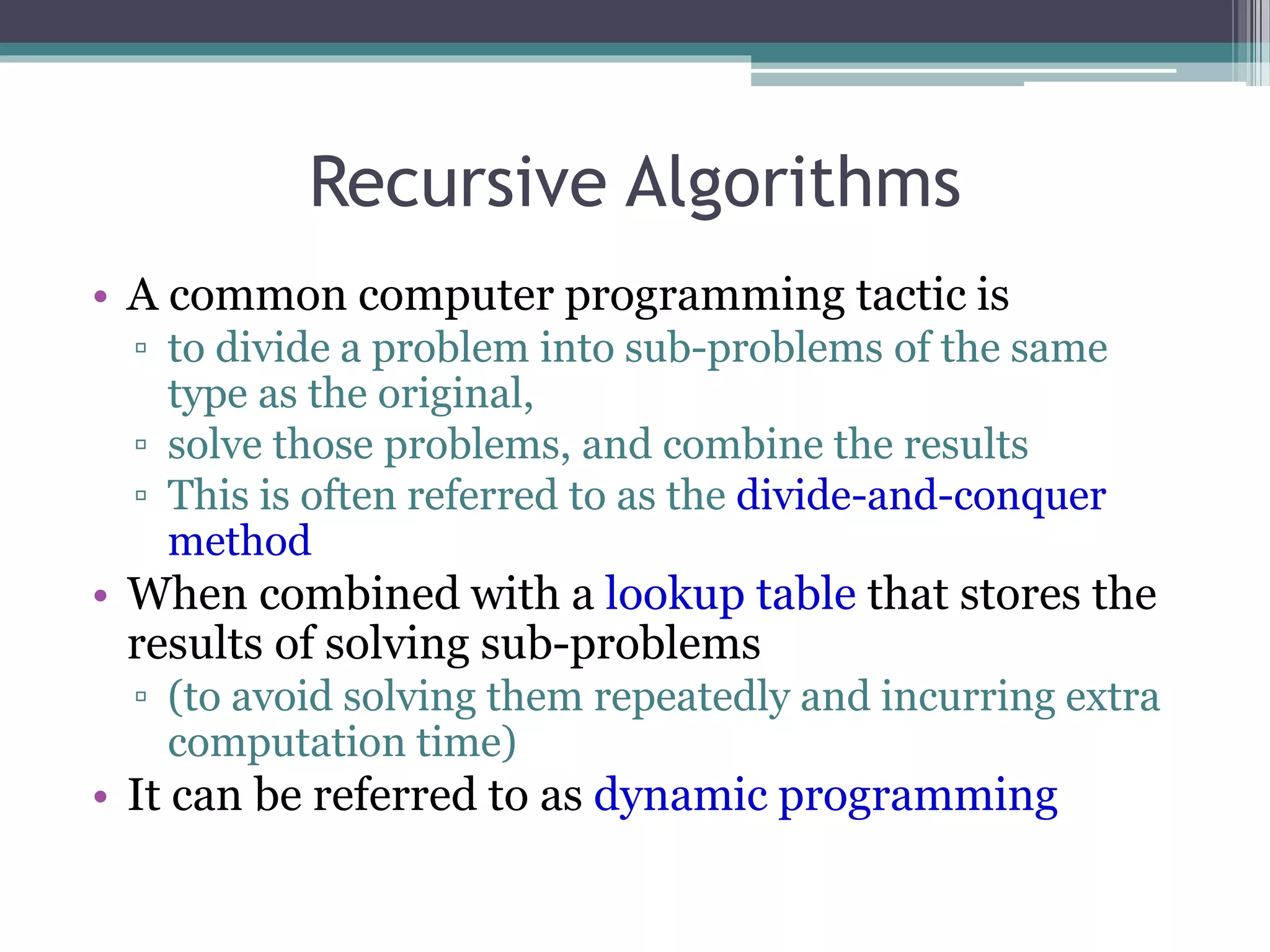
Bubble Sort Algorithm
• The Bubble Sort
algorithm looks at
pairs of entries in
the array, and swaps
their order if
needed.
[0] [1] [2] [3] [4] [5]](https://image.slidesharecdn.com/week3-recursionandsorting-191013065809/75/Recursion-and-Sorting-Algorithms-43-2048.jpg)
![0
10
20
30
40
50
60
70
[1] [2] [3] [4] [5] [6]
Bubble Sort Algorithm
• The Bubble Sort
algorithm looks at
pairs of entries in
the array, and swaps
their order if
needed.
[0] [1] [2] [3] [4] [5]
Swap?](https://image.slidesharecdn.com/week3-recursionandsorting-191013065809/75/Recursion-and-Sorting-Algorithms-44-2048.jpg)
![0
10
20
30
40
50
60
70
[1] [2] [3] [4] [5] [6]
Bubble Sort Algorithm
• The Bubble Sort
algorithm looks at
pairs of entries in
the array, and swaps
their order if
needed.
[0] [1] [2] [3] [4] [5]
Yes!](https://image.slidesharecdn.com/week3-recursionandsorting-191013065809/75/Recursion-and-Sorting-Algorithms-45-2048.jpg)
![0
10
20
30
40
50
60
70
[1] [2] [3] [4] [5] [6]
Bubble Sort Algorithm
• The Bubble Sort
algorithm looks at
pairs of entries in
the array, and swaps
their order if
needed.
[0] [1] [2] [3] [4] [5]
Swap?](https://image.slidesharecdn.com/week3-recursionandsorting-191013065809/75/Recursion-and-Sorting-Algorithms-46-2048.jpg)
![0
10
20
30
40
50
60
70
[1] [2] [3] [4] [5] [6]
Bubble Sort Algorithm
• The Bubble Sort
algorithm looks at
pairs of entries in
the array, and swaps
their order if
needed.
[0] [1] [2] [3] [4] [5]
No.](https://image.slidesharecdn.com/week3-recursionandsorting-191013065809/75/Recursion-and-Sorting-Algorithms-47-2048.jpg)
![0
10
20
30
40
50
60
70
[1] [2] [3] [4] [5] [6]
Bubble Sort Algorithm
• The Bubble Sort
algorithm looks at
pairs of entries in
the array, and swaps
their order if
needed.
[0] [1] [2] [3] [4] [5]
Swap?](https://image.slidesharecdn.com/week3-recursionandsorting-191013065809/75/Recursion-and-Sorting-Algorithms-48-2048.jpg)
![0
10
20
30
40
50
60
70
[1] [2] [3] [4] [5] [6]
Bubble Sort Algorithm
• The Bubble Sort
algorithm looks at
pairs of entries in
the array, and swaps
their order if
needed.
[0] [1] [2] [3] [4] [5]
No.](https://image.slidesharecdn.com/week3-recursionandsorting-191013065809/75/Recursion-and-Sorting-Algorithms-49-2048.jpg)
![0
10
20
30
40
50
60
70
[1] [2] [3] [4] [5] [6]
Bubble Sort Algorithm
• The Bubble Sort
algorithm looks at
pairs of entries in
the array, and swaps
their order if
needed.
[0] [1] [2] [3] [4] [5]
Swap?](https://image.slidesharecdn.com/week3-recursionandsorting-191013065809/75/Recursion-and-Sorting-Algorithms-50-2048.jpg)
![0
10
20
30
40
50
60
70
[1] [2] [3] [4] [5] [6]
Bubble Sort Algorithm
• The Bubble Sort
algorithm looks at
pairs of entries in
the array, and swaps
their order if
needed.
[0] [1] [2] [3] [4] [5]
Yes!](https://image.slidesharecdn.com/week3-recursionandsorting-191013065809/75/Recursion-and-Sorting-Algorithms-51-2048.jpg)
![0
10
20
30
40
50
60
70
[1] [2] [3] [4] [5] [6]
Bubble Sort Algorithm
• The Bubble Sort
algorithm looks at
pairs of entries in
the array, and swaps
their order if
needed.
[0] [1] [2] [3] [4] [5]
Swap?](https://image.slidesharecdn.com/week3-recursionandsorting-191013065809/75/Recursion-and-Sorting-Algorithms-52-2048.jpg)
![0
10
20
30
40
50
60
70
[1] [2] [3] [4] [5] [6]
Bubble Sort Algorithm
• The Bubble Sort
algorithm looks at
pairs of entries in
the array, and swaps
their order if
needed.
[0] [1] [2] [3] [4] [5]
Yes!](https://image.slidesharecdn.com/week3-recursionandsorting-191013065809/75/Recursion-and-Sorting-Algorithms-53-2048.jpg)
![0
10
20
30
40
50
60
70
[1] [2] [3] [4] [5] [6]
Bubble Sort Algorithm
• Repeat.
[0] [1] [2] [3] [4] [5]
Swap? No.](https://image.slidesharecdn.com/week3-recursionandsorting-191013065809/75/Recursion-and-Sorting-Algorithms-54-2048.jpg)
![0
10
20
30
40
50
60
70
[1] [2] [3] [4] [5] [6]
Bubble Sort Algorithm
• Repeat.
[0] [1] [2] [3] [4] [5]
Swap? No.](https://image.slidesharecdn.com/week3-recursionandsorting-191013065809/75/Recursion-and-Sorting-Algorithms-55-2048.jpg)
![0
10
20
30
40
50
60
70
[1] [2] [3] [4] [5] [6]
Bubble Sort Algorithm
• Repeat.
[0] [1] [2] [3] [4] [5]
Swap? Yes.](https://image.slidesharecdn.com/week3-recursionandsorting-191013065809/75/Recursion-and-Sorting-Algorithms-56-2048.jpg)
![0
10
20
30
40
50
60
70
[1] [2] [3] [4] [5] [6]
Bubble Sort Algorithm
• Repeat.
[0] [1] [2] [3] [4] [5]
Swap? Yes.](https://image.slidesharecdn.com/week3-recursionandsorting-191013065809/75/Recursion-and-Sorting-Algorithms-57-2048.jpg)
![0
10
20
30
40
50
60
70
[1] [2] [3] [4] [5] [6]
Bubble Sort Algorithm
• Repeat.
[0] [1] [2] [3] [4] [5]
Swap? Yes.](https://image.slidesharecdn.com/week3-recursionandsorting-191013065809/75/Recursion-and-Sorting-Algorithms-58-2048.jpg)
![0
10
20
30
40
50
60
70
[1] [2] [3] [4] [5] [6]
Bubble Sort Algorithm
• Repeat.
[0] [1] [2] [3] [4] [5]
Swap? Yes.](https://image.slidesharecdn.com/week3-recursionandsorting-191013065809/75/Recursion-and-Sorting-Algorithms-59-2048.jpg)
![0
10
20
30
40
50
60
70
[1] [2] [3] [4] [5] [6]
Bubble Sort Algorithm
• Loop over array n-1
times, swapping
pairs of entries as
needed.
[0] [1] [2] [3] [4] [5]
Swap? No.](https://image.slidesharecdn.com/week3-recursionandsorting-191013065809/75/Recursion-and-Sorting-Algorithms-60-2048.jpg)
![0
10
20
30
40
50
60
70
[1] [2] [3] [4] [5] [6]
Bubble Sort Algorithm
• Loop over array n-1
times, swapping
pairs of entries as
needed.
[0] [1] [2] [3] [4] [5]
Swap? Yes.](https://image.slidesharecdn.com/week3-recursionandsorting-191013065809/75/Recursion-and-Sorting-Algorithms-61-2048.jpg)
![0
10
20
30
40
50
60
70
[1] [2] [3] [4] [5] [6]
Bubble Sort Algorithm
• Loop over array n-1
times, swapping
pairs of entries as
needed.
[0] [1] [2] [3] [4] [5]
Swap? Yes.](https://image.slidesharecdn.com/week3-recursionandsorting-191013065809/75/Recursion-and-Sorting-Algorithms-62-2048.jpg)
![0
10
20
30
40
50
60
70
[1] [2] [3] [4] [5] [6]
Bubble Sort Algorithm
• Loop over array n-1
times, swapping
pairs of entries as
needed.
[0] [1] [2] [3] [4] [5]
Swap? Yes.](https://image.slidesharecdn.com/week3-recursionandsorting-191013065809/75/Recursion-and-Sorting-Algorithms-63-2048.jpg)
![0
10
20
30
40
50
60
70
[1] [2] [3] [4] [5] [6]
Bubble Sort Algorithm
• Loop over array n-1
times, swapping
pairs of entries as
needed.
[0] [1] [2] [3] [4] [5]
Swap? Yes.](https://image.slidesharecdn.com/week3-recursionandsorting-191013065809/75/Recursion-and-Sorting-Algorithms-64-2048.jpg)
![0
10
20
30
40
50
60
70
[1] [2] [3] [4] [5] [6]
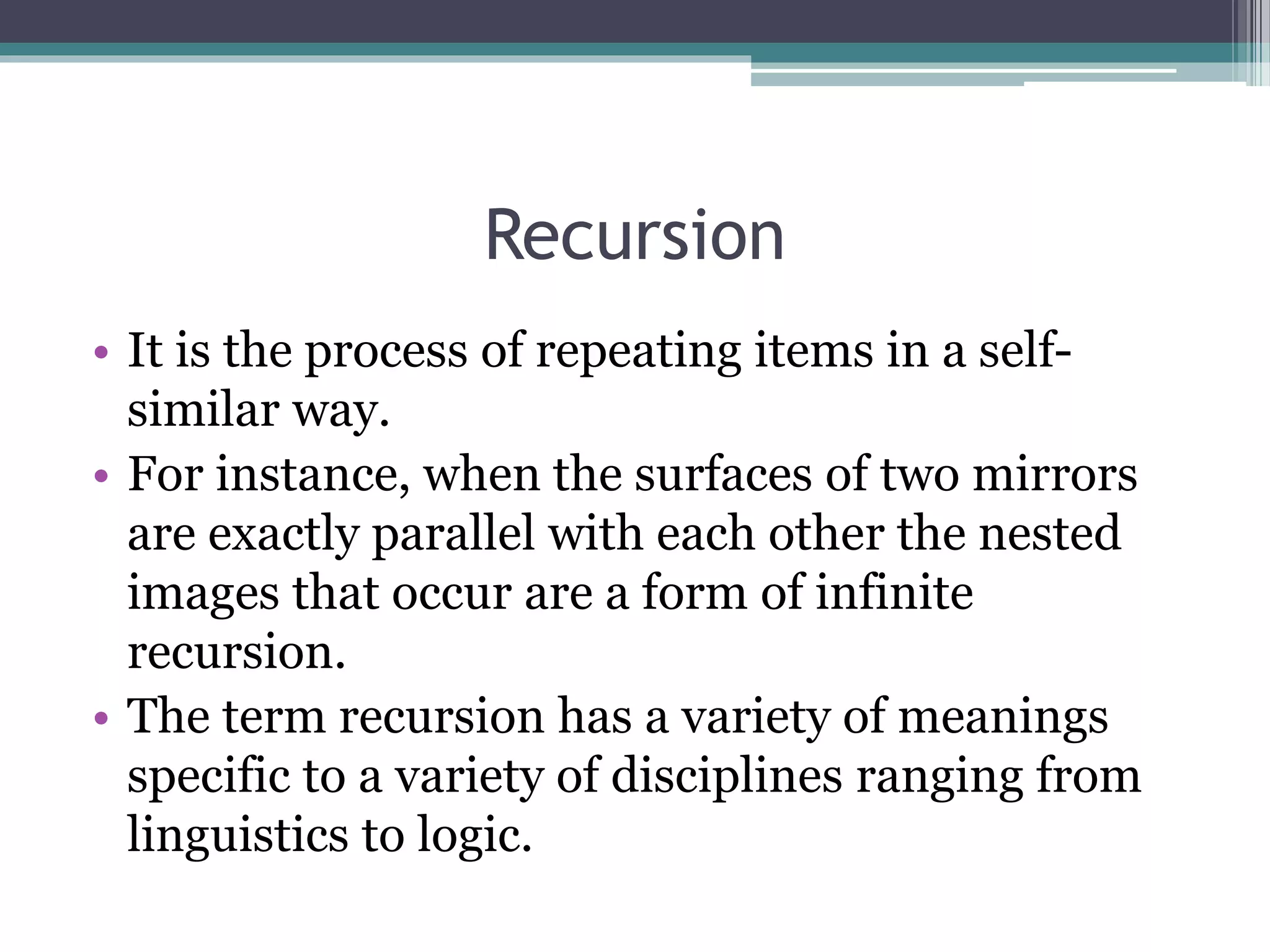
Bubble Sort Algorithm
• Continue looping,
until done.
[0] [1] [2] [3] [4] [5]
Swap? Yes.](https://image.slidesharecdn.com/week3-recursionandsorting-191013065809/75/Recursion-and-Sorting-Algorithms-65-2048.jpg)
![0
10
20
30
40
50
60
70
[1] [2] [3] [4] [5] [6]
Bubble Sort Algorithm
• Continue looping,
until done.
[0] [1] [2] [3] [4] [5]
Swap? Yes.](https://image.slidesharecdn.com/week3-recursionandsorting-191013065809/75/Recursion-and-Sorting-Algorithms-66-2048.jpg)
![0
10
20
30
40
50
60
70
[1] [2] [3] [4] [5] [6]
Bubble Sort Algorithm
• Continue looping,
until done.
[0] [1] [2] [3] [4] [5]
Swap? Yes.](https://image.slidesharecdn.com/week3-recursionandsorting-191013065809/75/Recursion-and-Sorting-Algorithms-67-2048.jpg)
![0
10
20
30
40
50
60
70
[1] [2] [3] [4] [5] [6][0] [1] [2] [3] [4] [5]
Bubble Sort Algorithm - Result](https://image.slidesharecdn.com/week3-recursionandsorting-191013065809/75/Recursion-and-Sorting-Algorithms-68-2048.jpg)
![Bubble Sort Implementation
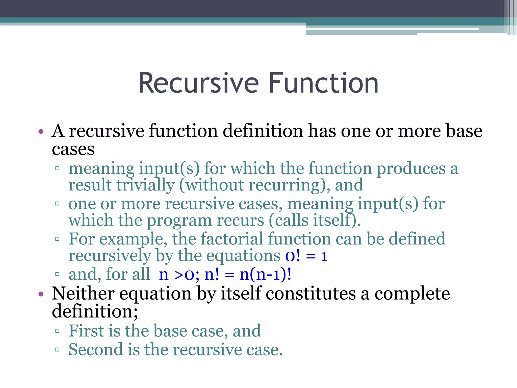
void bubbleSort (int list[ ] , int size) {
int i, j, temp;
for ( i = 0; i < size; i++ ) { /* controls passes through the list */
for ( j = 0; j < size - 1; j++ ) /* performs adjacent comparisons */
{
if ( list[ j ] > list[ j+1 ] ) /* determines if a swap should occur */
{
temp = list[ j ]; /* swap is performed */
list[ j ] = list[ j + 1 ];
list[ j+1 ] = temp;
} // end of if statement
} // end of inner for loop
} // end of outer for loop
} // end of function](https://image.slidesharecdn.com/week3-recursionandsorting-191013065809/75/Recursion-and-Sorting-Algorithms-70-2048.jpg)

The document provides an overview of recursion and sorting, detailing concepts such as recursive algorithms, algorithm analysis, linear and binary search, and various sorting methods like bubble sort. It highlights the importance of understanding recursion, its benefits and drawbacks, as well as the efficiency of different sorting techniques. The content is aimed at a foundational understanding for computer science students, illustrating practical applications and theoretical principles.
Introduction to Recursion and Sorting, search algorithms, and analysis including time complexities.
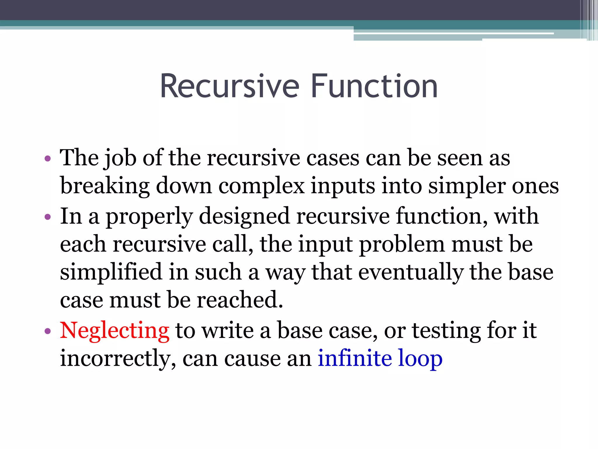
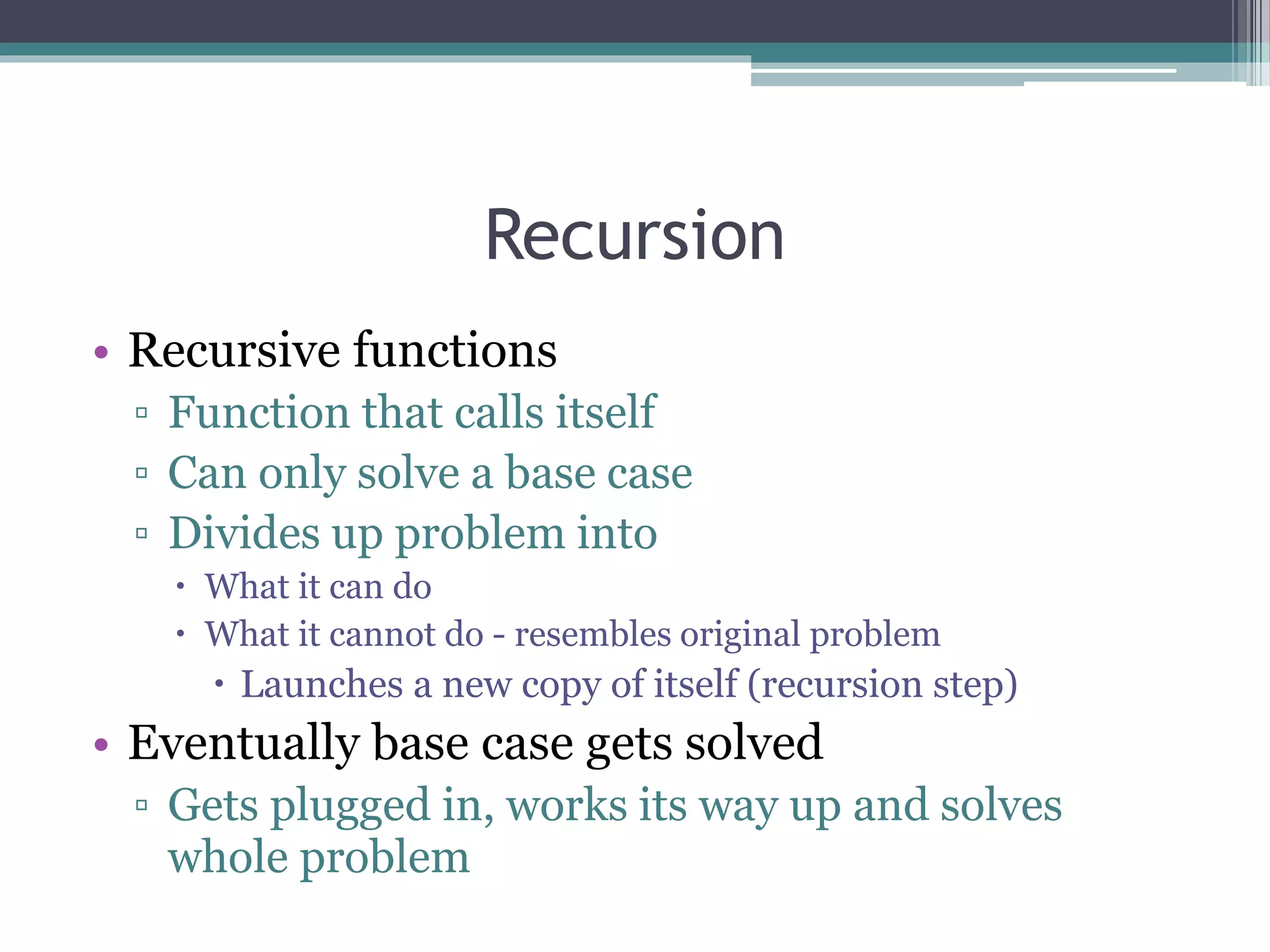
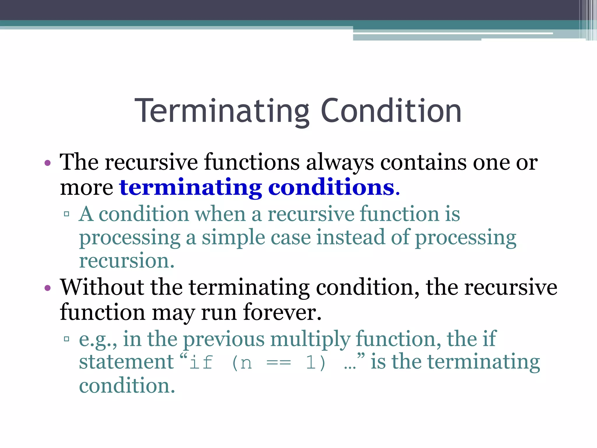
Definition of recursion with examples, recursive behavior characteristics, functions, and job breakdown.
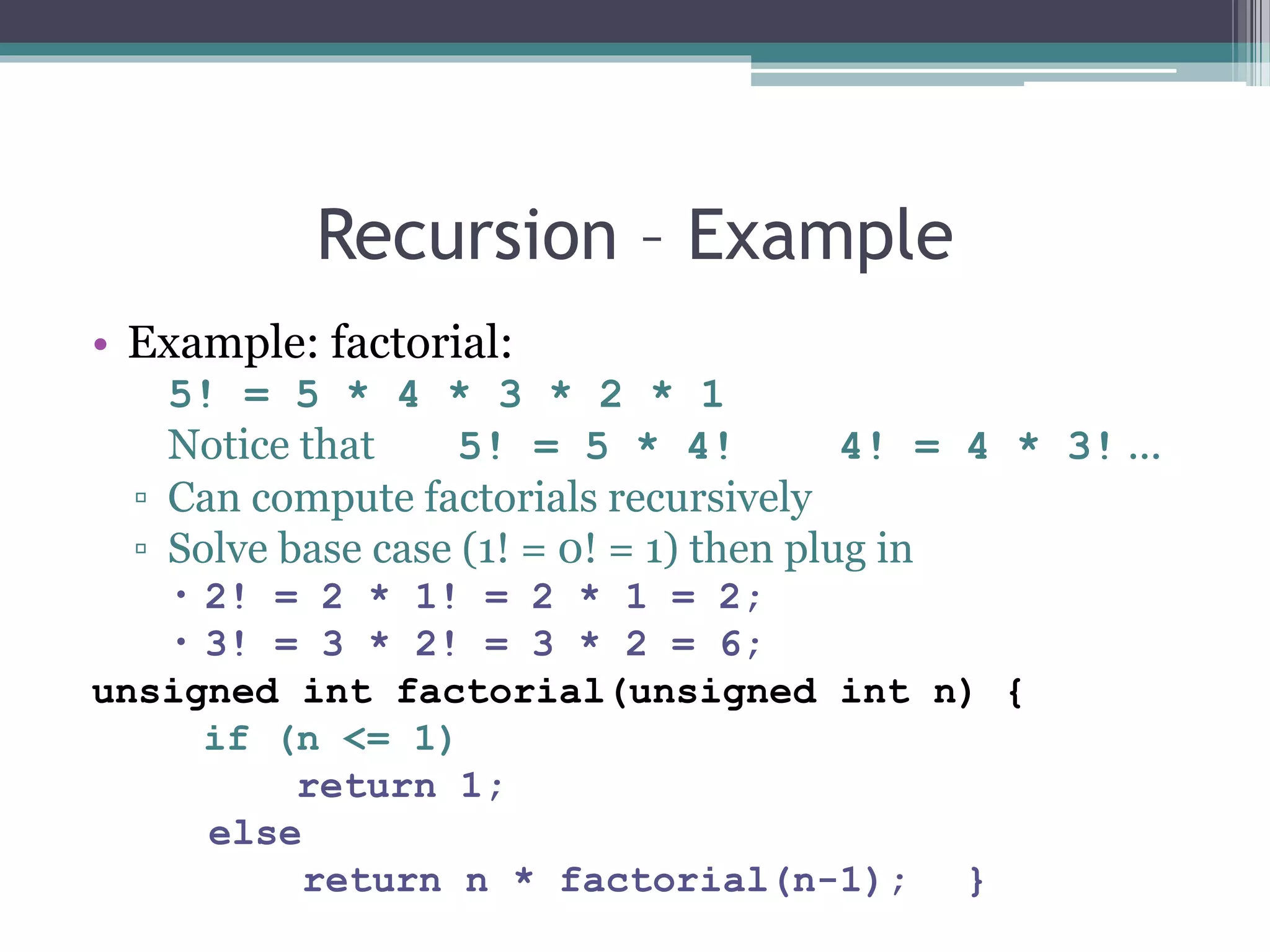
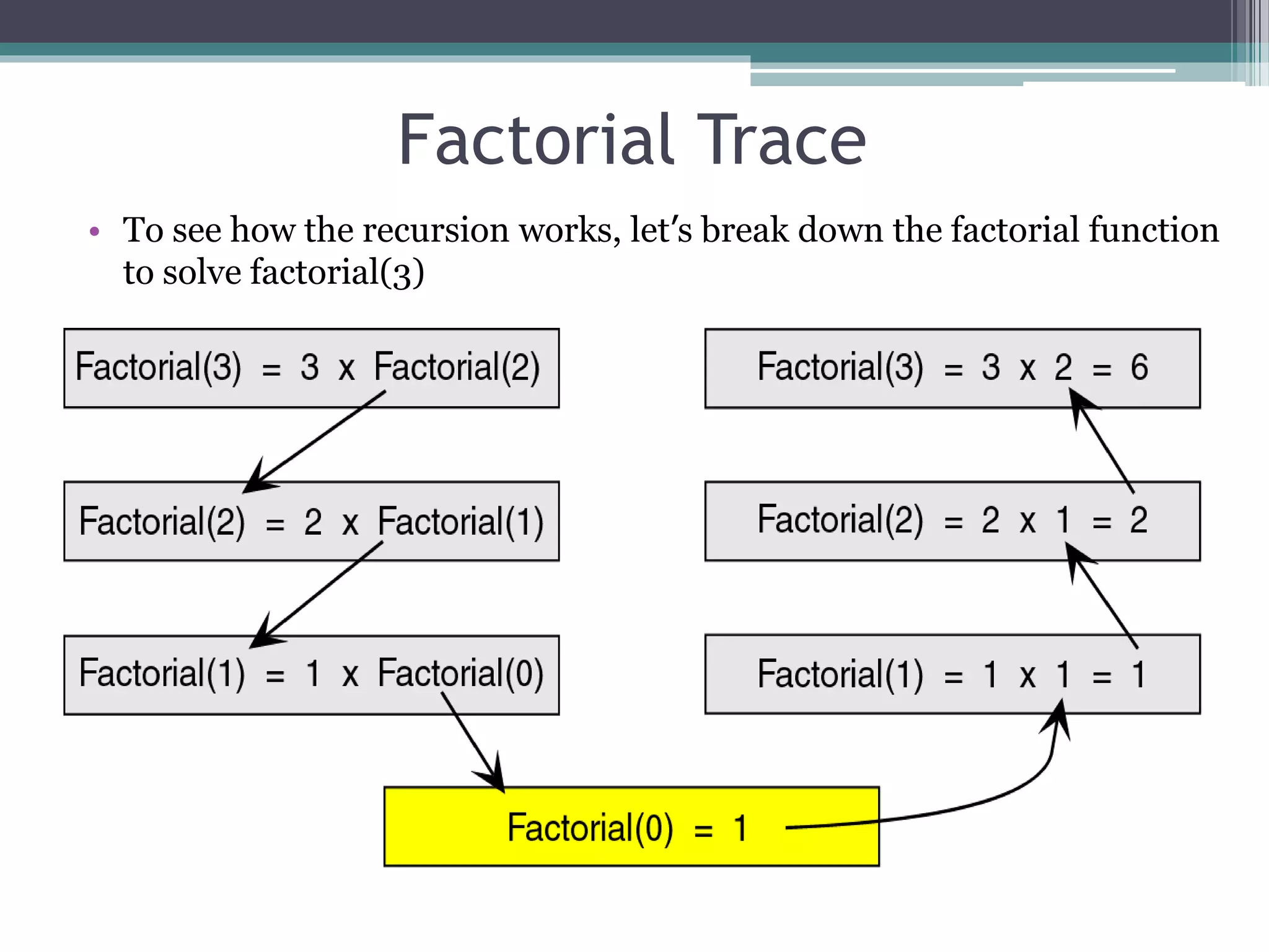
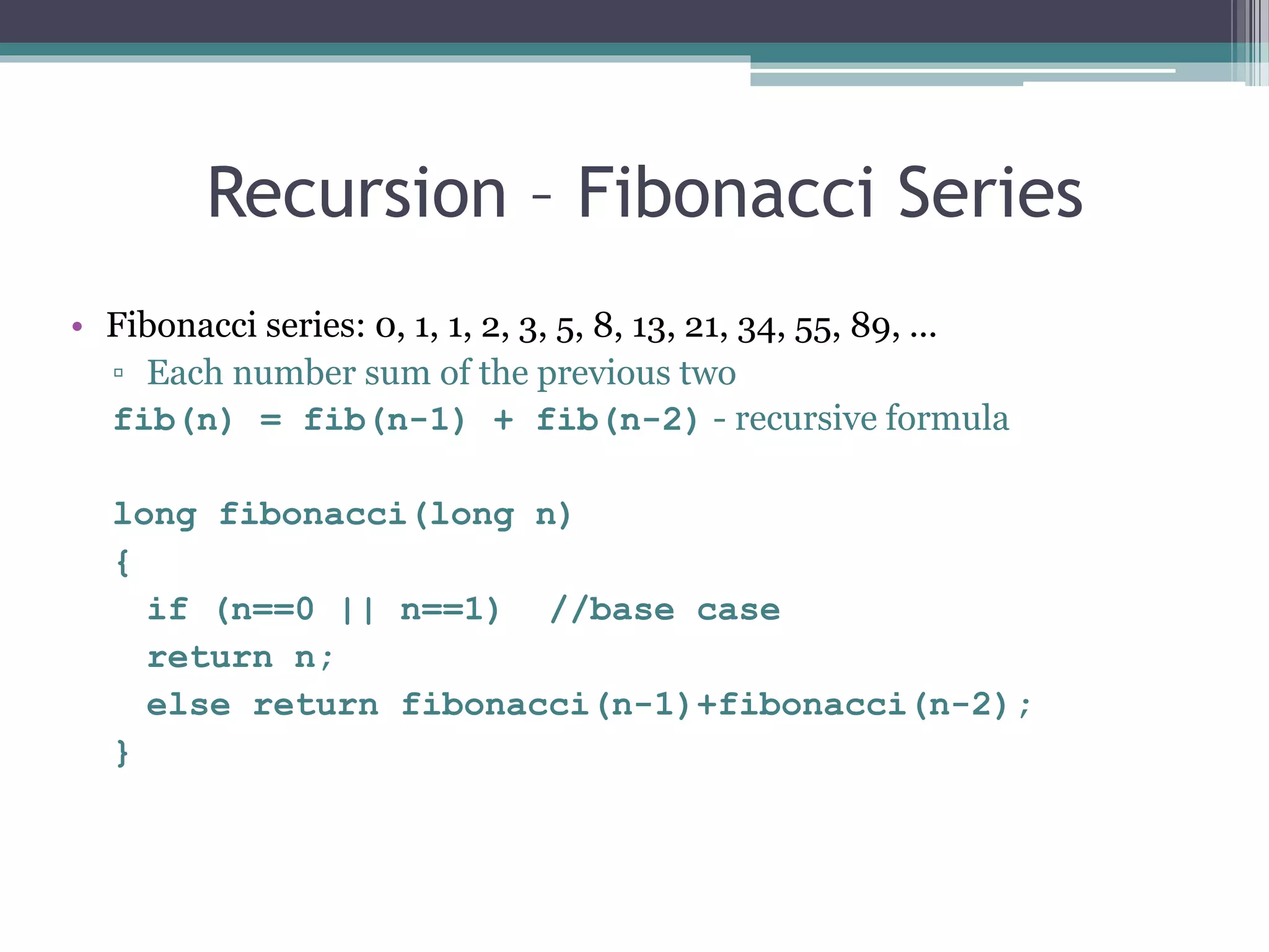
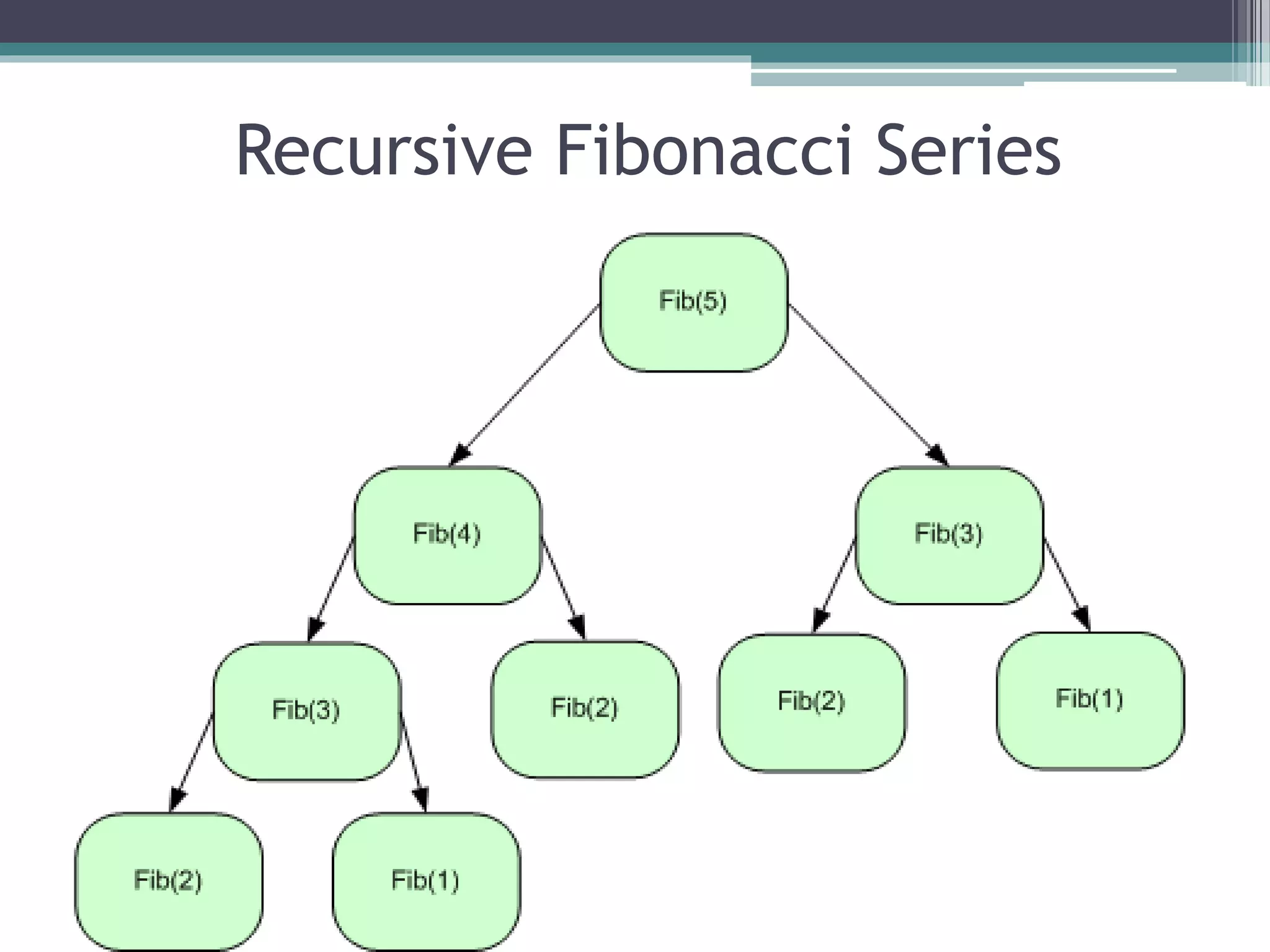
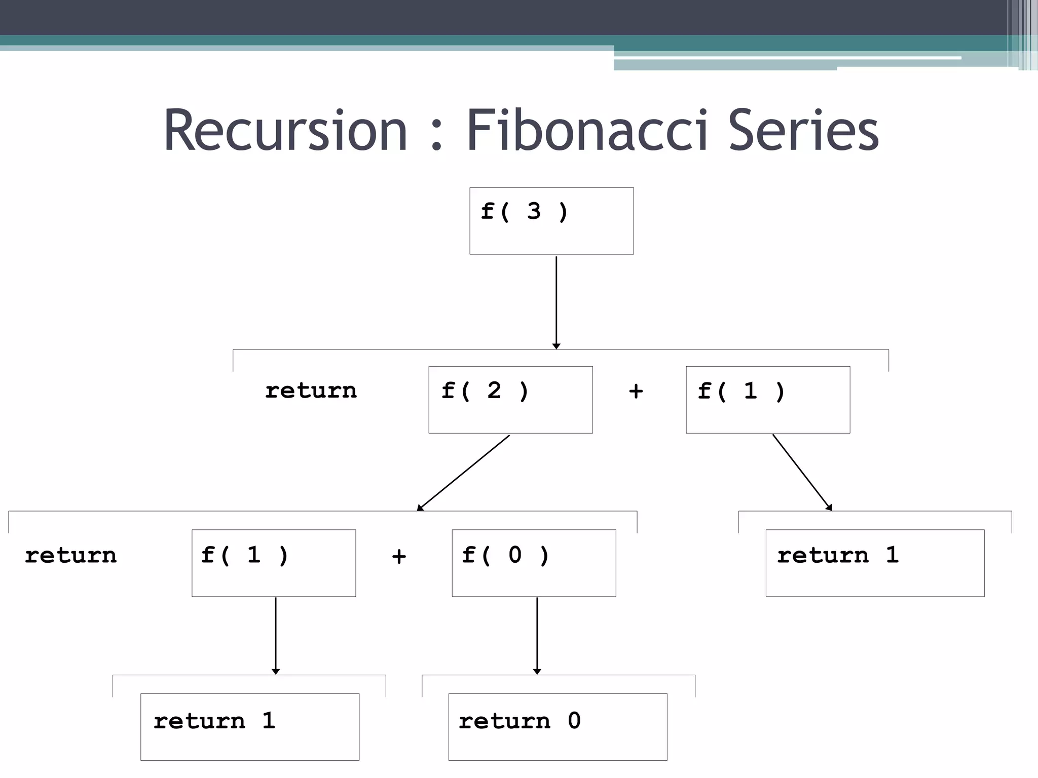
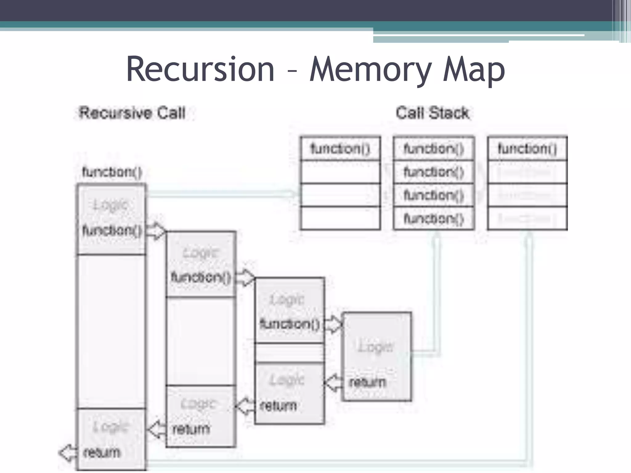
Demonstration of recursive calculation methods for factorial and Fibonacci series with memory mapping.
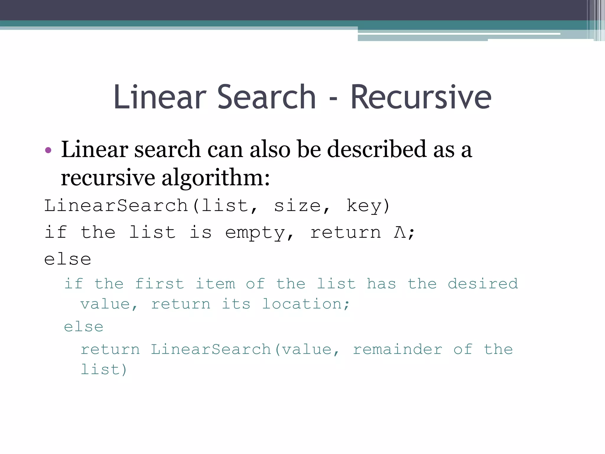
Explanation of recursive linear search and binary search implementations, showcasing algorithm differences.
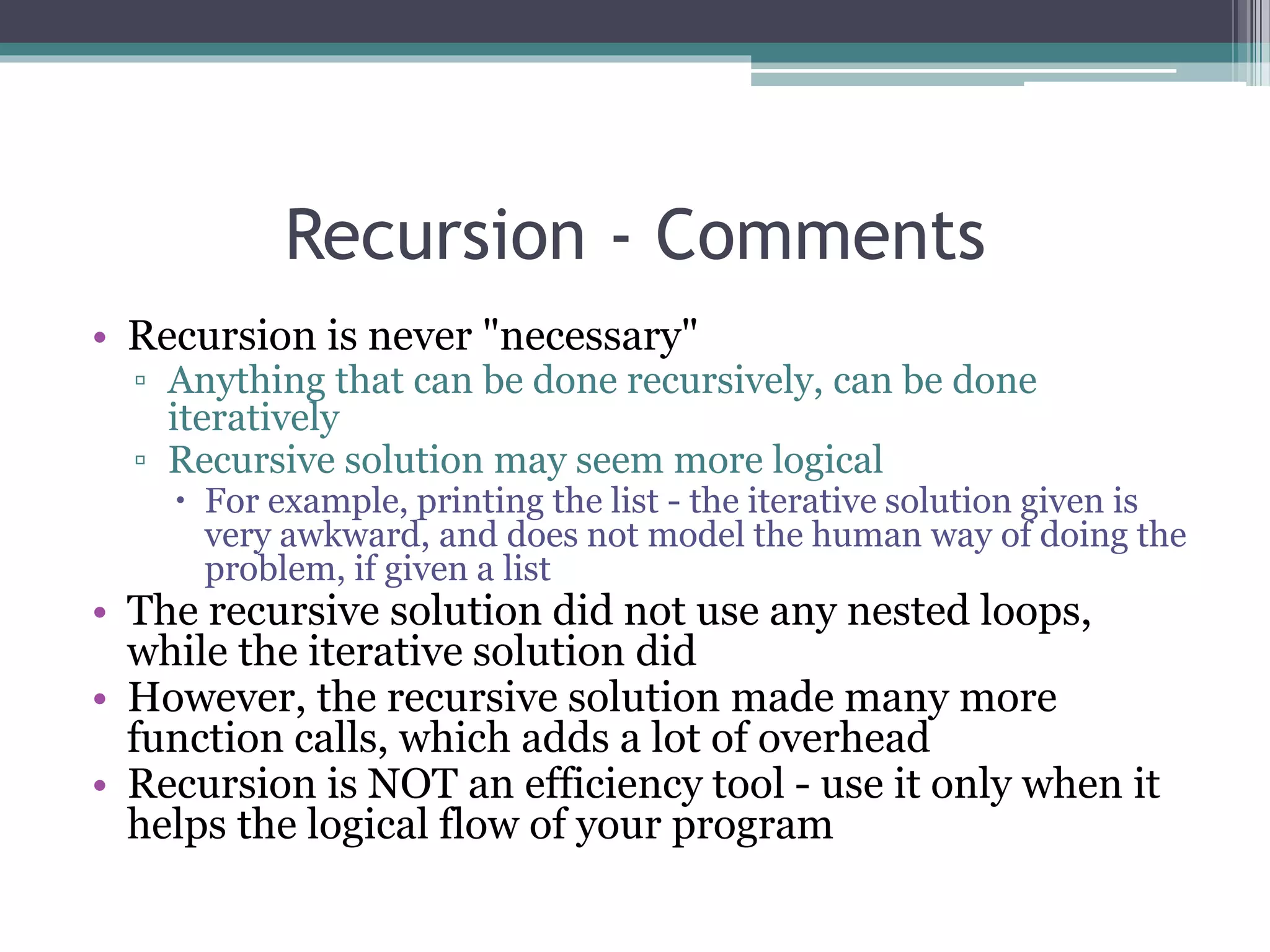
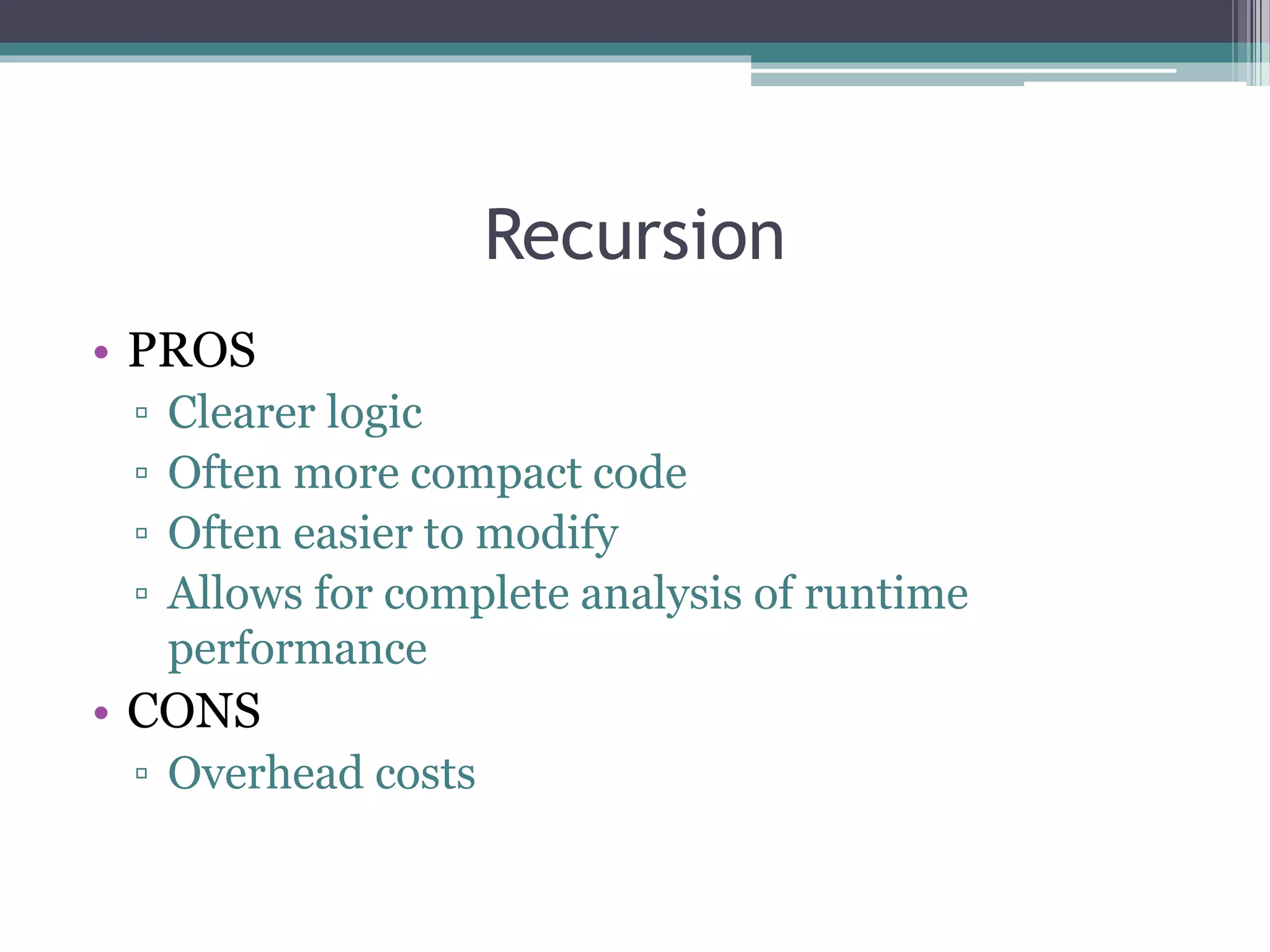
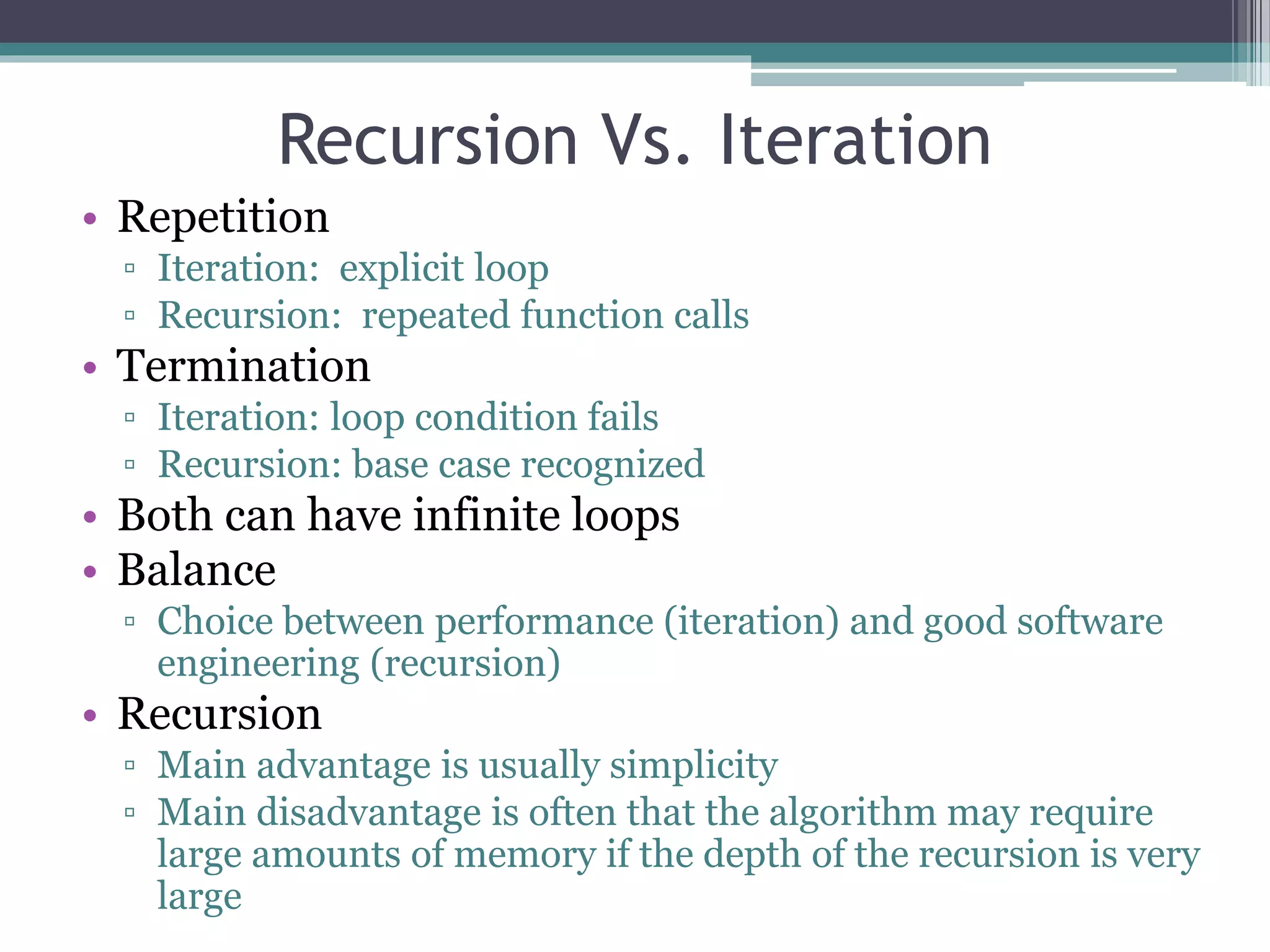
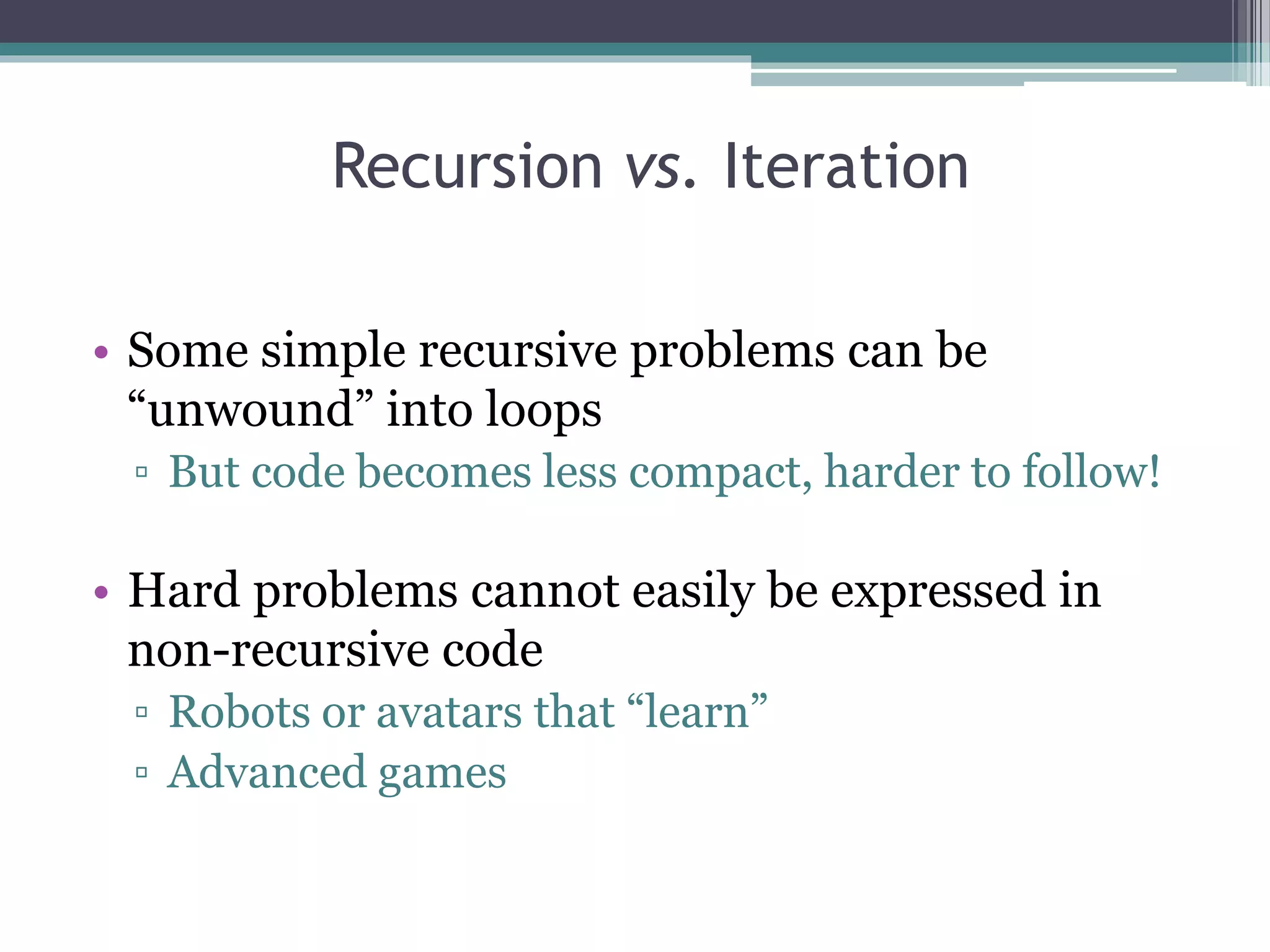
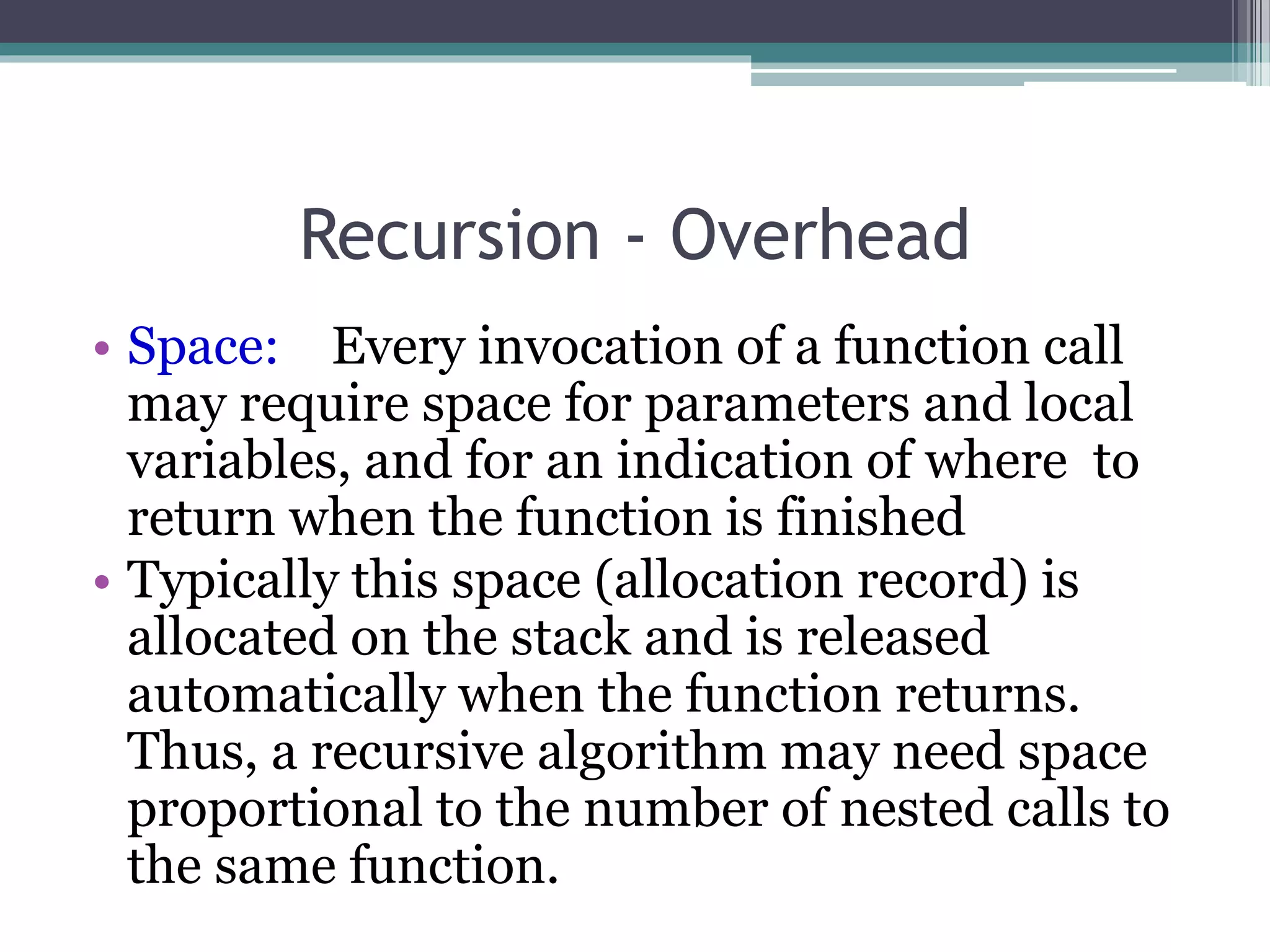
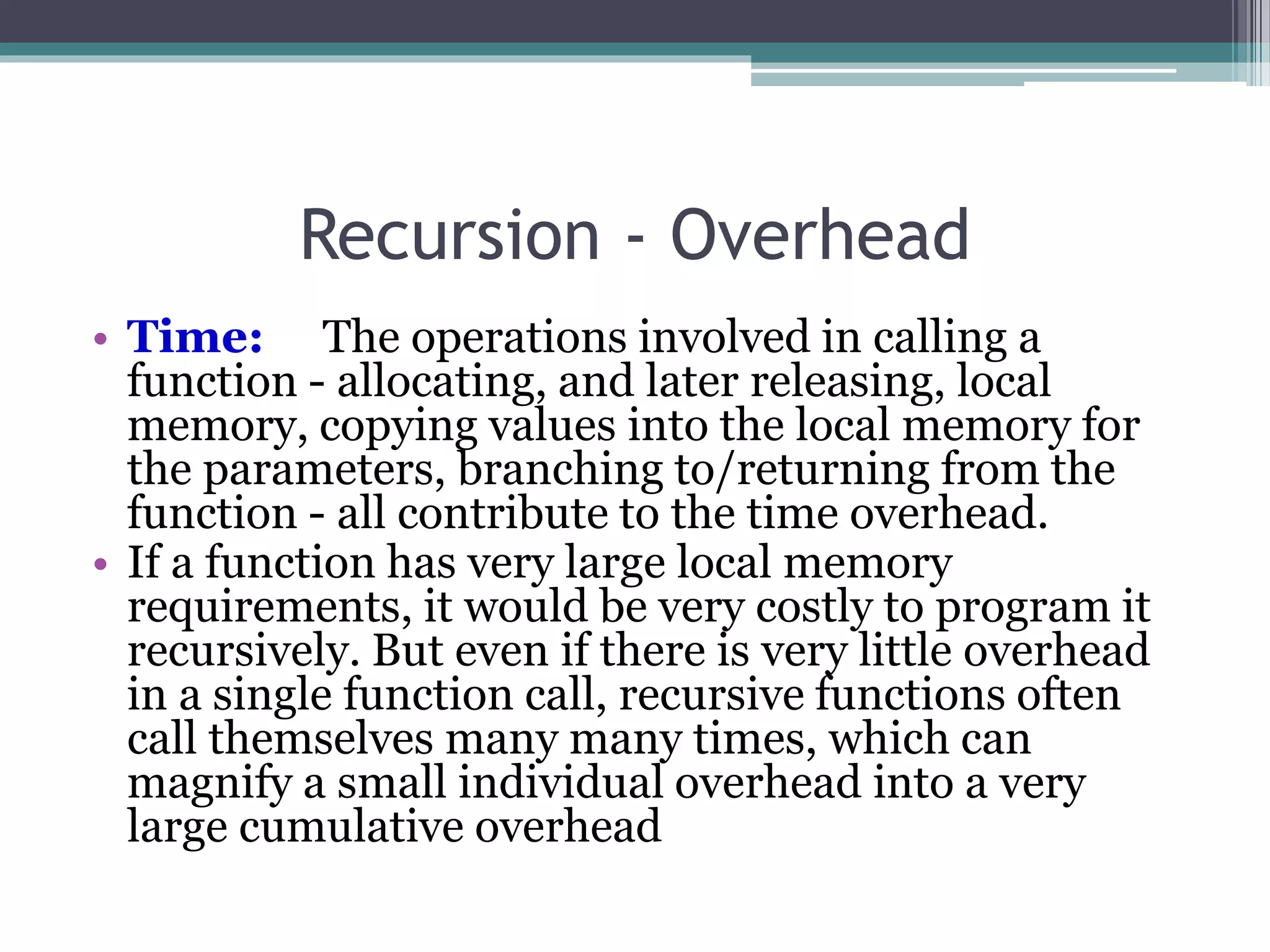
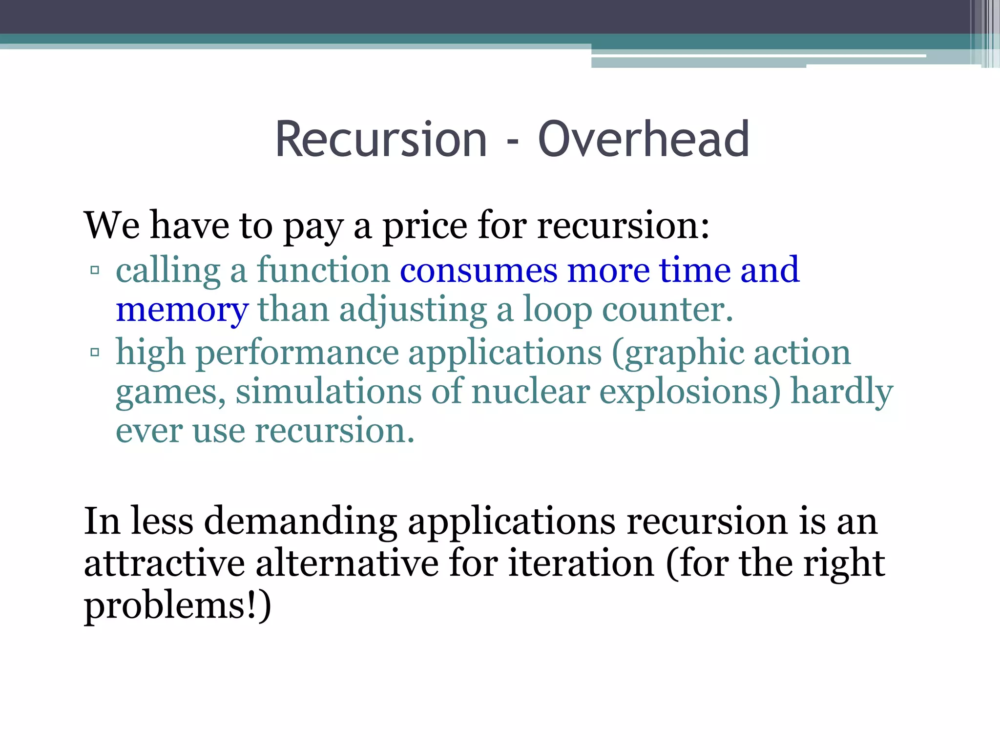
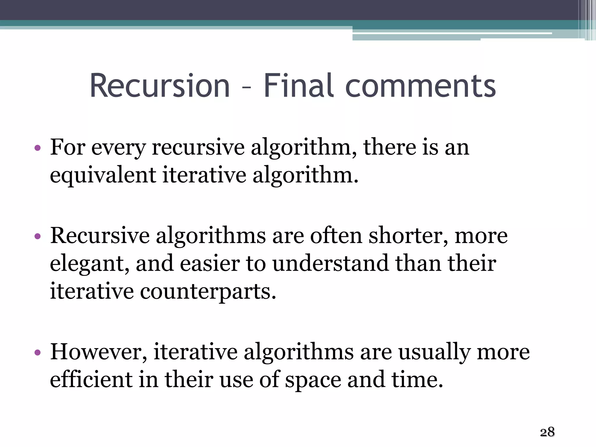
Pros and cons of recursion vs iteration, performance considerations, and memory implications in recursive functions.
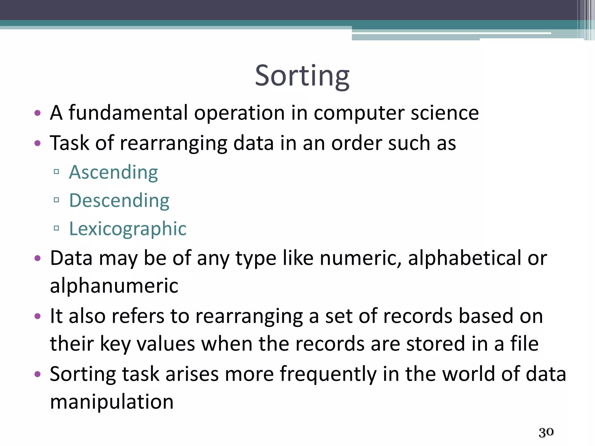
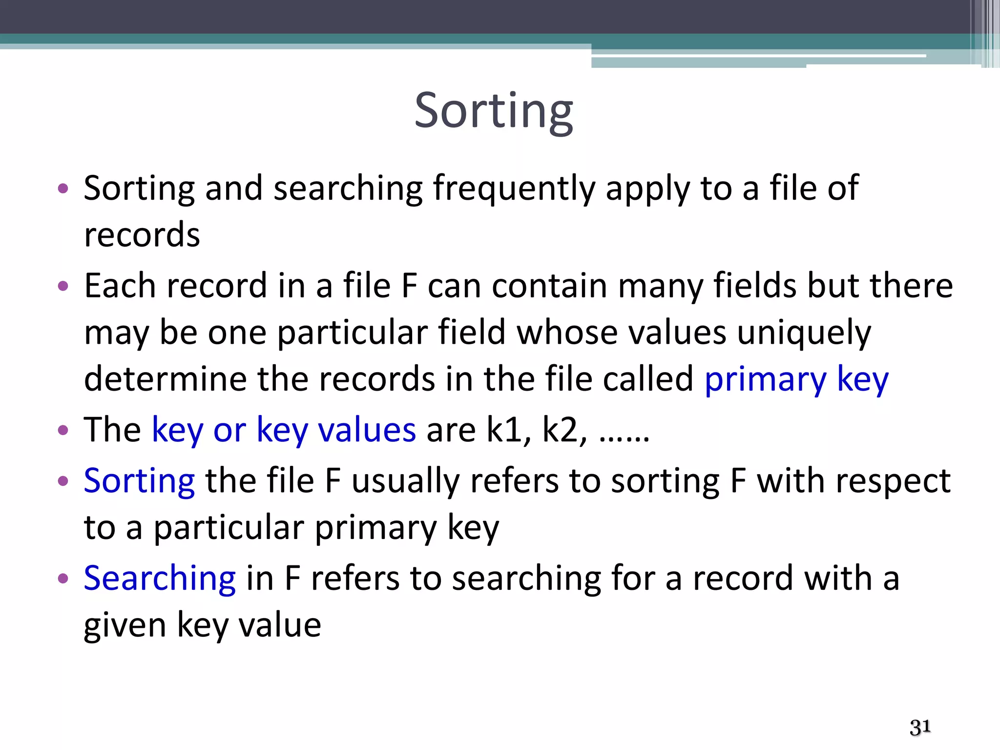
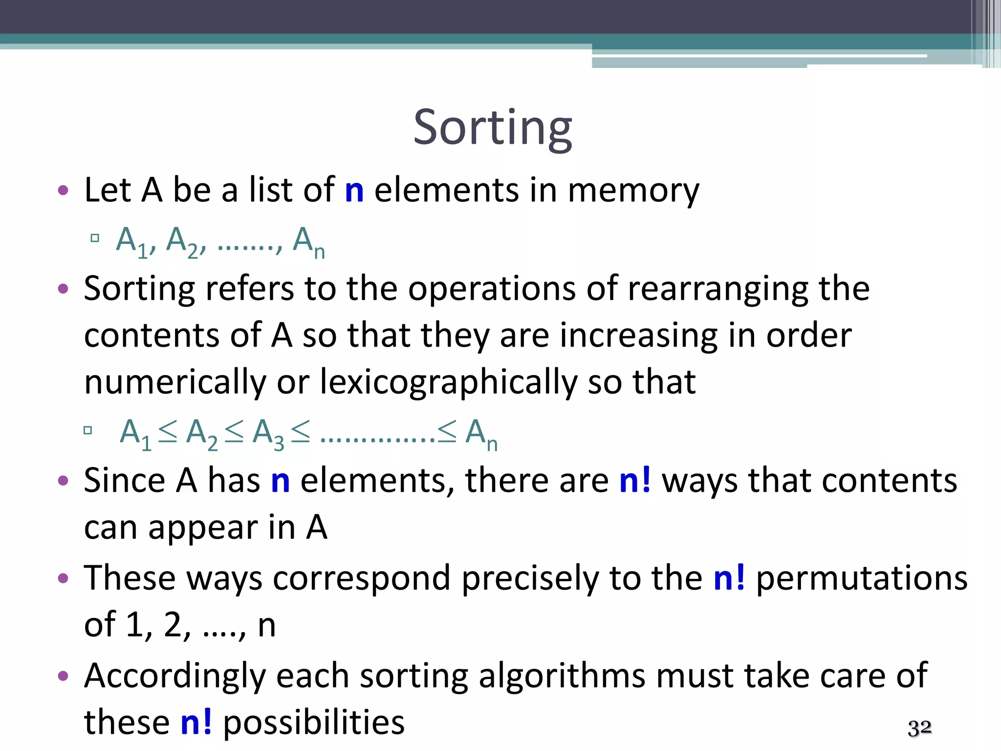
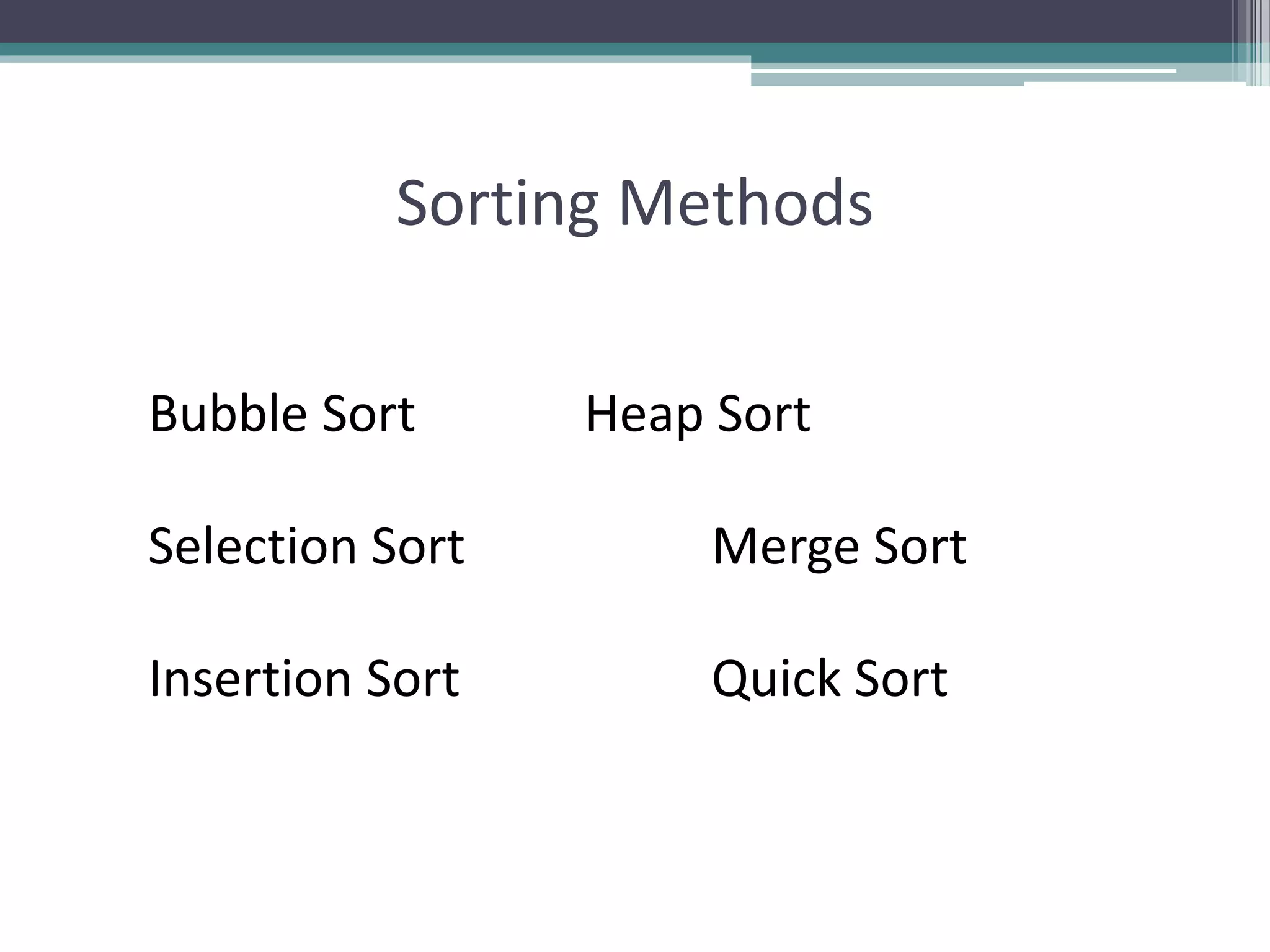
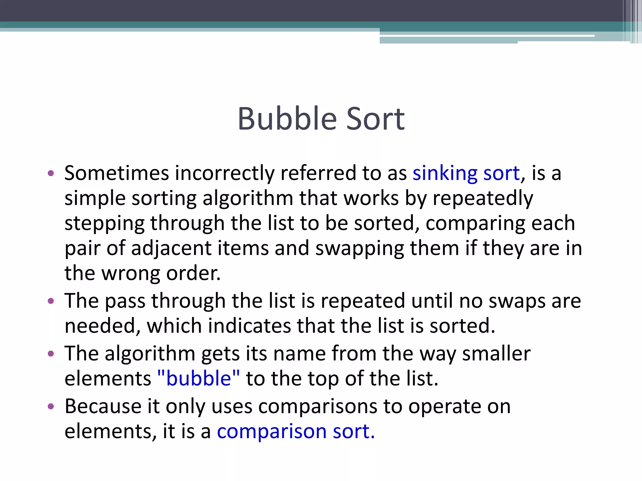
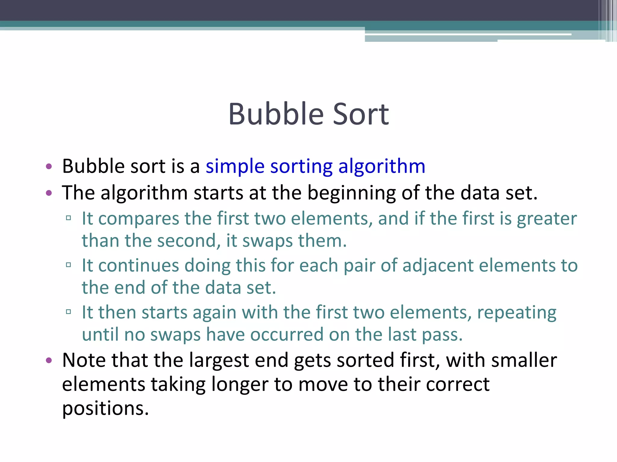
Introduction to sorting and various sorting approaches with definitions related to data arrangement.
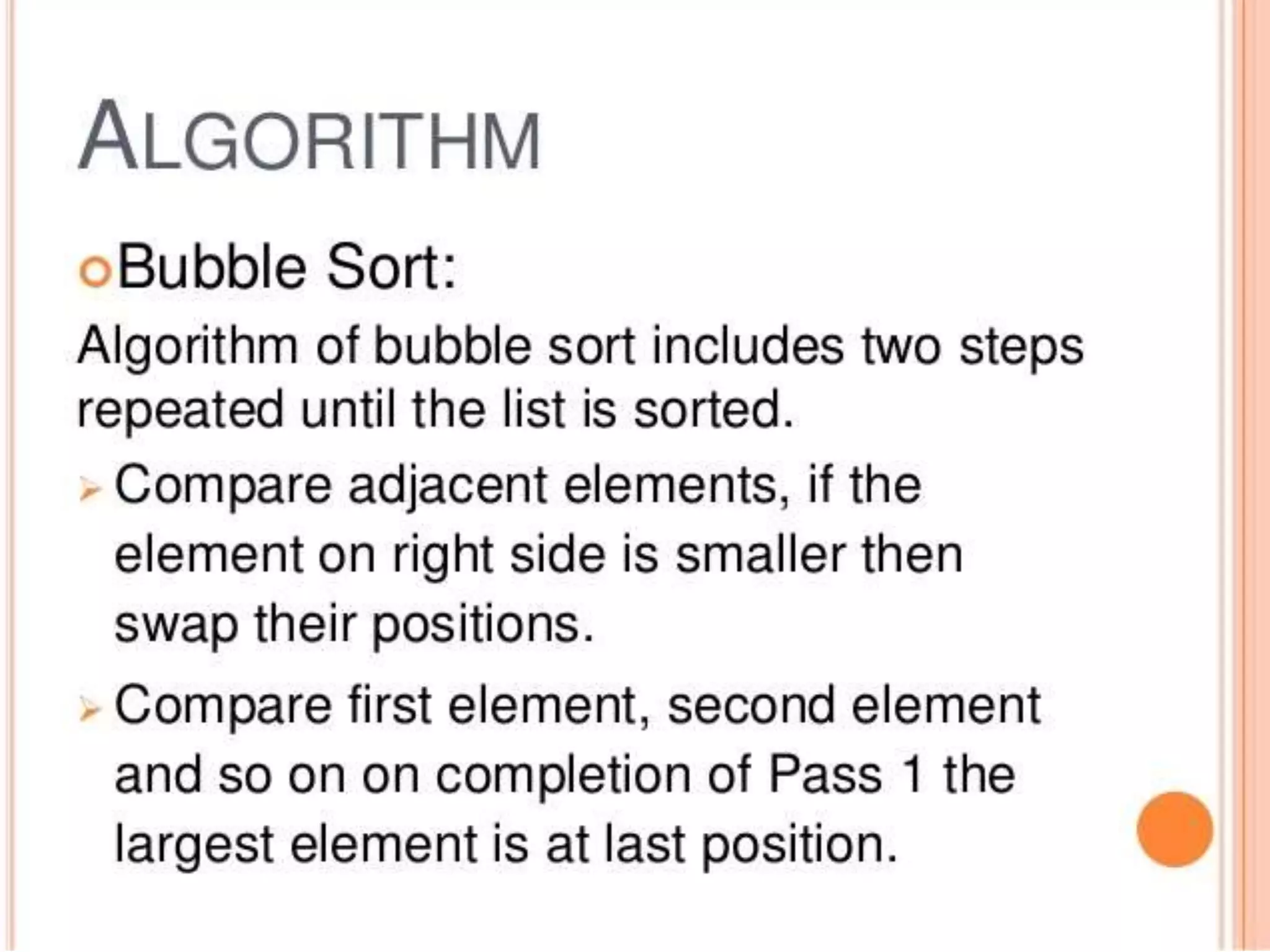
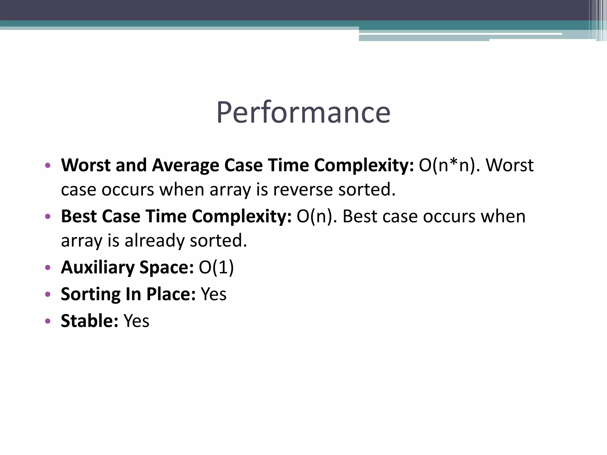
Detailed explanation of Bubble Sort algorithm with implementation, time complexity analysis, and algorithm efficiency.
List of resources for further study on recursion and sorting algorithms.