Complexity of sorting algorithms

1. Complexity of conventional Sorting
Algorithms
Course Code: CSC2211
Dept. of Computer Science
Faculty of Science and Technology
Lecturer No: Week No: 02 Semester:
Lecturer: Name & email
Course Title: Algorithms

2. Lecture Outline
1. Sorting Algorithms
 Insertion Sort
 Selection Sort
 Bubble Sort
 Merge Sort
 Quick Sort
 Counting Sort

3. Sorting
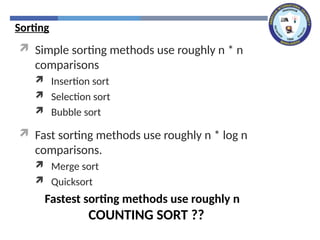
 Simple sorting methods use roughly n * n
comparisons
 Insertion sort
 Selection sort
 Bubble sort
 Fast sorting methods use roughly n * log n
comparisons.
 Merge sort
 Quicksort
COUNTING SORT ??
Fastest sorting methods use roughly n

4. Sorting Algorithms with Polynomial time

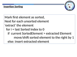
5. Insertion Sorting
Mark first element as sorted,
Next for each unsorted element
'extract' the element
for i = last Sorted Index to 0
if current SortedElement > extracted Element
move/shift sorted element to the right by 1
else: insert extracted element

6. Insertion Sorting
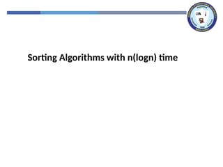
 To sort array A[0..n-1], sort A[0..n-2] recursively and
then insert A[n-1] in its proper place among the
sorted A[0..n-2]
 Usually implemented bottom up (non-recursively)
Example: 6, 4, 1, 8, 5
6 | 4 1 8 5
4 6 | 1 8 5
1 4 6 | 8 5
1 4 6 8 | 5
1 4 5 6 8

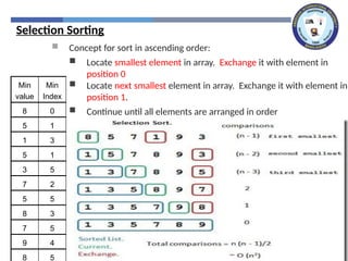
7. Selection Sorting
 Concept for sort in ascending order:
 Locate smallest element in array. Exchange it with element in
position 0
 Locate next smallest element in array. Exchange it with element in
position 1.
 Continue until all elements are arranged in order
Min
value
Min
Index
8 0
5 1
1 3
5 1
3 5
7 2
5 5
8 3
7 5
9 4
8 5

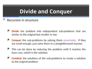
8. Selection Sort Algorithm
void selectionSort(int array[], int n)
{
int select, minIndex, minValue;
for (select = 0; select < (n - 1); select++)
{ //select the location and find the minimum value
minIndex = select;
minValue = array[select];
for(int i = select + 1; i < n; i++)
{ //start from the next of selected one to find minimum
if (array[i] < minValue)
{
minValue = array[i];
minIndex = i;
}
}
array[minIndex] = array[select];
array[select] = minValue;
}
}

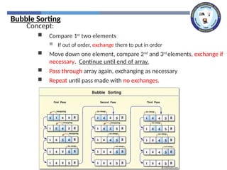
9. Bubble Sorting
Concept:
 Compare 1st
two elements
 If out of order, exchange them to put in order
 Move down one element, compare 2nd
and 3rd
elements, exchange if
necessary. Continue until end of array.
 Pass through array again, exchanging as necessary
 Repeat until pass made with no exchanges.

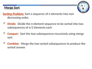
10. Bubble Sort Algorithm
void SWAP(int *a,int *b) { int t; t=*a; *a=*b;
*b=t; }
void bubble( int a[], int n ) {
int pass, j, flag;
for(pass=1;pass<n;pass++) {//break if no swap
flag = 0;
for(j=0;j<(n-pass);j++) { //discard the
last
if( a[j]>a[j+1] ) {
SWAP(&a[j+1],&a[j]); flag = 1;}
}
if (flag==0) break;
}

11. Sorting Algorithms with n(logn) time

12. Divide and Conquer
 Recursive in structure
 Divide the problem into independent sub-problems that are
similar to the original but smaller in size
 Conquer the sub-problems by solving them recursively. If they
are small enough, just solve them in a straightforward manner.
 This can be done by reducing the problem until it reaches the
base case, which is the solution.
 Combine the solutions of the sub-problems to create a solution
to the original problem

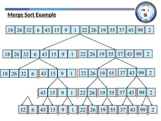
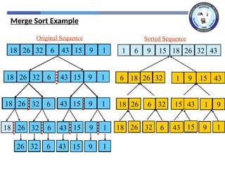
13. Merge Sort
Sorting Problem: Sort a sequence of n elements into non-
decreasing order.
 Divide: Divide the n-element sequence to be sorted into two
subsequences of n/2 elements each
 Conquer: Sort the two subsequences recursively using merge
sort.
 Combine: Merge the two sorted subsequences to produce the
sorted answer.

14. 43 15 9 1 22 26 19 55 37 43 99 2
18 26 32 6 43 15 9 1 22 26 19 55 37 43 99 2
18 26 32 6 43 15 9 1 22 26 19 55 37 43 99 2
18 26 32 6 43 15 9 1 22 26 19 55 37 43 99 2
43 15 9 1 22 26 19 55 37 43 99 2
32 6
Merge Sort Example

15. Merge Sort Example
18 26 32 6 43 15 9 1
18 26 32 6 43 15 9 1
18 26 32 6 43 15 9 1
26
18 6
32 15
43 1
9
26 32 6 43 15 9 1
18 26 32 6 43 15 9 1
18 26 32
6 15 43 1 9
6 18 26 32 1 9 15 43
1 6 9 15 18 26 32 43
26
26
18 26
32
32
6
6
32 6
18 26 32 6
43
43
15
15
43 15
9
9
1
1
9 1
43 15 9 1
18 26 32 6 43 15 9 1
18 26 6
32
6
26 32
18
15
43 1
9
1 9
15 43
1
6 9 15
18 26 32 43
Original Sequence Sorted Sequence

16. 67
45
23 14 6 33
98 42
Exercise

17. Step 1 − if it is only one element in the list it is already sorted, return.
Step 2 − divide the list recursively into two halves until it can no more be
divided. Step 3 − merge the smaller lists into new list in sorted order.
void merge_sort (int A[ ] , int start , int end )
{ if( start < end ) {
int mid = (start + end ) / 2 ;
merge_sort (A, start , mid ) ;
merge_sort (A,mid+1 , end ) ;
merge(A,start , mid , end ); }
}
void merge(int A[ ] , int start, int mid, int end) {
int i = start ,j = mid+1,i;
int B[end-start+1] , k=0;
for(z = start ;z <= end ;z++) {
if(i > mid)
B[ k++ ] = A[ j++] ;
else if ( j > end)
B[ k++ ] = A[ i++ ];
else if( A[ i ] < A[ j ])
B[ k++ ] = A[ i++ ];
else
B[ k++ ] = A[ j++];
}
for (int p=0 ; p< k ;p ++)
A[ start++ ] = B[ p ] ;
}
Merge Sort Algorithm

18. void merge_sort (int A[ ] , int start , int end )
{ if( start < end ) {
int mid = (start + end ) / 2 ;
merge_sort (A, start , mid ) ;
merge_sort (A,mid+1 , end ) ;
merge(A,start , mid , end ); }
}
void merge(int A[ ] , int start, int mid, int end) {
int i = start ,j = mid+1,i;
int B[end-start+1] , k=0;
for(z = start ;z <= end ;z++) {
if(i > mid)
B[ k++ ] = A[ j++] ;
else if ( j > end)
B[ k++ ] = A[ i++ ];
else if( A[ i ] < A[ j ])
B[ k++ ] = A[ i++ ];
else
B[ k++ ] = A[ j++];
}
for (int p=0 ; p< k ;p ++)
A[ start++ ] = B[ p ] ;

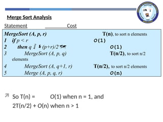
19. Statement Cost
 So T(n) = O(1) when n = 1, and
2T(n/2) + O(n) when n > 1
MergeSort (A, p, r) T(n), to sort n elements
1 if p < r O(1)
2 then q  (p+r)/2 O(1)
3 MergeSort (A, p, q) T(n/2), to sort n/2
elements
4 MergeSort (A, q+1, r) T(n/2), to sort n/2 elements
5 Merge (A, p, q, r) O(n)
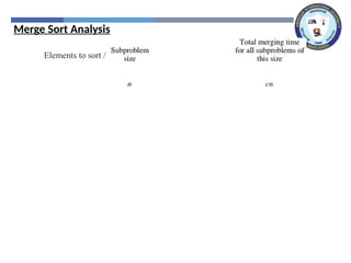
Merge Sort Analysis

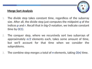
20. 1. The divide step takes constant time, regardless of the subarray
size. After all, the divide step just computes the midpoint q of the
indices p and r. Recall that in big-O notation, we indicate constant
time by O(1).
2. The conquer step, where we recursively sort two subarrays of
approximately n/2 elements each, takes some amount of time,
but we'll account for that time when we consider the
subproblems.
3. The combine step merges a total of n elements, taking O(n) time.
Merge Sort Analysis

21. Elements to sort /
Merge Sort Analysis

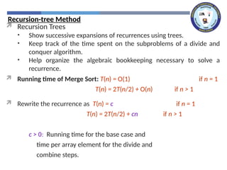
22. Recursion-tree Method
 Recursion Trees
• Show successive expansions of recurrences using trees.
• Keep track of the time spent on the subproblems of a divide and
conquer algorithm.
• Help organize the algebraic bookkeeping necessary to solve a
recurrence.
 Running time of Merge Sort: T(n) = O(1) if n = 1
T(n) = 2T(n/2) + O(n) if n > 1
 Rewrite the recurrence as T(n) = c if n = 1
T(n) = 2T(n/2) + cn if n > 1
c > 0: Running time for the base case and
time per array element for the divide and
combine steps.

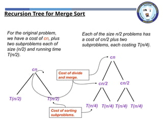
23. Recursion Tree for Merge Sort
For the original problem,
we have a cost of cn, plus
two subproblems each of
size (n/2) and running time
T(n/2).
cn
T(n/2) T(n/2)
Each of the size n/2 problems has
a cost of cn/2 plus two
subproblems, each costing T(n/4).
cn
cn/2 cn/2
T(n/4) T(n/4) T(n/4) T(n/4)
Cost of divide
and merge.
Cost of sorting
subproblems.

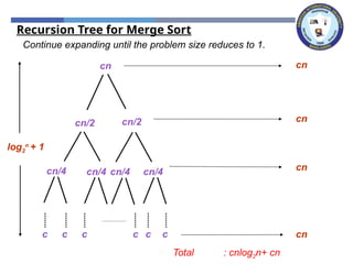
24. Continue expanding until the problem size reduces to 1.
cn
cn/2 cn/2
cn/4 cn/4 cn/4 cn/4
c c c c
c c
log2
n
+ 1
cn
cn
cn
cn
Recursion Tree for Merge Sort
Total : cnlog2n+ cn

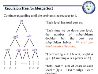
25. Continue expanding until the problem size reduces to 1.
cn
cn/2 cn/2
cn/4 cn/4 cn/4 cn/4
c c c c
c c
•Each level has total cost cn.
•Each time we go down one level,
the number of subproblems
doubles, but the cost per
subproblem halves  cost per
level remains the same.
•There are lg n + 1 levels, height is
lg n. (Assuming n is a power of 2.)
•Total cost = sum of costs at each
level = (lg n + 1)cn = cnlgn + cn =
Recursion Tree for Merge Sort

26. Analysis: solving recurrence
)
log
(
log
)
2
(
2
)
(
n
n
O
n
n
n
kn
n
T
n
T k
k





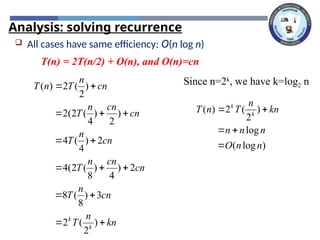
 All cases have same efficiency: O(n log n)
T(n) = 2T(n/2) + O(n), and O(n)=cn
kn
n
T
cn
n
T
cn
cn
n
T
cn
n
T
cn
cn
n
T
cn
n
T
n
T
k
k














)
2
(
2
3
)
8
(
8
2
)
4
)
8
(
2
(
4
2
)
4
(
4
)
2
)
4
(
2
(
2
)
2
(
2
)
( Since n=2k
, we have k=log2 n

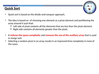
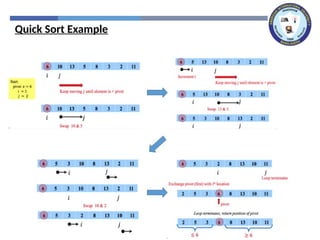
27. • Quick sort is based on the divide-and-conquer approach.
• The idea is based on of choosing one element as a pivot element and partitioning the
array around it such that:
 Left side of pivot contains all the elements that are less than the pivot element.
 Right side contains all elements greater than the pivot.
• It reduces the space complexity and removes the use of the auxiliary array that is used
in merge sort.
• Selecting a random pivot in an array results in an improved time complexity in most of
the cases.
Quick Sort

28. Quick_sort ( A[ ] , start , end ) {
if( start < end ) {
piv_pos = Partition (A,start , end ) ;
Quick_sort (A, start , piv_pos -1);
Quick_sort ( A, piv_pos +1 , end) ; } }
Partition ( A[], start , end) {
i = start + 1;
piv = A[start] ;
for( j =start + 1; j <= end ; j++ ) {
if ( A[ j ] < piv) {
swap (A[ i ],A [ j ]);
i += 1;
}
}
swap ( A[ start ] ,A[ i-1 ] ) ;
return i-1;}
Quick Sort Algorithm

29. Quick Sort Example

30. Sorting Algorithms with linear time

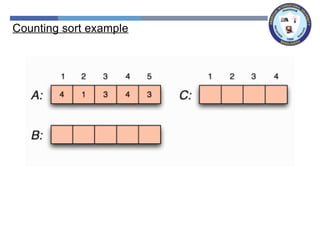
31. orti Counting sort: No comparisons between elements.
Input: A[1 . . n], where A[j] ∈ {1, 2, . . . , k}.
Output: B[1 . . n], sorted.
Auxiliary storage: C [1 . . k].
12 /
Counting Sort
do C [i ] ←
0
do C [A[j]] ← C [A[j]] +
1
do C [i ] ← C [i ] + C [i
− 1]
d C [i ] = |{key =
i }|
d C [i ] = |{key ≤ i
}|
do B[C [A[j]]] ←
A[j]
1 for i ← 1 to k
2
3 for j ← 1 to n
4
5 for i ← 2 to k
6
7 for j ← n downto 1
8
9 C [A[j]] ← C [A[j]] −
1

32. Counting sort example

33. Counting sort example Loop 1
for i ←1 to k
do C [i ] ←0

34. Counting sort example Loop 2
for j ←1 to n
do C [A[j ]] ←C [A[j ]] + 1 C [i ] = |{key = i}|

35. Counting sort example Loop 2
for j ←1 to n
do C [A[j ]] ←C [A[j ]] + 1 C [i ] = |{key = i}|

36. Counting sort example Loop 2
for j ←1 to n
do C [A[j ]] ←C [A[j ]] + 1 C [i ] = |{key = i}|

37. Counting sort example Loop 2
for j ←1 to n
do C [A[j ]] ←C [A[j ]] + 1 C [i ] = |{key = i}|

38. Counting sort example Loop 2
for j ←1 to n
do C [A[j ]] ←C [A[j ]] + 1 C [i ] = |{key = i}|

39. Counting sort example Loop 3
for i ←2 to k
do C [i ] ←C [i ] + C [i −1] C [i ] = |{key ≤i}|

40. Counting sort example Loop 3
for i ←2 to k
do C [i ] ←C [i ] + C [i −1] C [i ] = |{key ≤i}|

41. Counting sort example Loop 3
for i ←2 to k
do C [i ] ←C [i ] + C [i −1] C [i ] = |{key ≤i}|

42. Counting sort example loop 4
for j ←n downto 1
do B[C [A[j ]]] ←A[j ]
C [A[j ]] ←C [A[j ]] −1

43. Counting sort example Loop 4
for j ←n downto 1
do B[C [A[j ]]] ←A[j ]
C [A[j ]] ←C [A[j ]] −1

44. Counting sort example Loop 4
for j ←n downto 1
do B[C [A[j ]]] ←A[j ]
C [A[j ]] ←C [A[j ]] −1

45. Counting sort example Loop 4
for j ←n downto 1
do B[C [A[j ]]] ←A[j ]
C [A[j ]] ←C [A[j ]] −1

46. Counting sort example Loop 4
for j ←n downto 1
do B[C [A[j ]]] ←A[j ]
C [A[j ]] ←C [A[j ]] −1

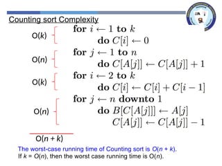
47. O(k)
O(n)
O(k)
O(n)
O(n + k)
Counting sort Complexity
The worst-case running time of Counting sort is O(n + k).
If k = O(n), then the worst case running time is O(n).

48. Books
Introduction to Algorithms, Thomas H. Cormen, Charle E. Leiserson,
Ronald L. Rivest, Clifford Stein (CLRS).
Fundamental of Computer Algorithms, Ellis Horowitz, Sartaj Sahni, Sanguthevar Rajasekaran (HSR)

49. References
https://www.google.com/search?q=bubble+sort+
step+by+step&sxsrf=ALeKk01uxzgfT3Oy6k1Q3WxVnSpiIN8_4g:1587999728942
&tbm=isch&source=iu&ictx=1&fir=vRwFsGwVfJ6pJM%253A%252CSzhhze6MPQr4c
M%252C_&vet=1&usg=AI4_-kSrEEXqwRL-PkHhVUtn7jNfF9dB6g&sa=X&ved=2ahUK
Ewje0Pz974jpAhXRAnIKHWhMD2UQ_h0wAXoECAcQBg#imgrc=EN4Sdu7veOWVo
M&imgdii=eOqvCu85p9-eBM
https://www.interviewcake.com/concept/java/counting-sort
https://www.geeksforgeeks.org/counting-sort/
https://www.hackerearth.com/practice/algorithms/sorting/quick-sort/tutorial/