1. Jigar Patel (jbpatel4@Illinois.edu), Advisor: Dr. Richard Sowers
Department of Industrial and Enterprise Systems Engineering, College of Engineering, University of Illinois at Urbana-Champaign
Modelling Basic Financial Cycles of Businesses Using Physical Mass-Spring System
8. Acknowledgments
I am grateful to Dr. Richard Sowers in the ISE department
for his guidance through this project. A special mention
goes to Sir Peter Itskovich for his assistant with editing the
computer code.
7. Future Improvements
The current model is a very rough parallel to realistic
economic cycles. Below is a small list which can help in a
more accurate depiction of the dynamic economic cycle:
1. Redefining the parallels between physical and economic
variables to reduce error.
• Use Profitability Ratios
2. Construct different models for different industries.
3. Incorporate additional factors besides stock prices as
external forces affecting the system.
4. Improve computer code to display and change critical
parameters such as oscillation frequency.
5. Build in predictive power to help businesses forecast
their financial future.
2. Background
The displacement of a physical mass-spring system, subject
to a forced oscillator, as represented by a Fourier Series,
is given by:
1. Introduction
Many phenomena follow some sort of oscillation. The
intriguing part about cycles is that it enables us to make
predictions. One must know some basic parameters which
govern the oscillation, and then, one can test the effects of
tweaking a variable to see how the oscillation changes. So
theoretically, we can fine tune all of the variables to get the
desired oscillation.
This research focuses on the physical mass-spring
system and uses the mathematical models describing the
motion of the mass to describe the economic fluctuations in
a business’s finance. The crux of the research is to first
translate the physical variables into economic variables and
then enter them in the mathematical model to replicate or
forecast the financial figures for a business.
4. Method
The economic model relies on the mathematical models
used to describe a physical mass-spring system.
1. Variable Translation: The mass-spring system equations
are written in terms of physical variables, so we first
translate or parallel physical variables with basic
financial variables.
2. Data Acquisition: The economic model requires financial
data, so we obtain the Income Statement, historical stock
prices, and the average enterprise value from any
finance website.
3. Implementation: The mathematical models describing
the physical oscillations are now applied to the
economic variables. The model is written as a MatLab
code. There are two main models:
• Model 1- No external forcing oscillator
Analyze economic dynamics in an ideal situation, net
income is only affected by direct production costs
• Model 2- With external forcing oscillator
In reality, net income is strongly affected by company
stock valuation.
5. Results
The economic model was applied to many different
businesses over 8 years. A few prominent businesses are
shown below.
Interpretation
The current economic model is more efficient in presenting
a qualitative understanding rather than a rigorous
quantitative view on a company’s financial health.
• Model 1- Income values tend to be higher
Brief Oscillation = harder to achieve max profits
Sustained Oscillation = easier to achieve max profits
• Model 2- Income values are suppressed/dubbed by
external force.
Actual/Model Ratio = gauges how well business is
performing with nominal levels
6. Conclusions
• Paralleling an economic system with a physical system is
feasible and is qualitatively accurate.
• Business economics definitely follow oscillatory cycles,
but one needs to carefully tailor the model to suit the
particular type of business.
• There is a risk of quantitative discrepancies if model not
set up carefully (error charts for two of the companies)
• MASS = ENTERPRISE VALUE OF BUSINESS
• SPRING CONSTANT (K) = COST OF GOODS SOLD
• DAMPING COEFFICIENT (C) = OPERATING
EXPENSES
• DISPLACEMENT (Y) = NET INCOME
• FORCING OSCILLATOR = STOCK PRICES
3. Aim
The aim is to provide a simple visual which presents a
macroscopic view on a business’ current profitability and be
able to easily compare it to the theoretical maximum limit.
NOTE Top: Model 1- No external force, Bottom: Model 2- With forcing oscillatorBalance Sheet Stock Prices
Physical Mass Spring System set-up