3
SUMMARY
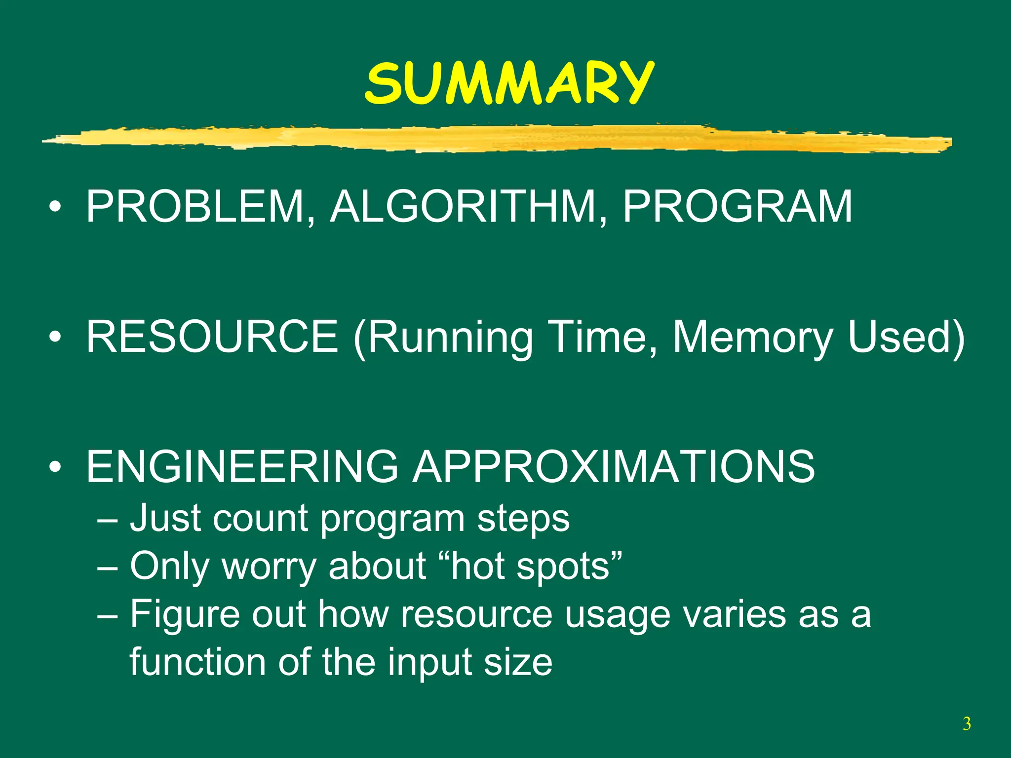
• PROBLEM, ALGORITHM,PROGRAM
• RESOURCE (Running Time, Memory Used)
• ENGINEERING APPROXIMATIONS
– Just count program steps
– Only worry about “hot spots”
– Figure out how resource usage varies as a
function of the input size
4.
4
MATHEMATICAL FRAMEWORK
• Establisha relative order among the growth
rate of functions.
• Use functions to model the “approximate”
and “asymptotic” (running time) behaviour of
algorithms.
5.
5
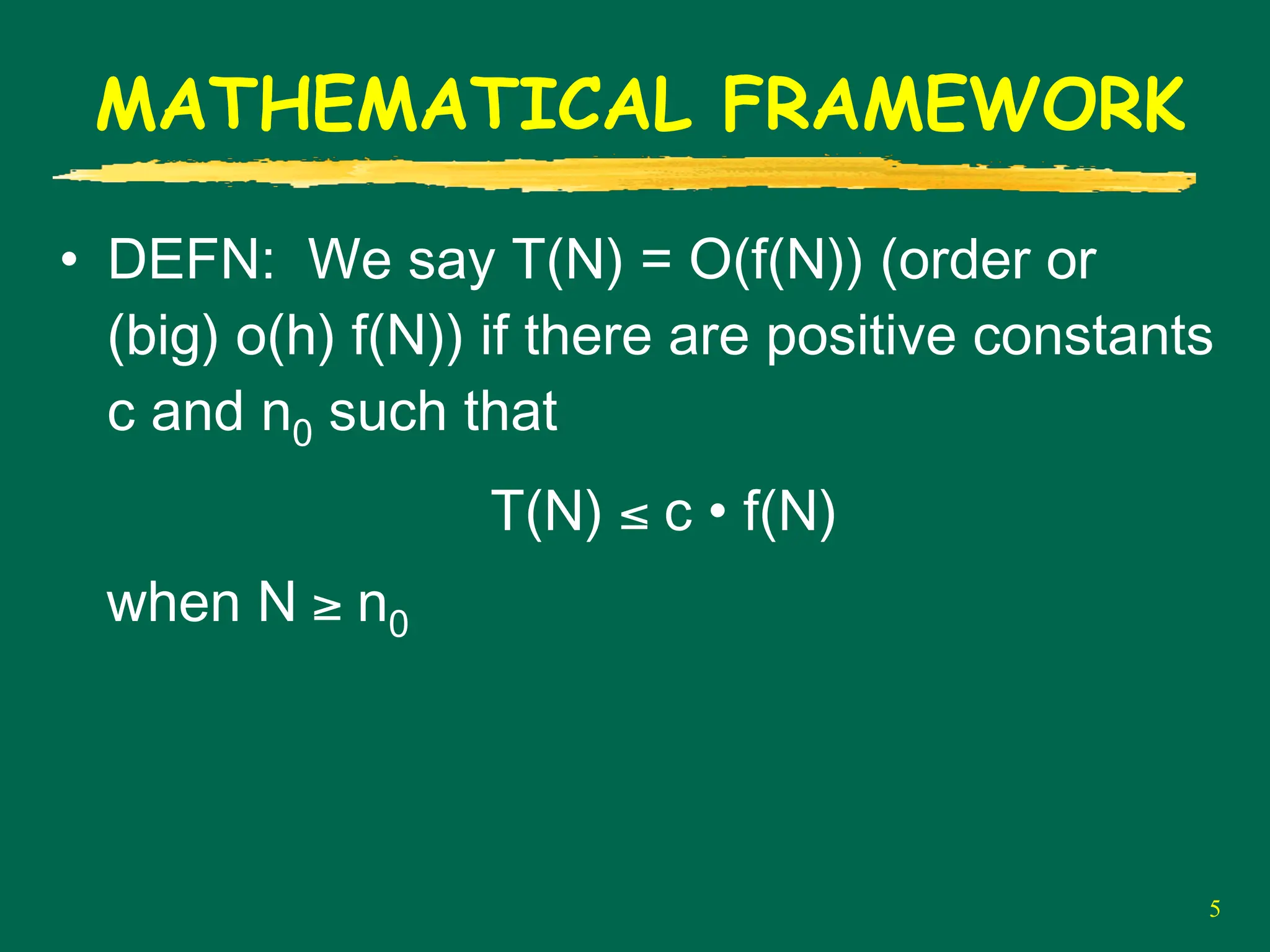
MATHEMATICAL FRAMEWORK
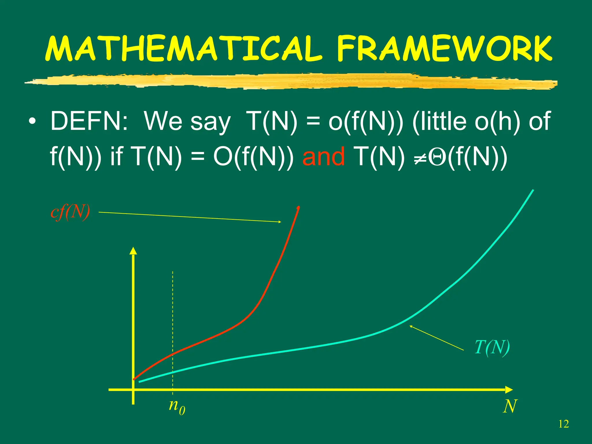
• DEFN:We say T(N) = O(f(N)) (order or
(big) o(h) f(N)) if there are positive constants
c and n0 such that
T(N) ≤ c • f(N)
when N ≥ n0
6.
6
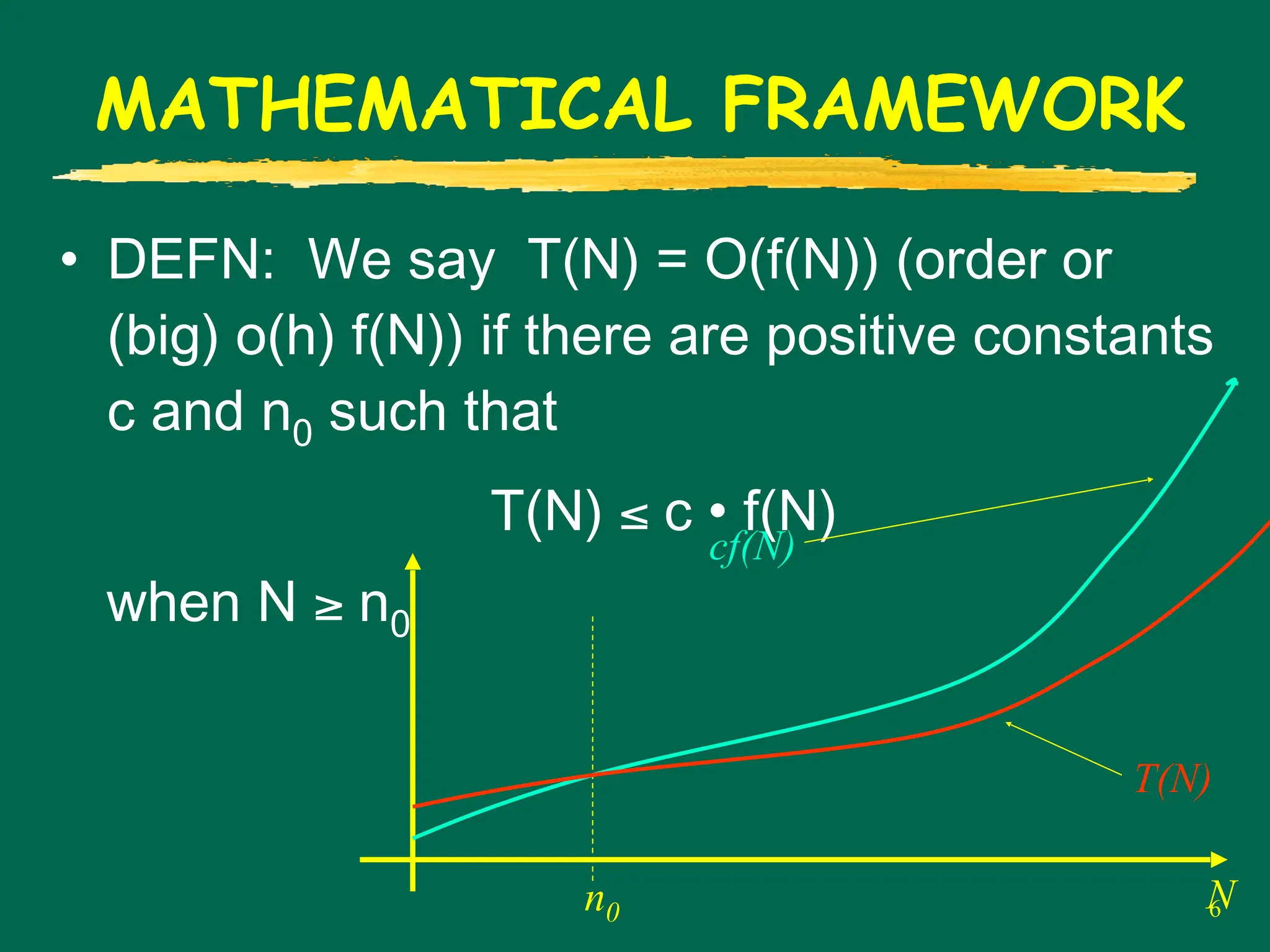
MATHEMATICAL FRAMEWORK
• DEFN:We say T(N) = O(f(N)) (order or
(big) o(h) f(N)) if there are positive constants
c and n0 such that
T(N) ≤ c • f(N)
when N ≥ n0
n0 N
cf(N)
T(N)
7.
7
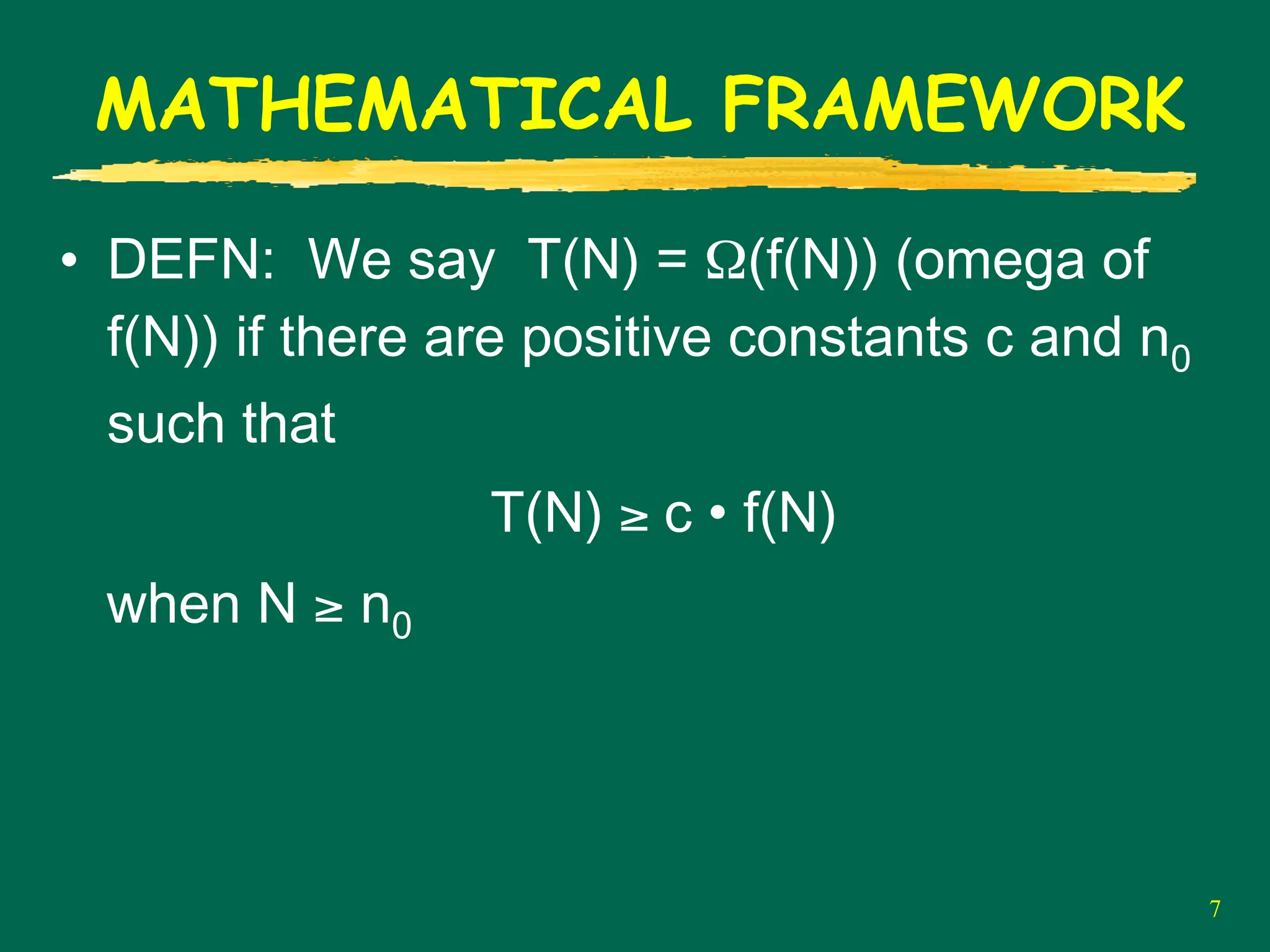
MATHEMATICAL FRAMEWORK
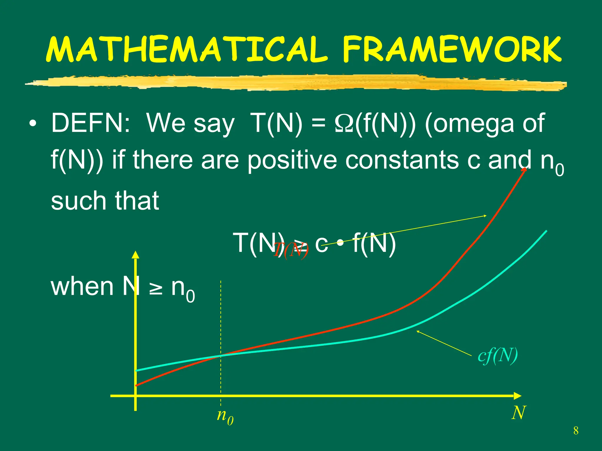
• DEFN:We say T(N) = Ω(f(N)) (omega of
f(N)) if there are positive constants c and n0
such that
T(N) ≥ c • f(N)
when N ≥ n0
8.
8
MATHEMATICAL FRAMEWORK
• DEFN:We say T(N) = Ω(f(N)) (omega of
f(N)) if there are positive constants c and n0
such that
T(N) ≥ c • f(N)
when N ≥ n0
n0 N
cf(N)
T(N)
13
EXAMPLES
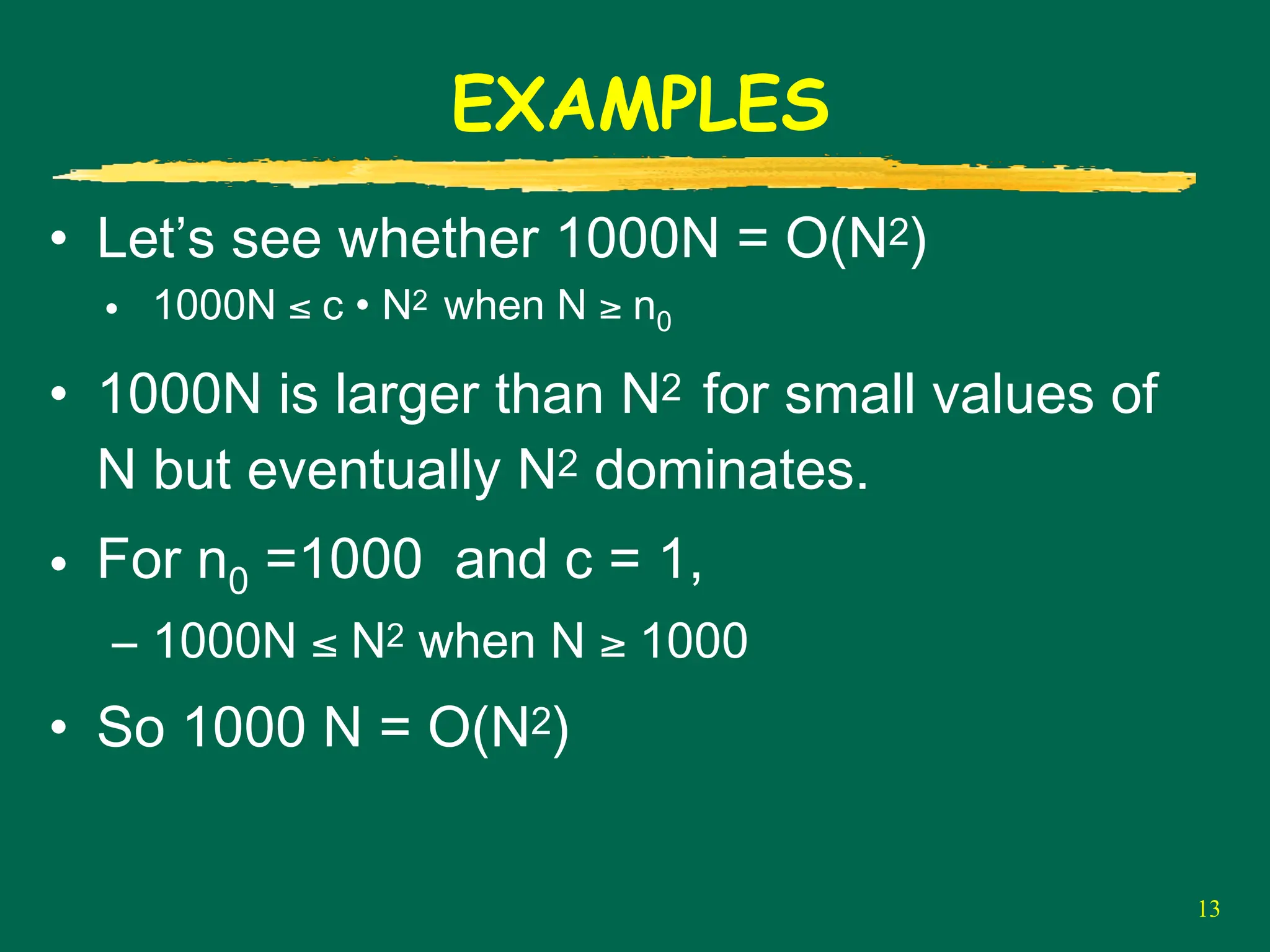
• Let’s seewhether 1000N = O(N2)
• 1000N ≤ c • N2 when N ≥ n0
• 1000N is larger than N2 for small values of
N but eventually N2 dominates.
• For n0 =1000 and c = 1,
– 1000N ≤ N2 when N ≥ 1000
• So 1000 N = O(N2)
14.
14
EXAMPLES
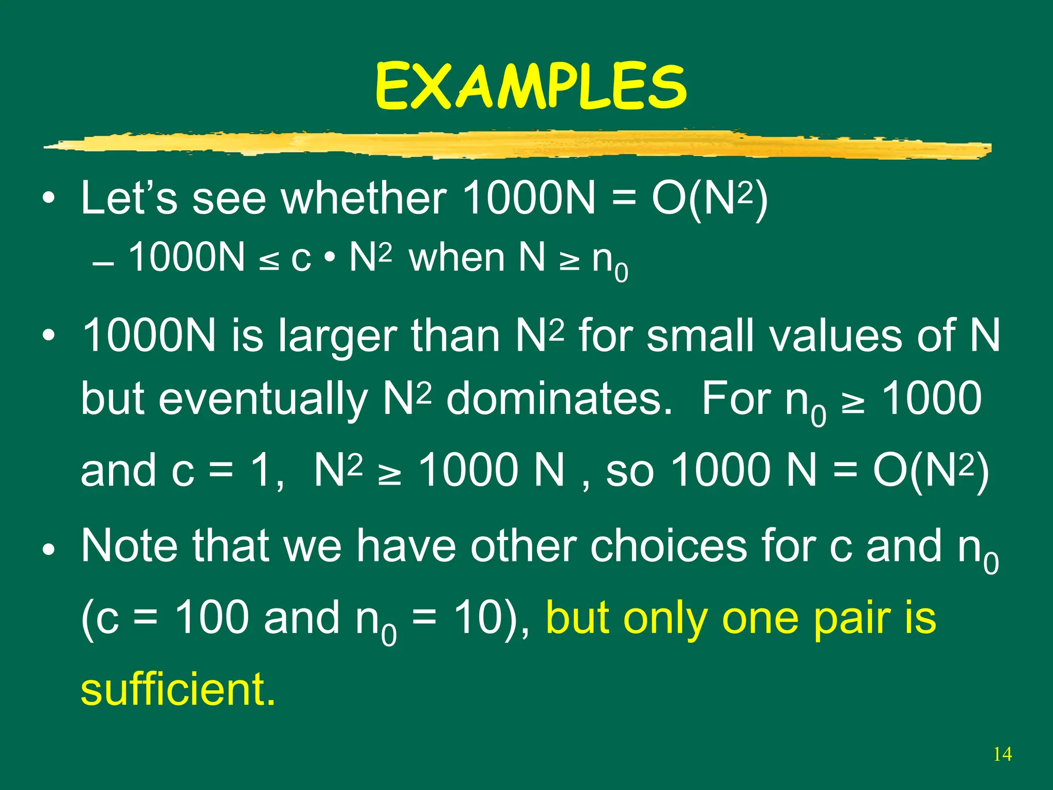
• Let’s seewhether 1000N = O(N2)
– 1000N ≤ c • N2 when N ≥ n0
• 1000N is larger than N2 for small values of N
but eventually N2 dominates. For n0 ≥ 1000
and c = 1, N2 ≥ 1000 N , so 1000 N = O(N2)
• Note that we have other choices for c and n0
(c = 100 and n0 = 10), but only one pair is
sufficient.
15.
15
EXAMPLES
• 1000N =O(N2)
• 1000N is larger than N2 for small values of N but
eventually N2 dominates. For n0 ≥ 1000 and c =
1, N2 ≥ 1000 N , so 1000 N = O(N2)
• Note that we have other choices for c and n0 (c
= 100 and n0 = 10), but only one pair is sufficient.
• Basically what we are saying is that 1000N grows
slower than N2.
16.
16
EXAMPLES
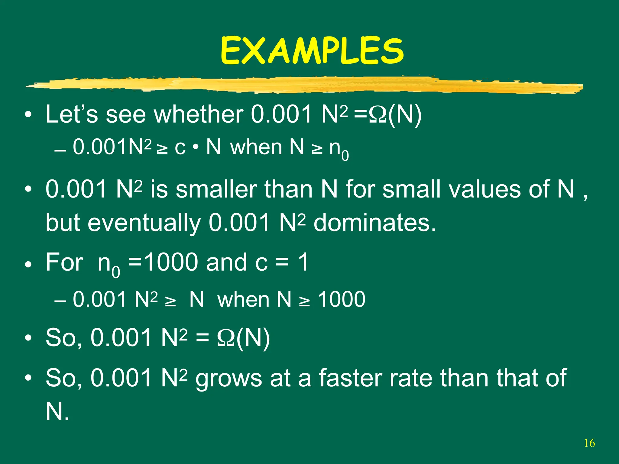
• Let’s seewhether 0.001 N2 =Ω(N)
– 0.001N2 ≥ c • N when N ≥ n0
• 0.001 N2 is smaller than N for small values of N ,
but eventually 0.001 N2 dominates.
• For n0 =1000 and c = 1
– 0.001 N2 ≥ N when N ≥ 1000
• So, 0.001 N2 = Ω(N)
• So, 0.001 N2 grows at a faster rate than that of
N.
19
EXAMPLES
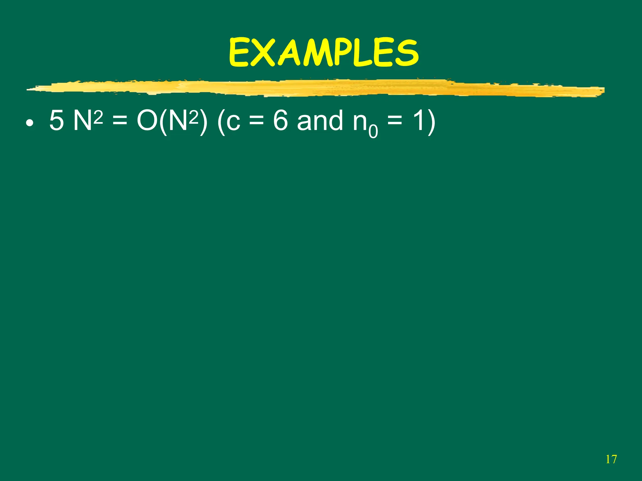
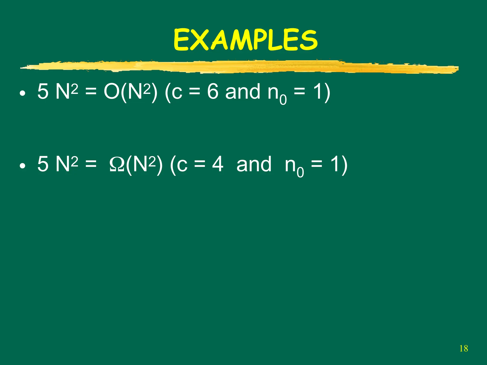
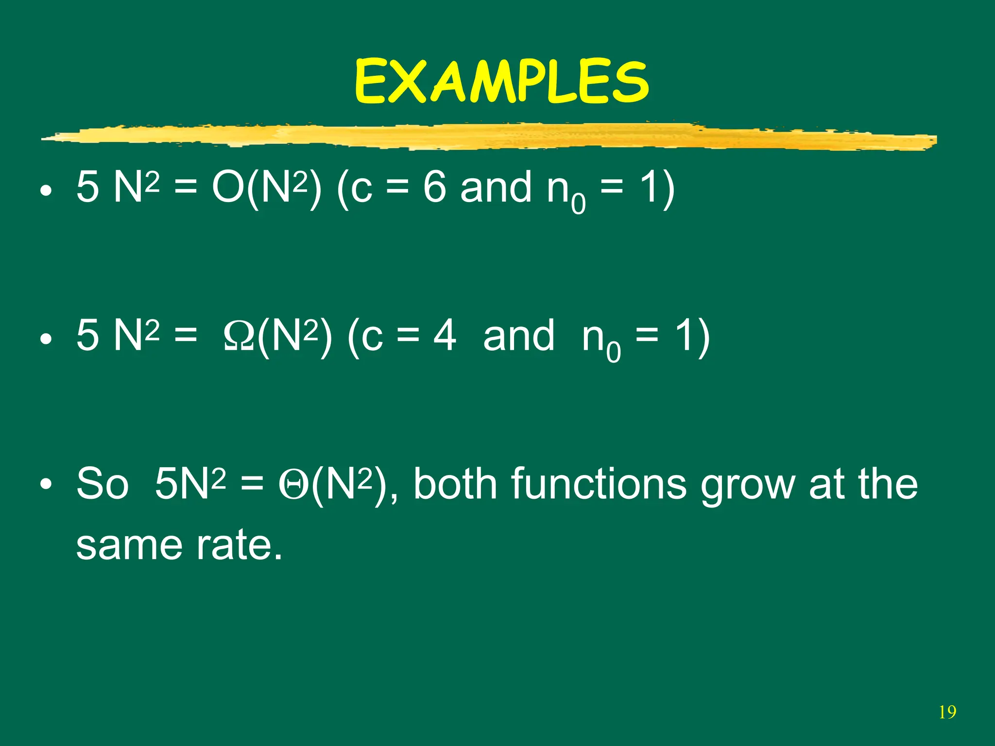
• 5 N2= O(N2) (c = 6 and n0 = 1)
• 5 N2 = Ω(N2) (c = 4 and n0 = 1)
• So 5N2 = Θ(N2), both functions grow at the
same rate.
20.
20
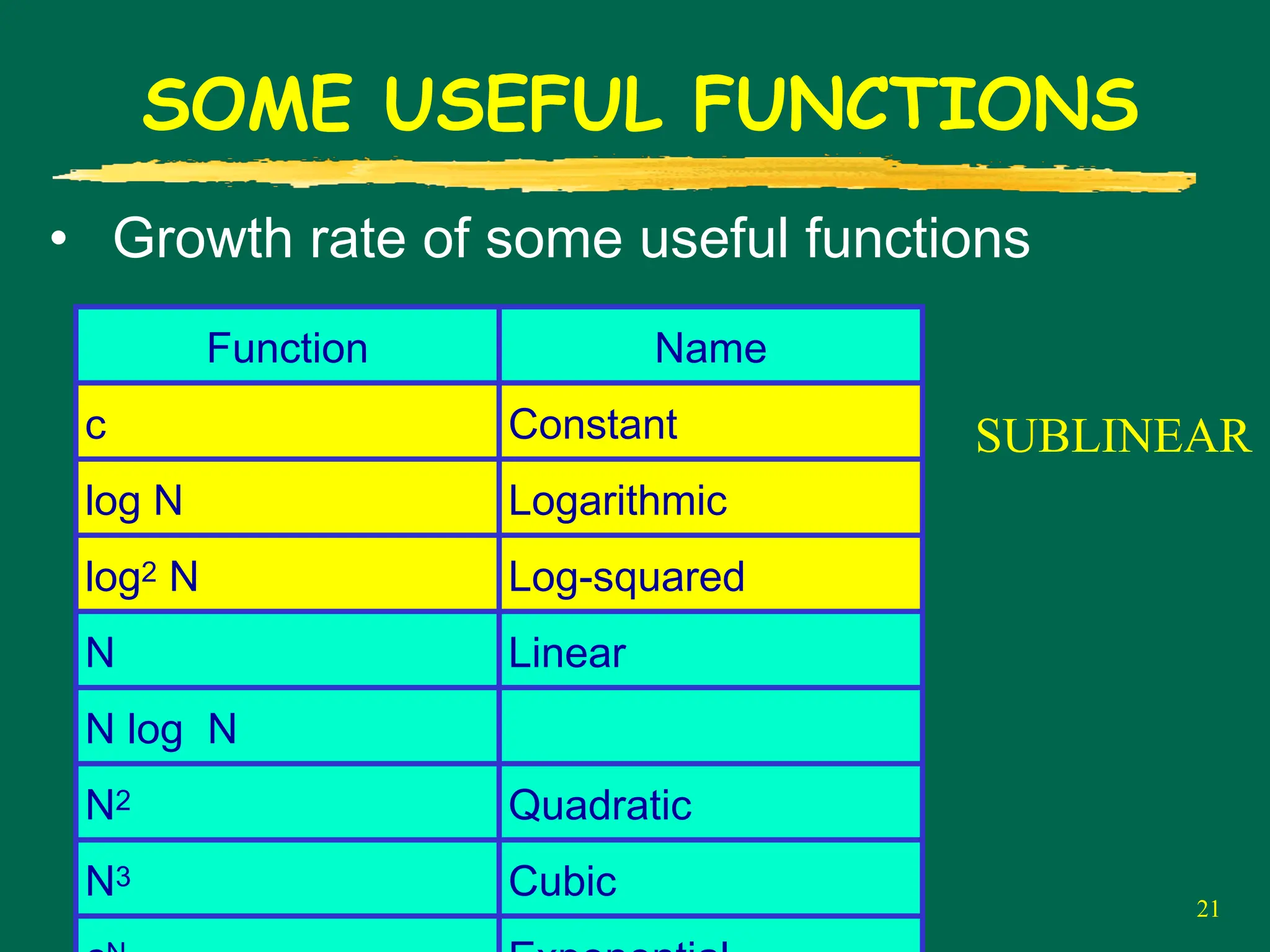
SOME USEFUL FUNCTIONS
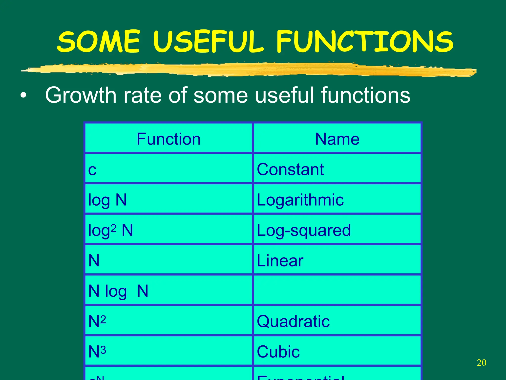
•Growth rate of some useful functions
Function Name
c Constant
log N Logarithmic
log2 N Log-squared
N Linear
N log N
N2 Quadratic
N3 Cubic
21.
21
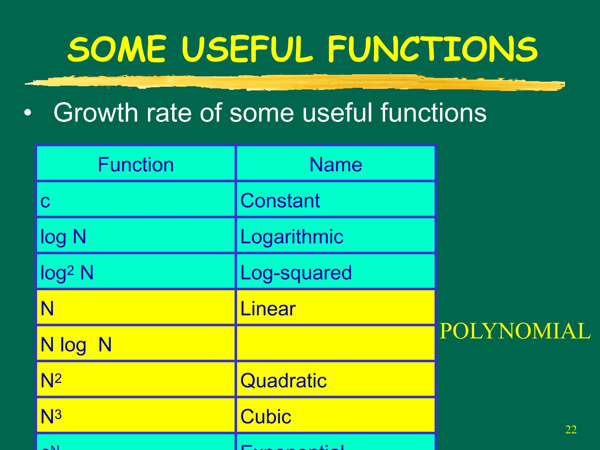
SOME USEFUL FUNCTIONS
•Growth rate of some useful functions
Function Name
c Constant
log N Logarithmic
log2 N Log-squared
N Linear
N log N
N2 Quadratic
N3 Cubic
SUBLINEAR
22.
22
SOME USEFUL FUNCTIONS
•Growth rate of some useful functions
Function Name
c Constant
log N Logarithmic
log2 N Log-squared
N Linear
N log N
N2 Quadratic
N3 Cubic
POLYNOMIAL
24
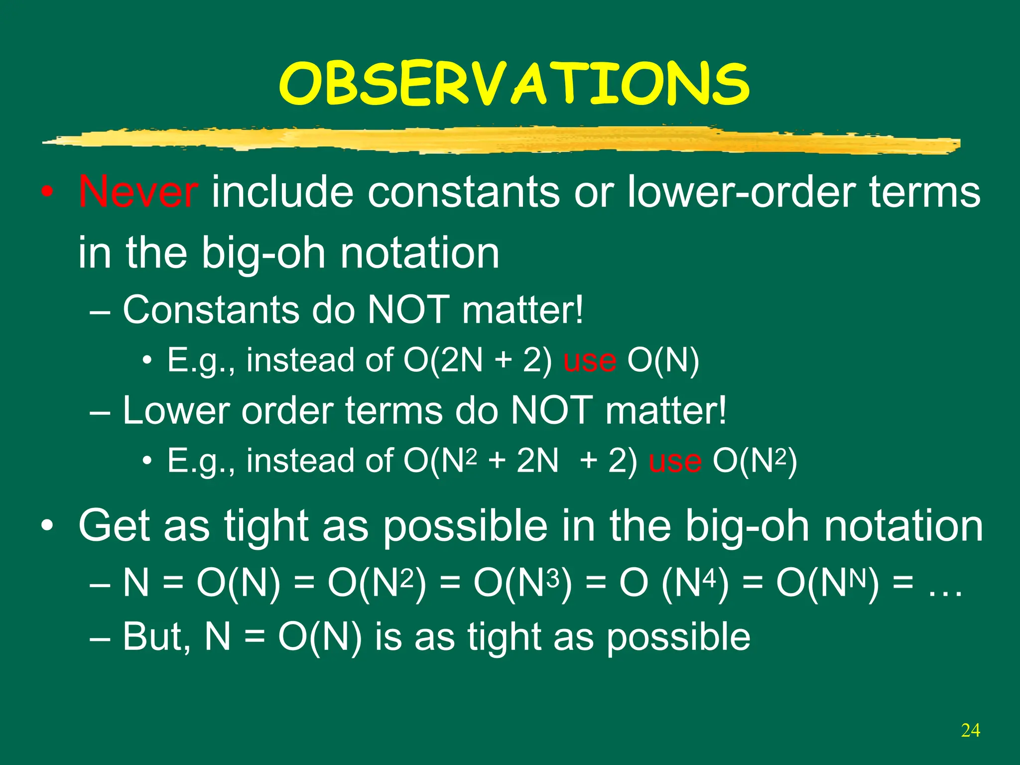
OBSERVATIONS
• Never includeconstants or lower-order terms
in the big-oh notation
– Constants do NOT matter!
• E.g., instead of O(2N + 2) use O(N)
– Lower order terms do NOT matter!
• E.g., instead of O(N2 + 2N + 2) use O(N2)
• Get as tight as possible in the big-oh notation
– N = O(N) = O(N2) = O(N3) = O (N4) = O(NN) = …
– But, N = O(N) is as tight as possible
25.
25
RULES
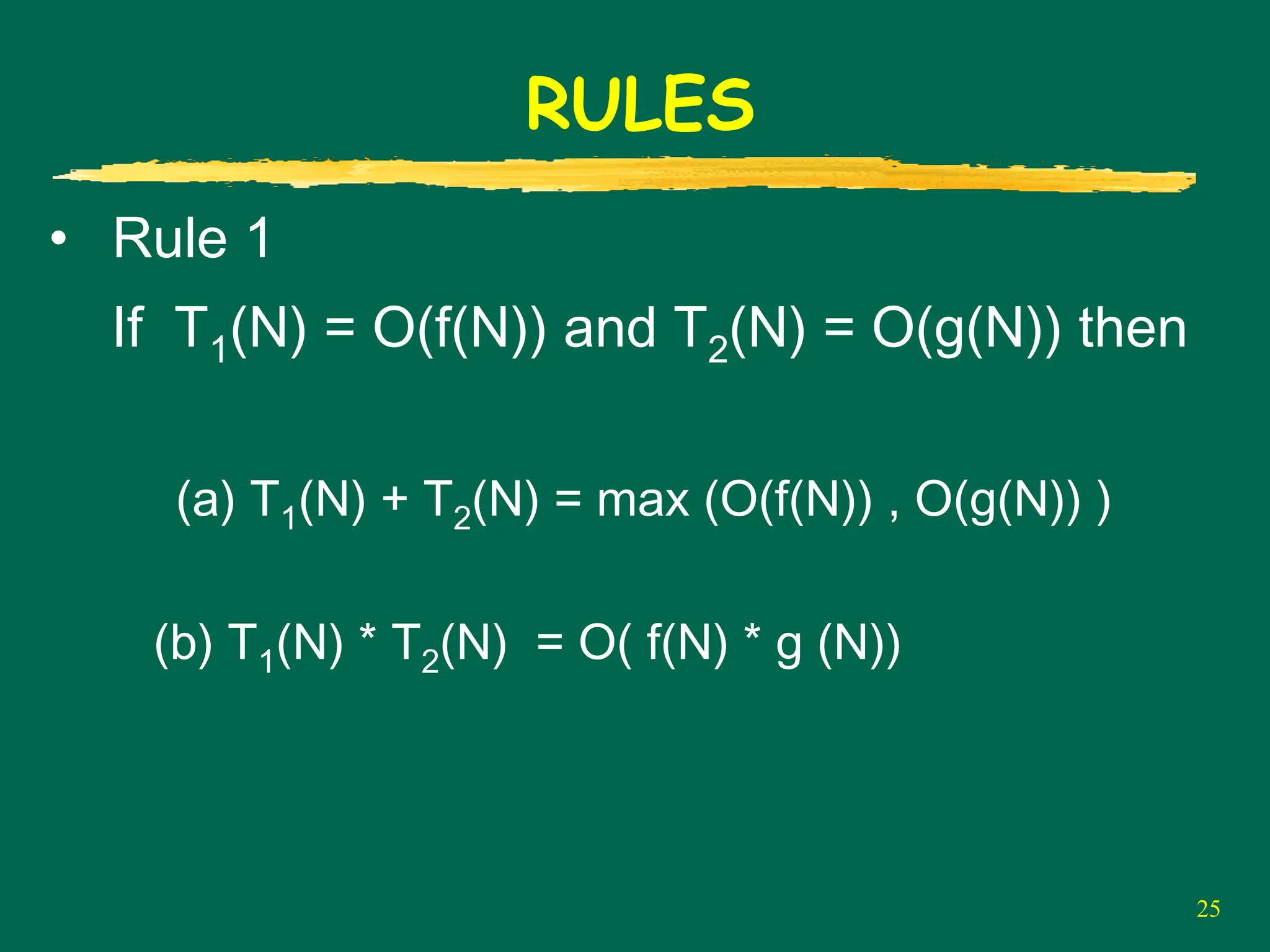
• Rule 1
IfT1(N) = O(f(N)) and T2(N) = O(g(N)) then
(a) T1(N) + T2(N) = max (O(f(N)) , O(g(N)) )
(b) T1(N) * T2(N) = O( f(N) * g (N))
28
ANALYZING COMPLEXITY
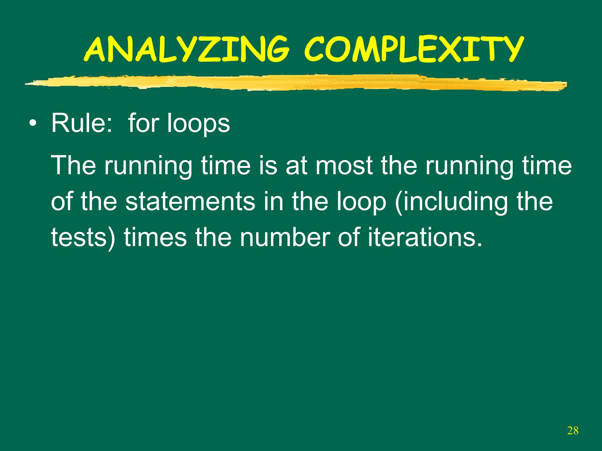
• Rule:for loops
The running time is at most the running time
of the statements in the loop (including the
tests) times the number of iterations.
29.
29
ANALYZING COMPLEXITY
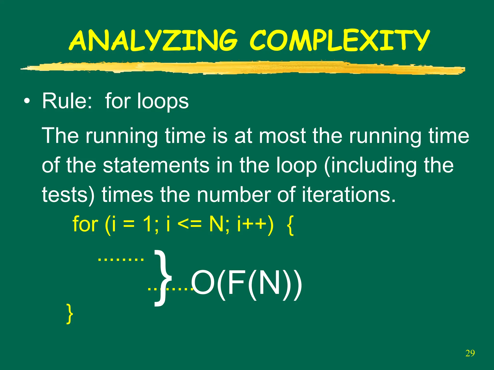
• Rule:for loops
The running time is at most the running time
of the statements in the loop (including the
tests) times the number of iterations.
for (i = 1; i <= N; i++) {
........
........
}
} O(F(N))
30.
30
ANALYZING COMPLEXITY
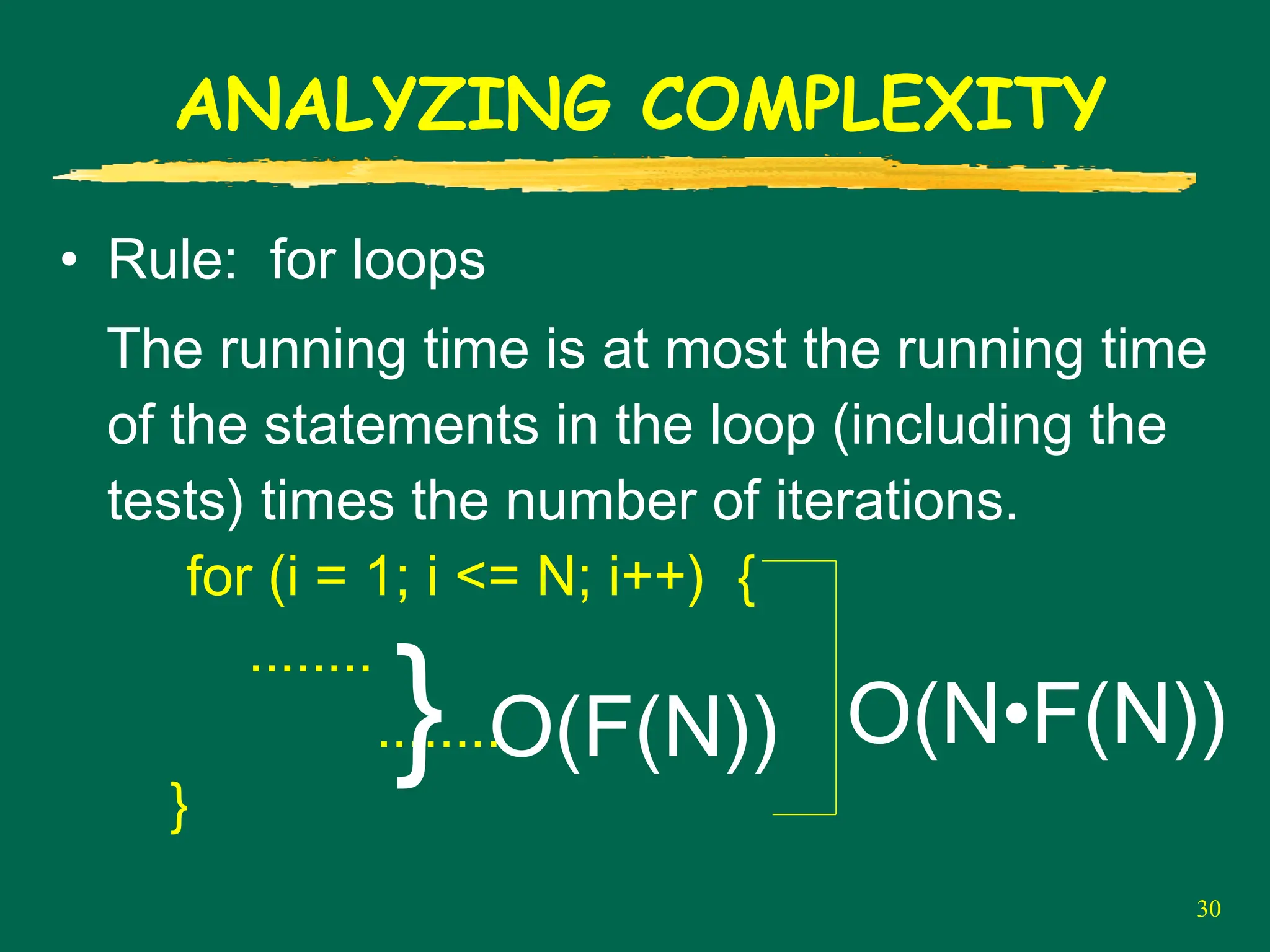
• Rule:for loops
The running time is at most the running time
of the statements in the loop (including the
tests) times the number of iterations.
for (i = 1; i <= N; i++) {
........
........
}
} O(F(N)) O(N•F(N))
31.
31
ANALYZING COMPLEXITY
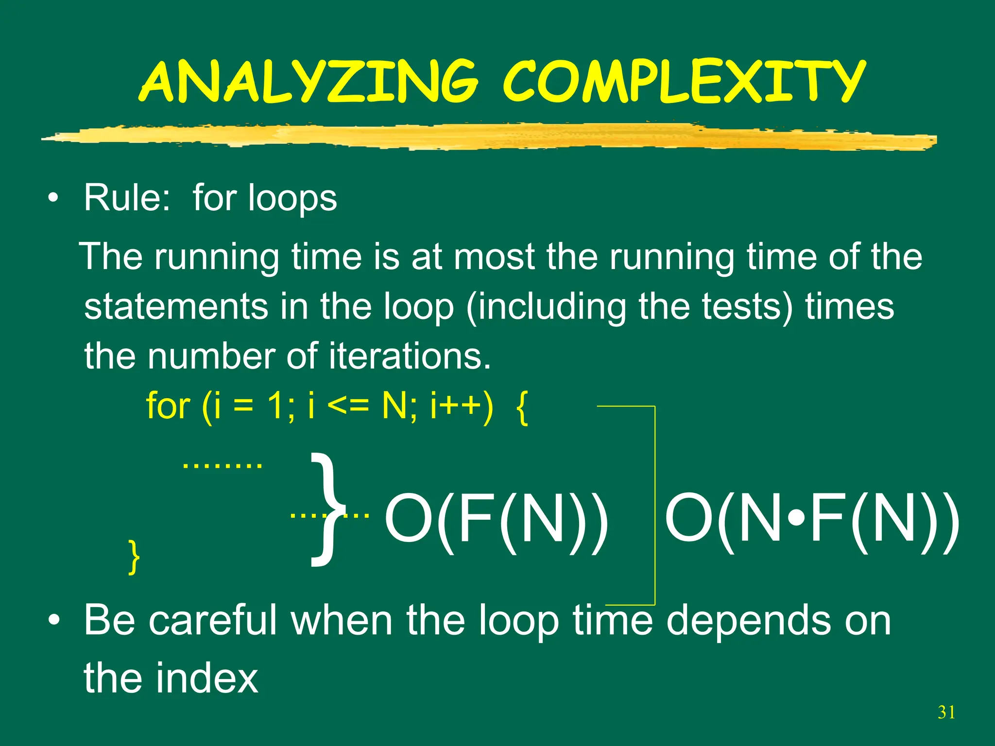
• Rule:for loops
The running time is at most the running time of the
statements in the loop (including the tests) times
the number of iterations.
for (i = 1; i <= N; i++) {
........
........
}
• Be careful when the loop time depends on
the index
} O(F(N)) O(N•F(N))
32.
32
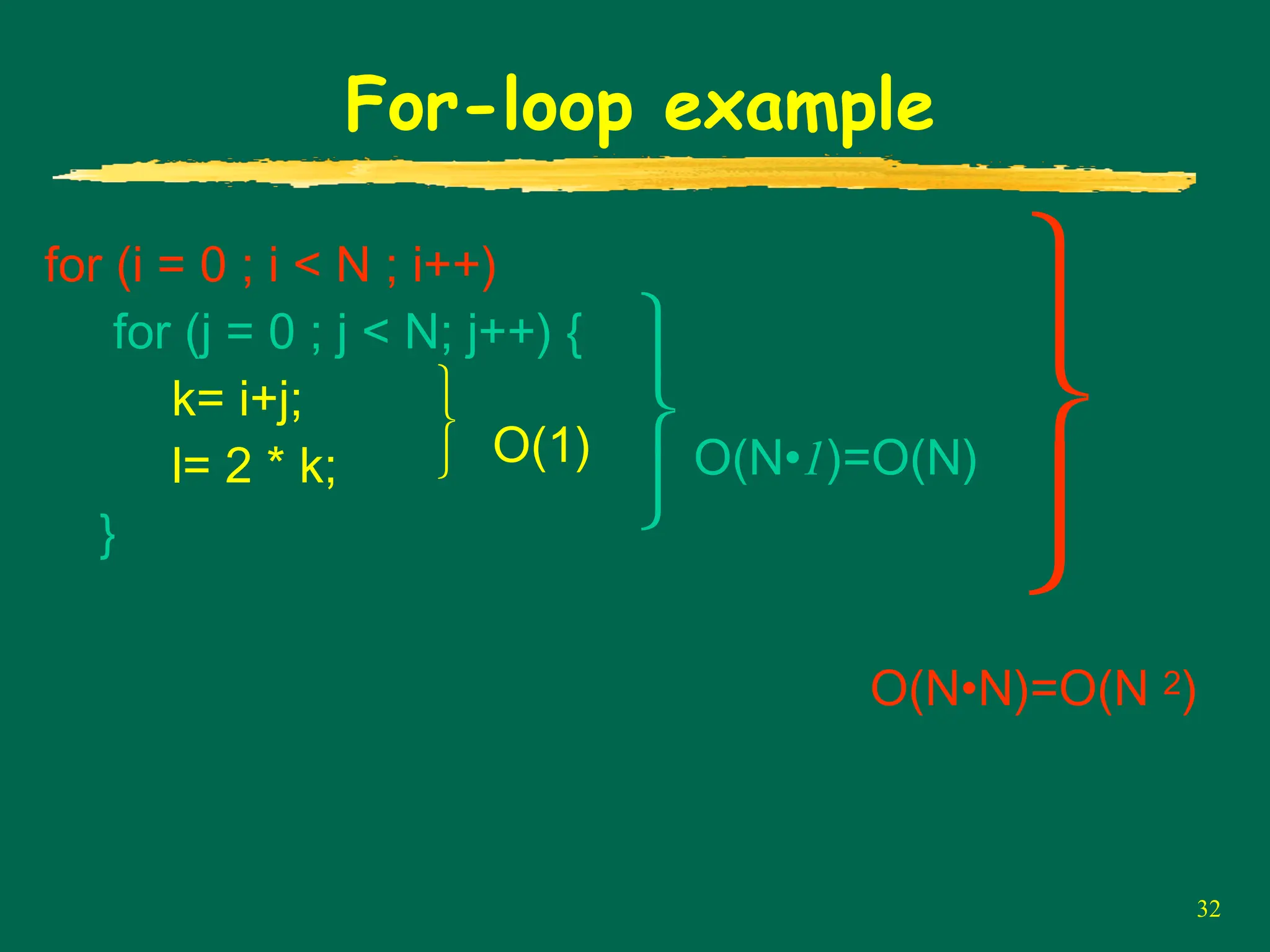
For-loop example
for (i= 0 ; i < N ; i++)
for (j = 0 ; j < N; j++) {
k= i+j;
l= 2 * k;
}
O(1)
⎫
⎬
⎭ O(N•1)=O(N)
⎫
⎬
⎭
O(N•N)=O(N 2)
⎫
⎬
⎭
33.
33
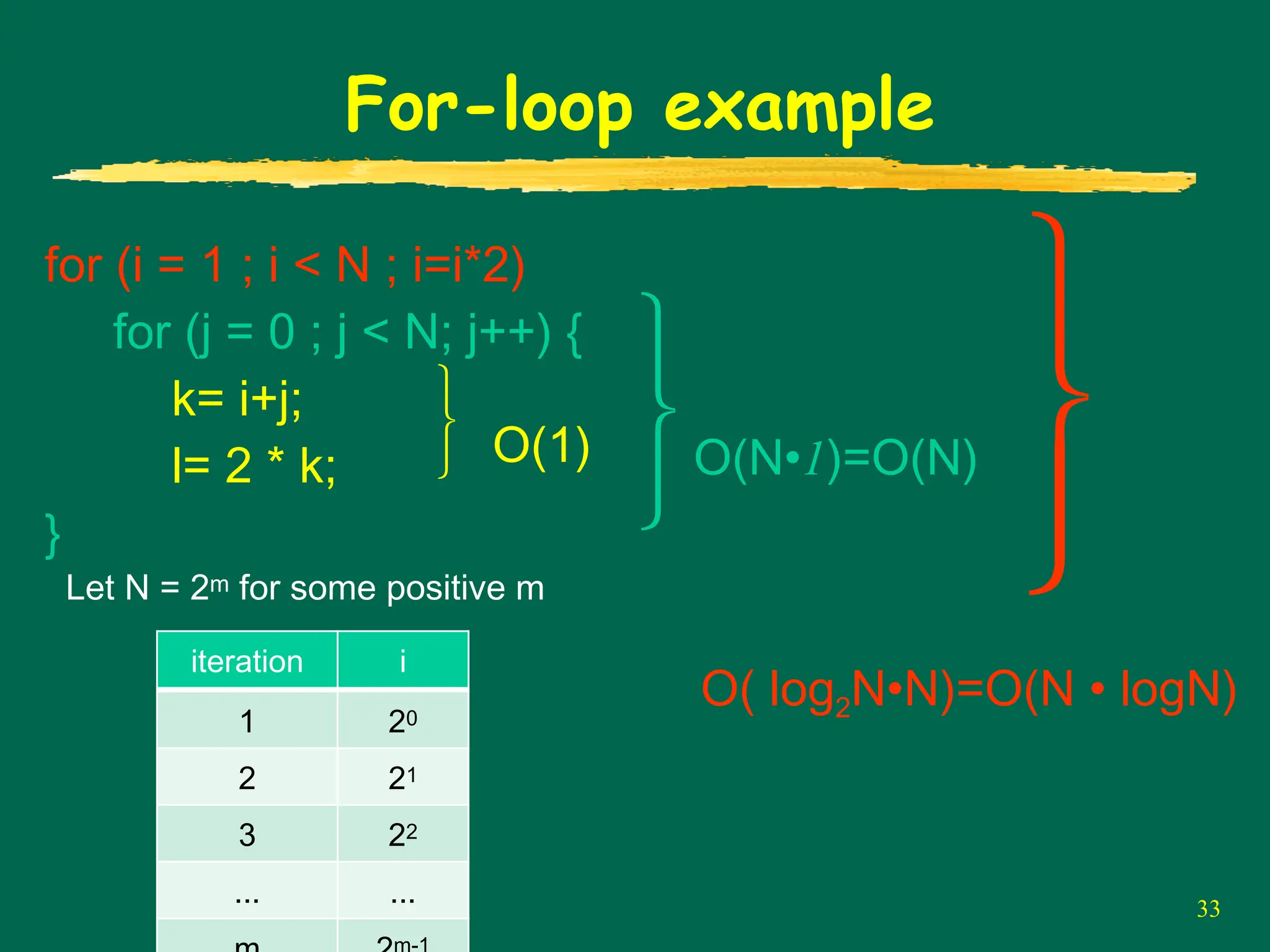
For-loop example
for (i= 1 ; i < N ; i=i*2)
for (j = 0 ; j < N; j++) {
k= i+j;
l= 2 * k;
}
O(1)
⎫
⎬
⎭ O(N•1)=O(N)
⎫
⎬
⎭
O( log2N•N)=O(N • logN)
⎫
⎬
⎭
Let N = 2m for some positive m
iteration i
1 20
2 21
3 22
... ...
34.
34
ANALYZING COMPLEXITY
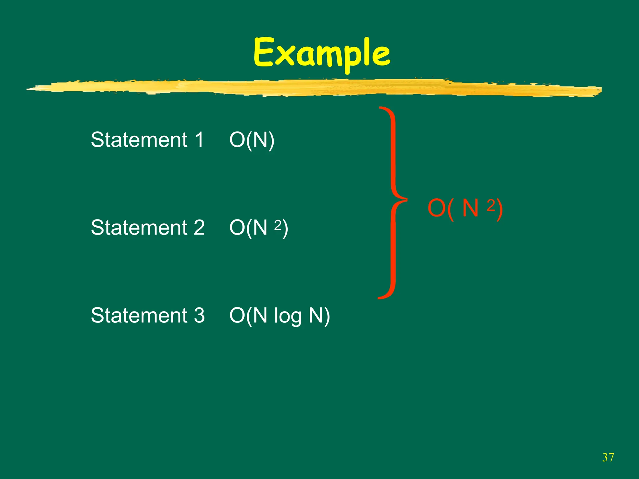
• Rule:Consecutive Statements
– The running time is the sum of the running times
of individual statements
35.
35
ANALYZING COMPLEXITY
• Rule:Consecutive Statements
– The running time is the sum of the running times
of individual statements
• Remember that
If T1(N) = O(f(N)) and T2(N) = O(g(N)) then
T1(N) + T2(N) = max (O(f(N)) , O(g(N)) )
36.
36
ANALYZING COMPLEXITY
• Rule:Consecutive Statements
– The running time is the sum of the running times of
individual statements,
• Remember that
If T1(N) = O(f(N)) and T2(N) = O(g(N)) then
T1(N) + T2(N) = max (O(f(N)) , O(g(N)) )
• Which means that you have to take the
maximum of the running times of the
statements.
38
ANALYZING COMPLEXITY
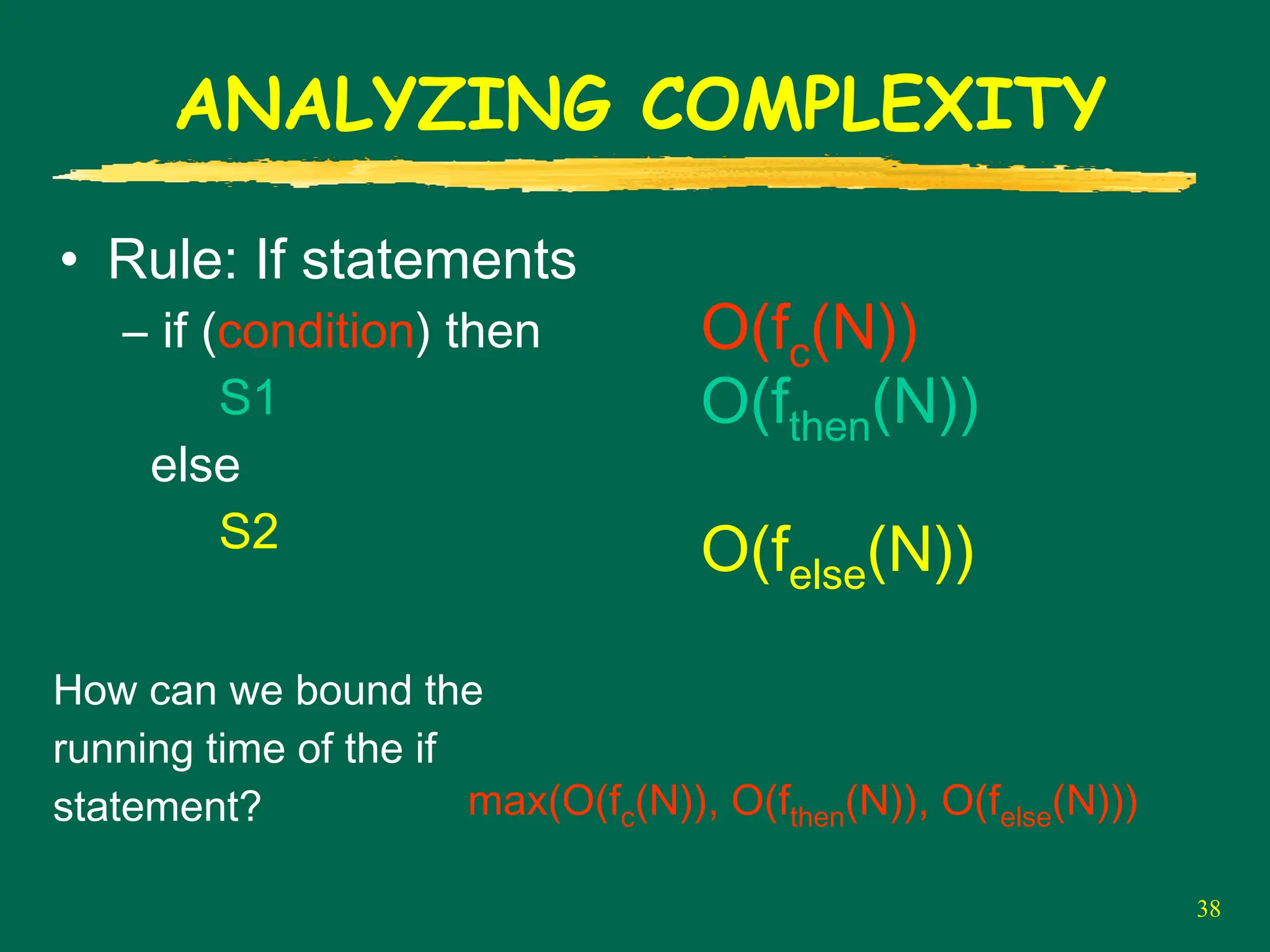
• Rule:If statements
– if (condition) then
S1
else
S2
O(fc(N))
O(fthen(N))
O(felse(N))
How can we bound the
running time of the if
statement? max(O(fc(N)), O(fthen(N)), O(felse(N)))
39.
39
AN EXAMPLE
{
1 inti,j;
2 for(i=1; i <= n ; i=i*2) {
3 for(j = 0; j < i; j++) {
4 foo[i][j] = 0;
5 for (k = 0; k < n; k++) {
6 foo[i][j] = bar[k][i+j] + foo[i][j];
7 }
8 }
9 }
}
O(1) O(n)
O(1)
O(n)
40.
40
AN EXAMPLE
{
1 inti,j;
2 for(i=1; i <= n ; i=i*2) {
3 for(j = 0; j < i; j++) {
4 foo[i][j] = 0;
5 for (k = 0; k < n; k++) {
6 foo[i][j] = bar[k][i+j] + foo[i][j];
7 }
8 }
9 }
}
O(n)
O(i•n)
41.
41
AN EXAMPLE
{
1 inti,j;
2 for(i=1; i <= n ; i=i*2) {
3 for(j = 0; j < i; j++) {
4 foo[i][j] = 0;
5 for (k = 0; k < n; k++) {
6 foo[i][j] = bar[k][i+j] + foo[i][j];
7 }
8 }
9 }
}
O(n)
O(i•n)
Although this loop is executed about log n times,
at each iteration the time of the inner loop
changes!
42.
42
AN EXAMPLE
{
1 inti,j;
2 for(i=1; i <= n ; i=i*2) {
3 for(j = 0; j < i; j++) {
4 foo[i][j] = 0;
5 for (k = 0; k < n; k++) {
6 foo[i][j] = bar[k][i+j] + foo[i][j];
7 }
8 }
9 }
}
O(n)
O(i•n)
Although this loop is executed about log n times,
at each iteration the time of the inner loop
changes!
43.
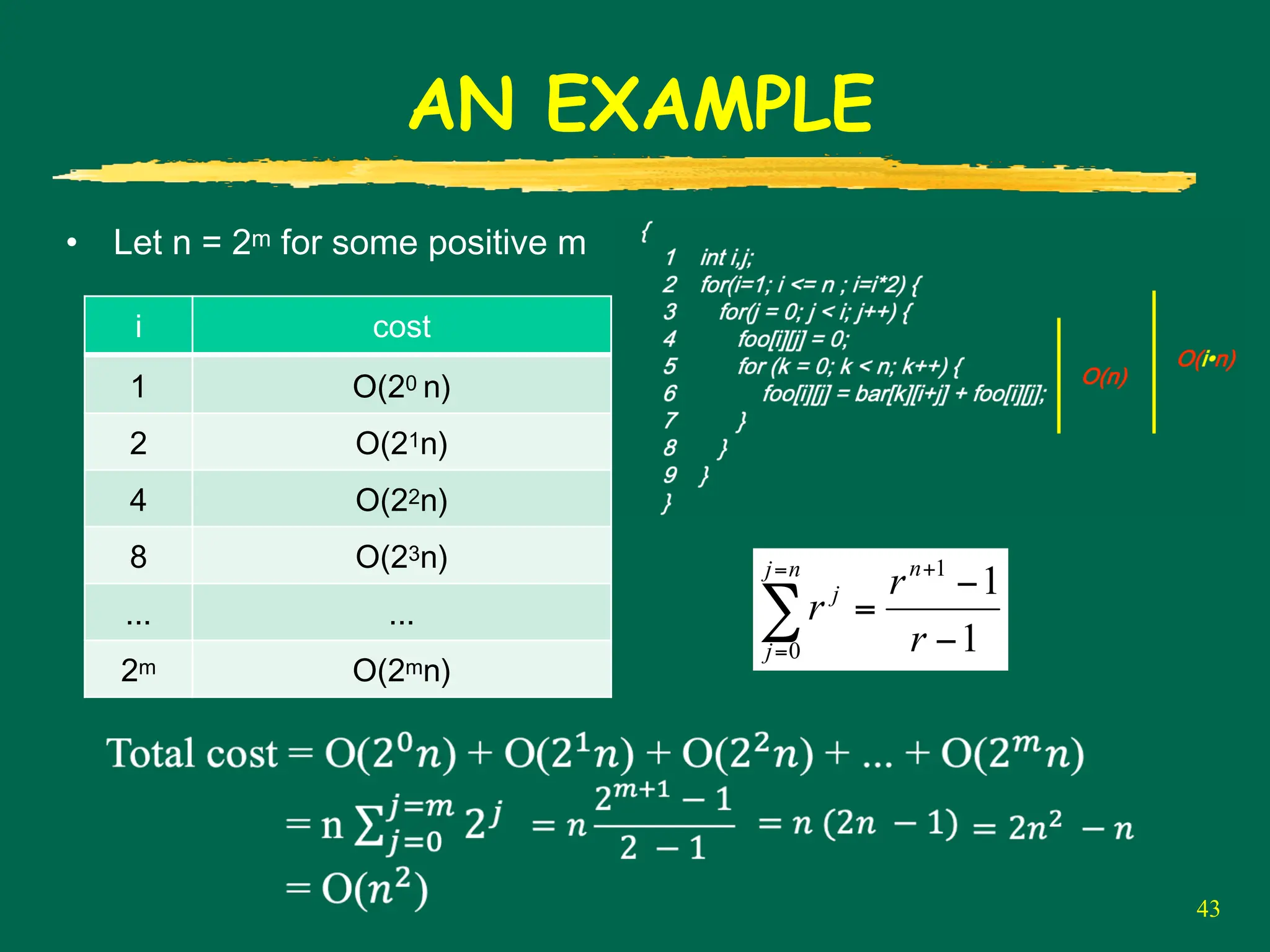
AN EXAMPLE
43
i cost
1O(20 n)
2 O(21n)
4 O(22n)
8 O(23n)
... ...
2m O(2mn)
• Let n = 2m for some positive m
1
1
1
0 −
−
=
+
=
=
∑ r
r
r
n
n
j
j
j
45
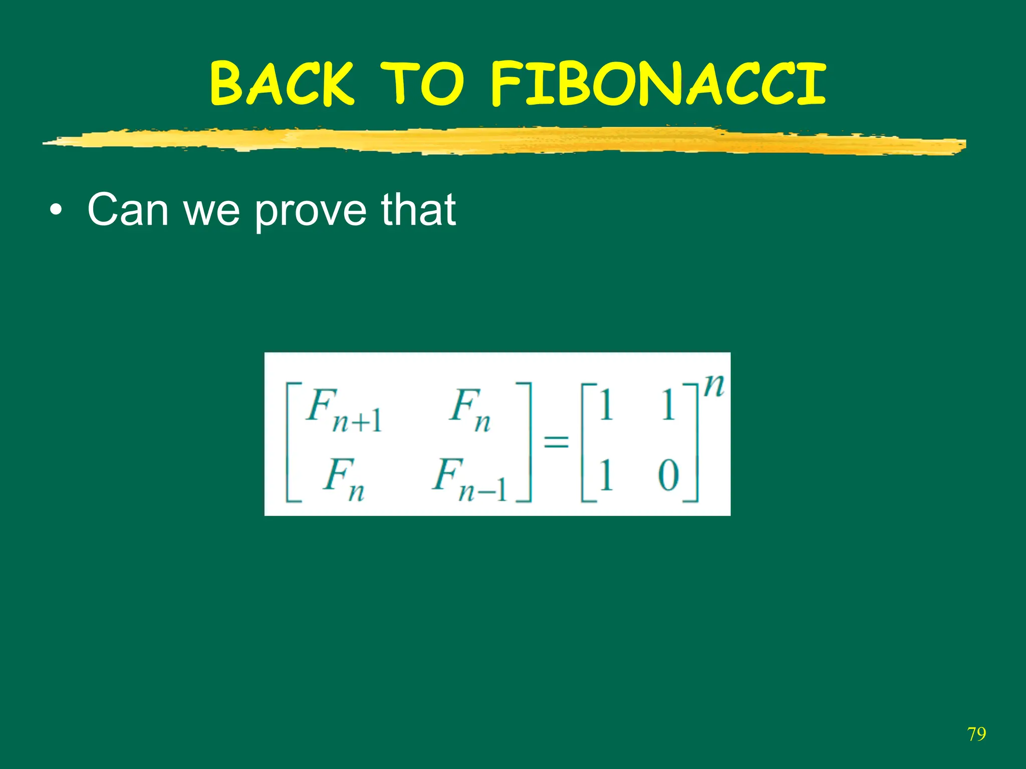
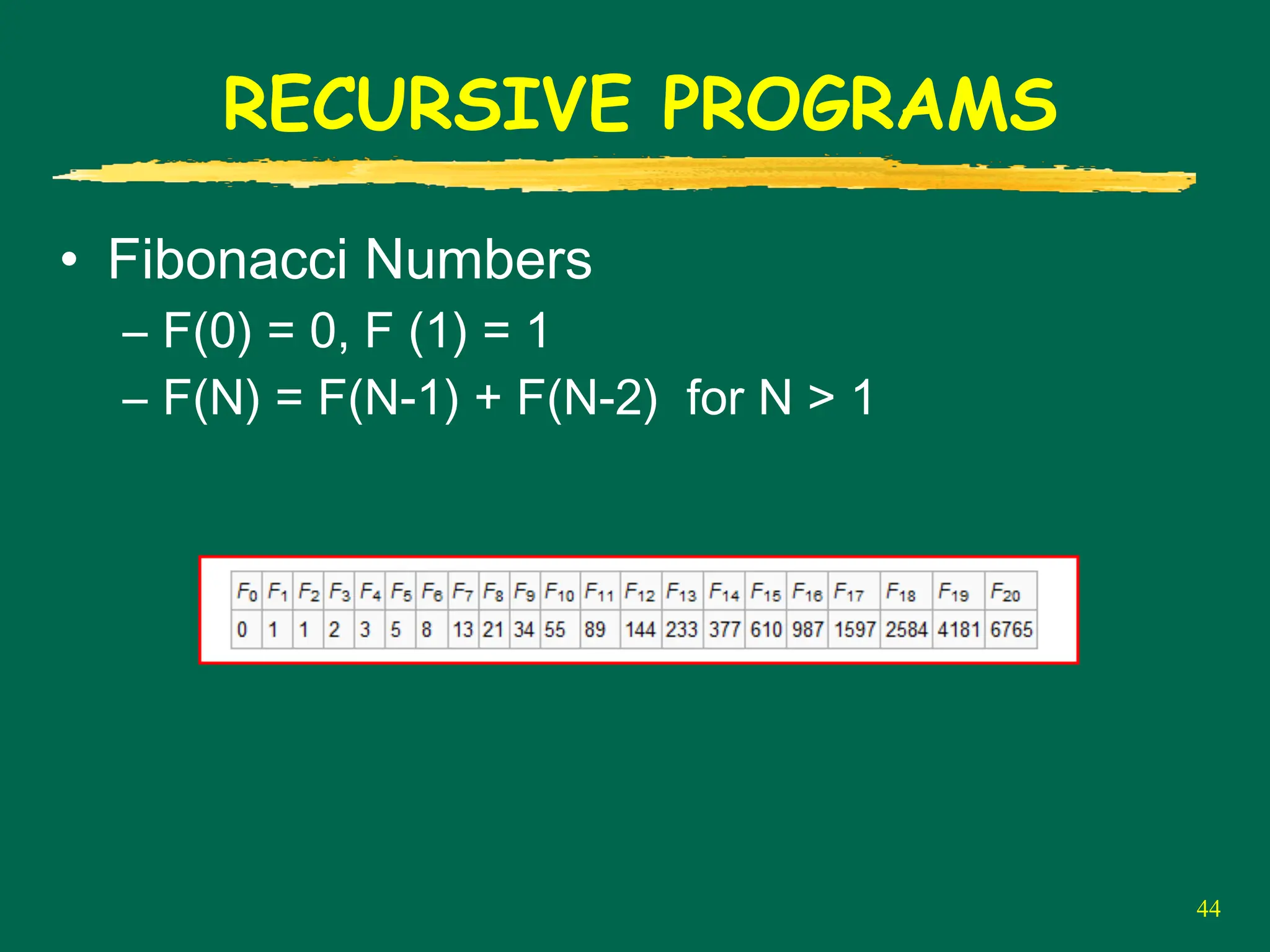
RECURSIVE PROGRAMS
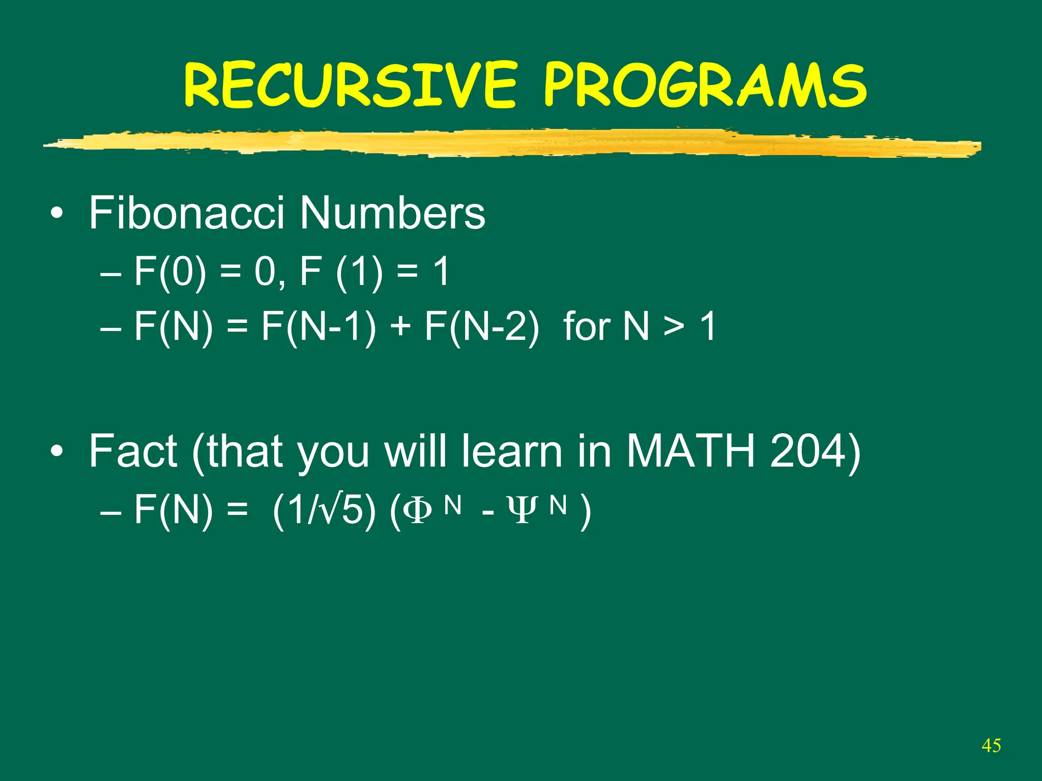
• FibonacciNumbers
– F(0) = 0, F (1) = 1
– F(N) = F(N-1) + F(N-2) for N > 1
• Fact (that you will learn in MATH 204)
– F(N) = (1/√5) (Φ N - Ψ N )
46.
46
RECURSIVE PROGRAMS
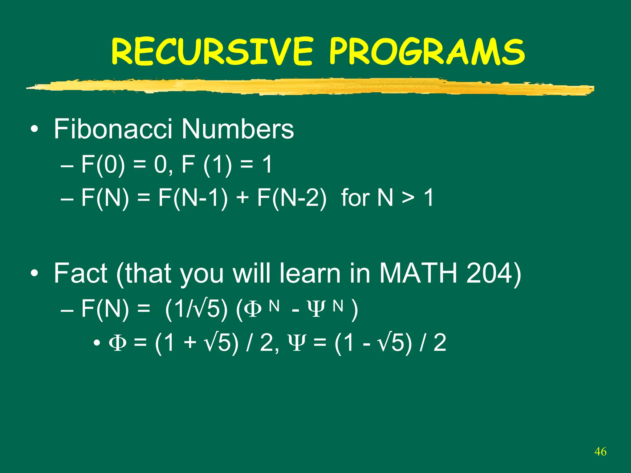
• FibonacciNumbers
– F(0) = 0, F (1) = 1
– F(N) = F(N-1) + F(N-2) for N > 1
• Fact (that you will learn in MATH 204)
– F(N) = (1/√5) (Φ N - Ψ N )
• Φ = (1 + √5) / 2, Ψ = (1 - √5) / 2
47.
47
RECURSIVE PROGRAMS
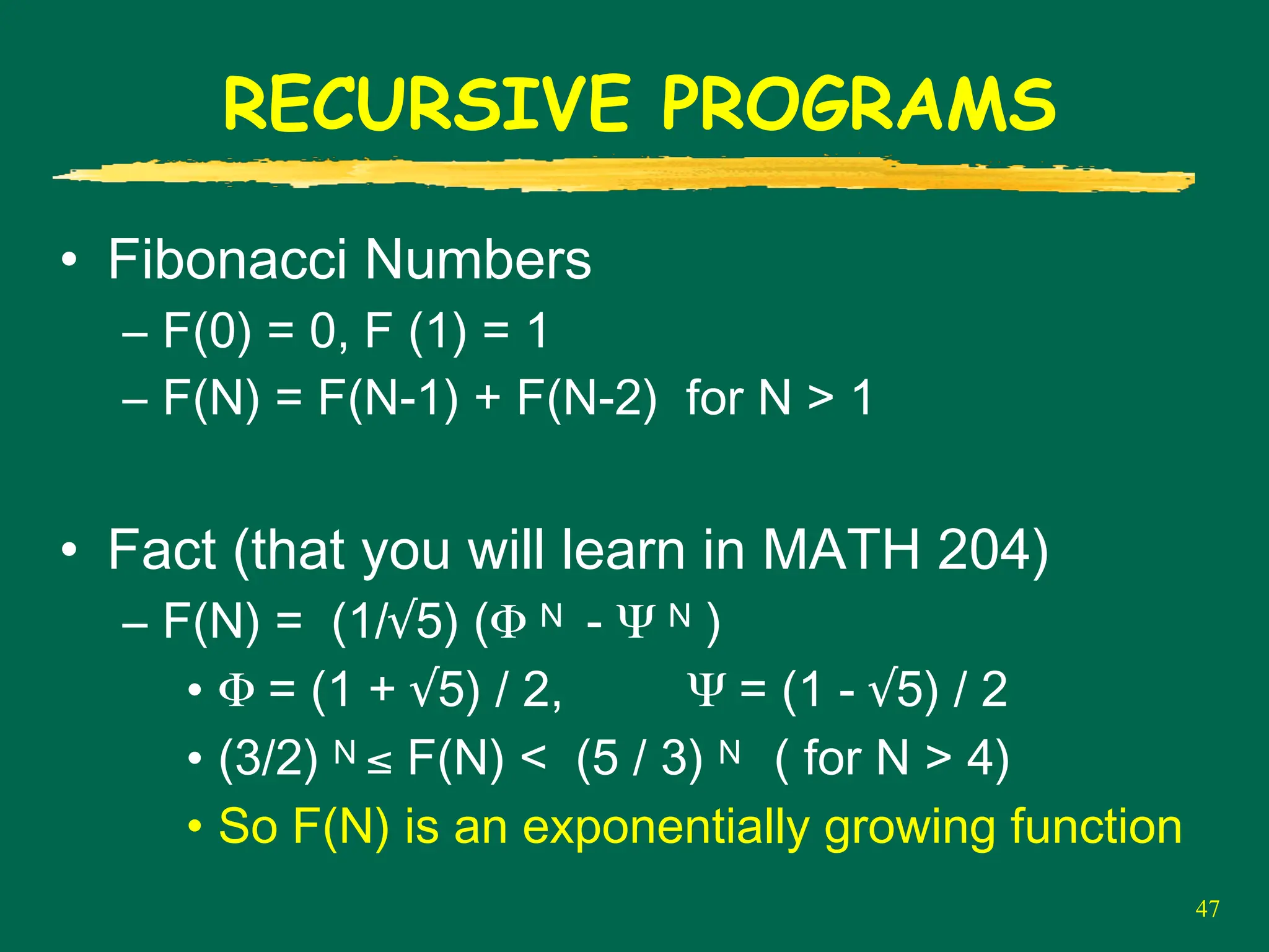
• FibonacciNumbers
– F(0) = 0, F (1) = 1
– F(N) = F(N-1) + F(N-2) for N > 1
• Fact (that you will learn in MATH 204)
– F(N) = (1/√5) (Φ N - Ψ N )
• Φ = (1 + √5) / 2, Ψ = (1 - √5) / 2
• (3/2) N ≤ F(N) < (5 / 3) N ( for N > 4)
• So F(N) is an exponentially growing function
48.
48
COMPUTING FIBONACCI NUMBERS
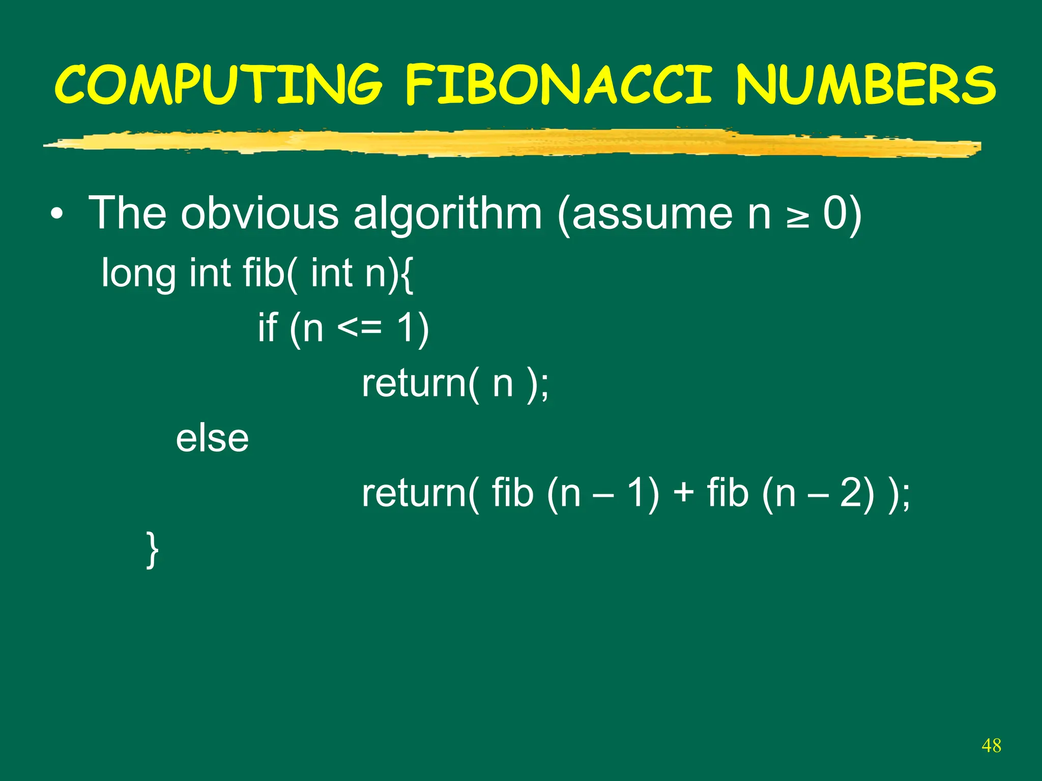
•The obvious algorithm (assume n ≥ 0)
long int fib( int n){
if (n <= 1)
return( n );
else
return( fib (n – 1) + fib (n – 2) );
}
49.
49
COMPUTING FIBONACCI NUMBERS
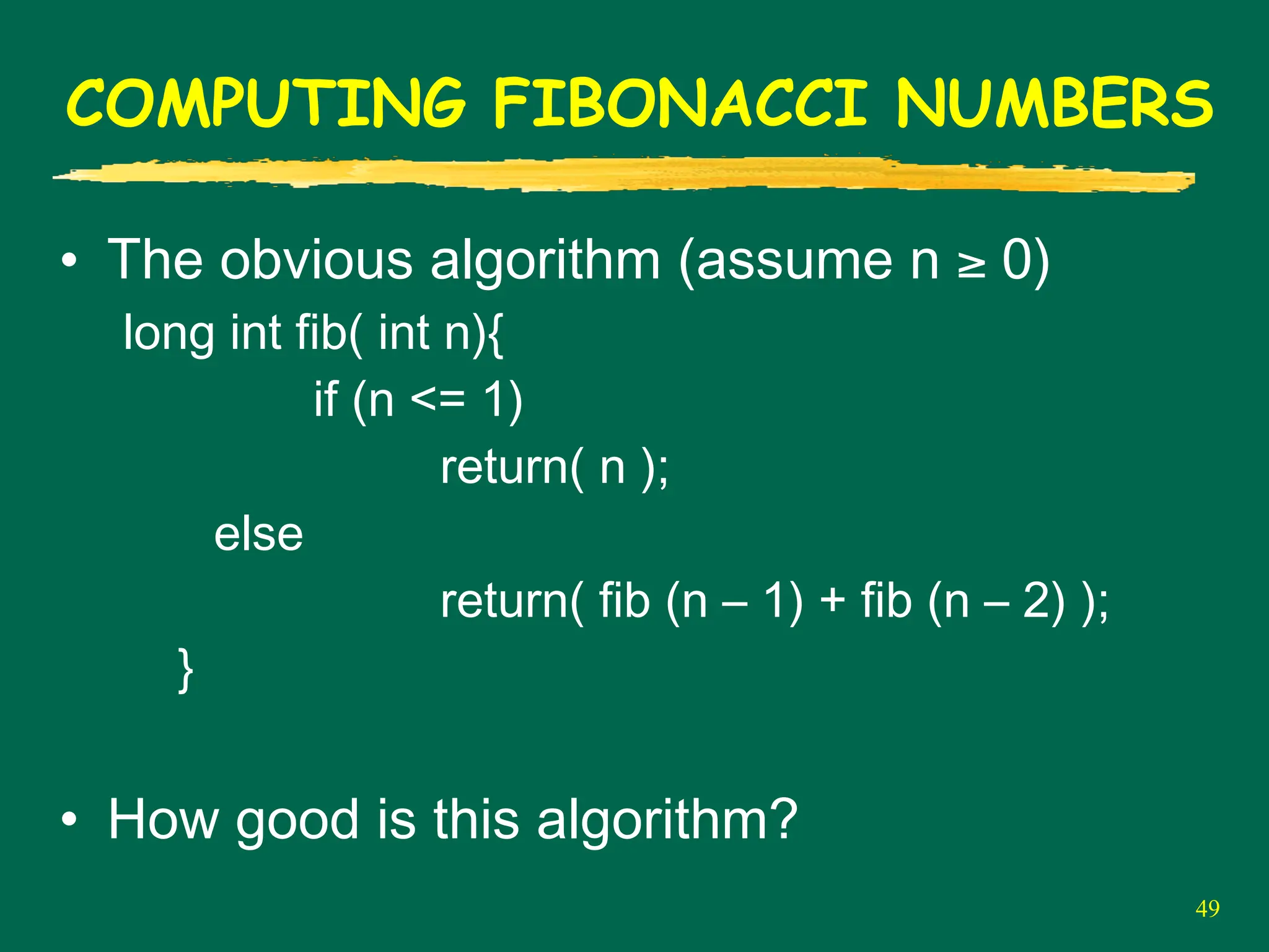
•The obvious algorithm (assume n ≥ 0)
long int fib( int n){
if (n <= 1)
return( n );
else
return( fib (n – 1) + fib (n – 2) );
}
• How good is this algorithm?
50.
50
COMPUTING FIBONACCI NUMBERS
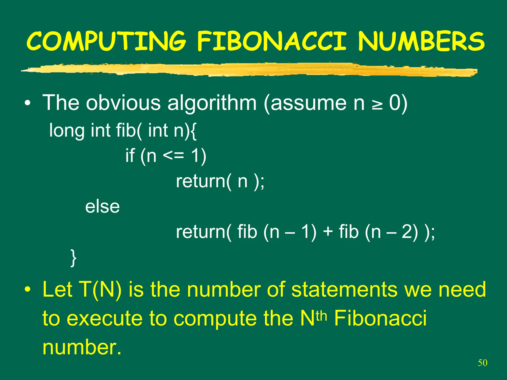
•The obvious algorithm (assume n ≥ 0)
long int fib( int n){
if (n <= 1)
return( n );
else
return( fib (n – 1) + fib (n – 2) );
}
• Let T(N) is the number of statements we need
to execute to compute the Nth Fibonacci
number.
51.
51
COMPUTING FIBONACCI NUMBERS
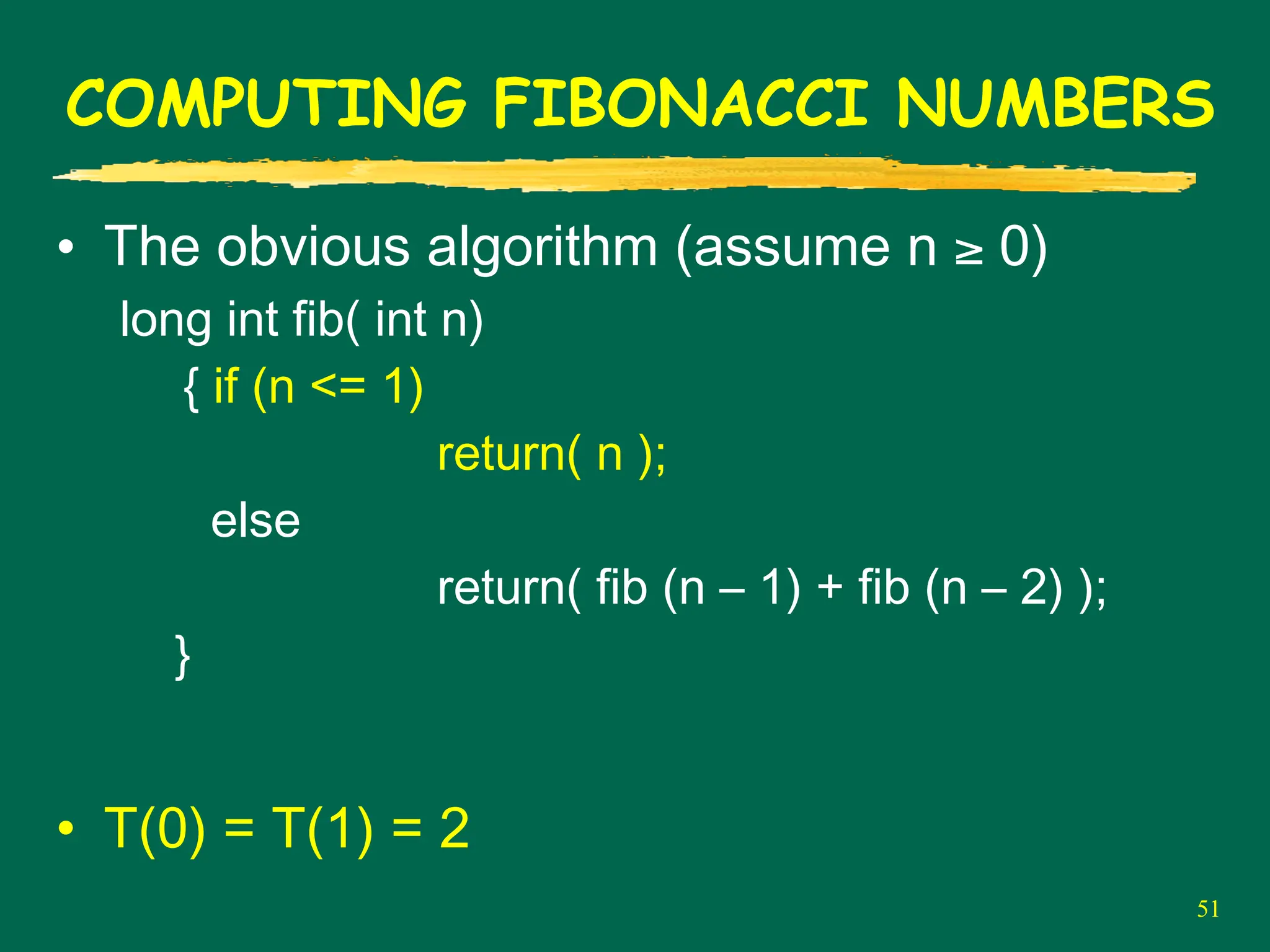
•The obvious algorithm (assume n ≥ 0)
long int fib( int n)
{ if (n <= 1)
return( n );
else
return( fib (n – 1) + fib (n – 2) );
}
• T(0) = T(1) = 2
52.
52
COMPUTING FIBONACCI NUMBERS
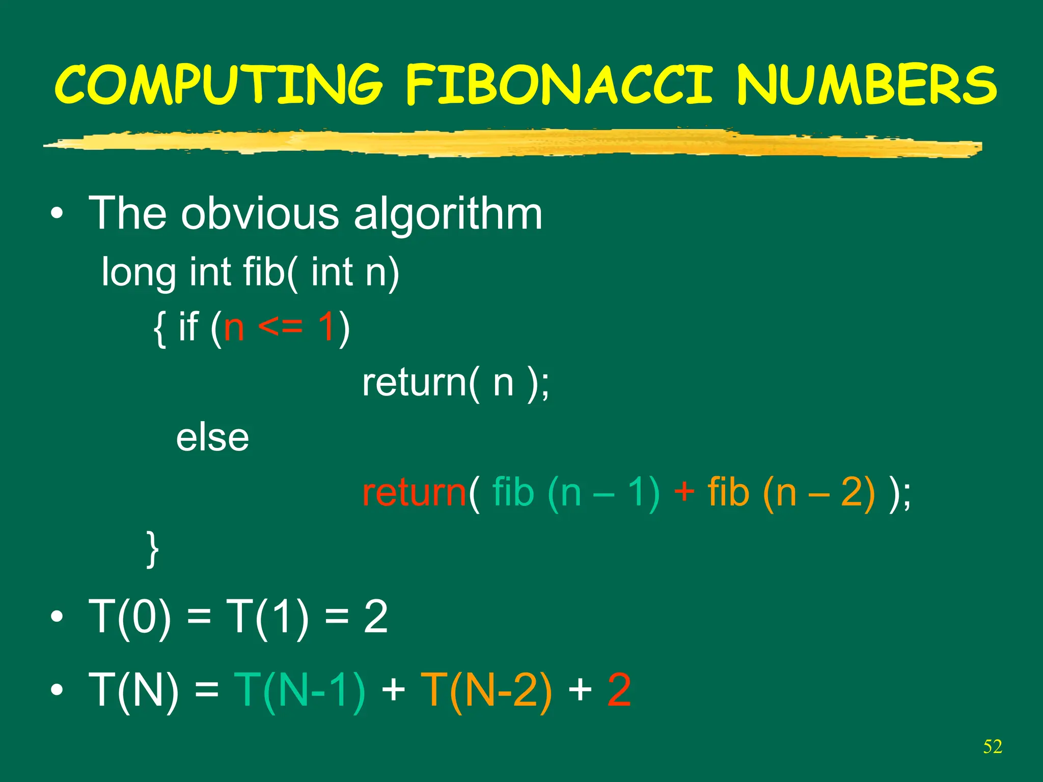
•The obvious algorithm
long int fib( int n)
{ if (n <= 1)
return( n );
else
return( fib (n – 1) + fib (n – 2) );
}
• T(0) = T(1) = 2
• T(N) = T(N-1) + T(N-2) + 2
53.
53
COMPUTING FIBONACCI NUMBERS
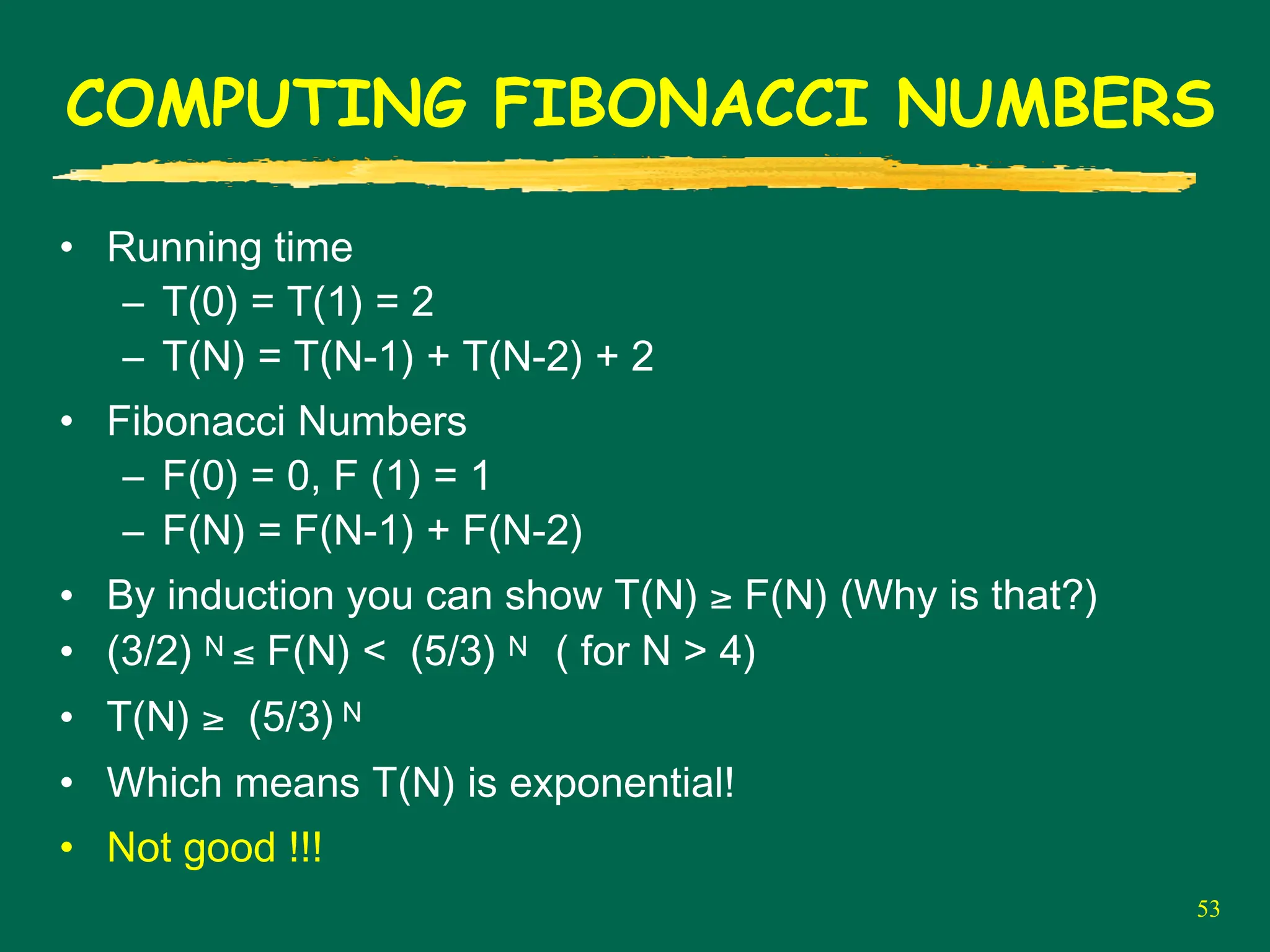
•Running time
– T(0) = T(1) = 2
– T(N) = T(N-1) + T(N-2) + 2
• Fibonacci Numbers
– F(0) = 0, F (1) = 1
– F(N) = F(N-1) + F(N-2)
• By induction you can show T(N) ≥ F(N) (Why is that?)
• (3/2) N ≤ F(N) < (5/3) N ( for N > 4)
• T(N) ≥ (5/3) N
• Which means T(N) is exponential!
• Not good !!!
56
COMPUTING FIBONACCI NUMBERS
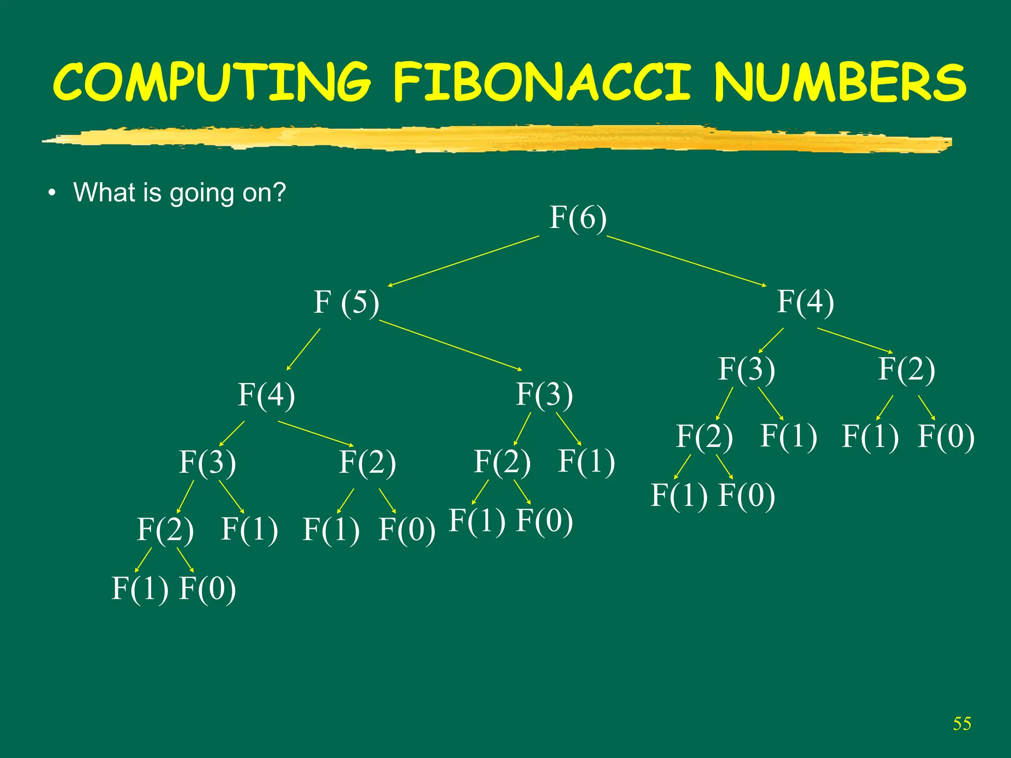
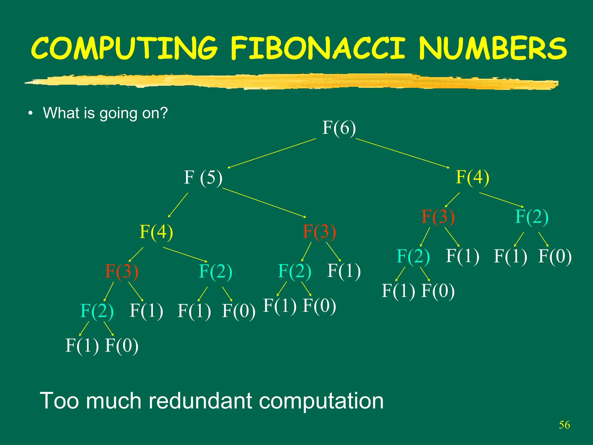
•What is going on?
F(6)
F (5)
F(4)
F(2)
F(1) F(0)
F(3)
F(2)
F(1) F(0)
F(1)
F(3)
F(2)
F(1) F(0)
F(1)
F(4)
F(2)
F(1) F(0)
F(3)
F(2)
F(1) F(0)
F(1)
Too much redundant computation
57.
57
COMPUTING FIBONACCI NUMBERS
•The next obvious algorithm (assume n ≥ 0)
int fib( int n)
{int X[3];
if (n <= 1) return(n);
X[0]=0; X[1]=1;
for (i = 2; i <= n; i++)
X[i % 3] = X[(i-1) % 3] + X[(i-2) % 3];
return X[(i-1)%3] ;
}
58.
58
COMPUTING FIBONACCI NUMBERS
•The next obvious algorithm (assume n ≥ 0)
int fib( int n)
{int X[3];
if (n <= 1) return(n);
X[0]=0; X[1]=1;
for (i = 2; i <= n; i++)
X[i % 3] = X[(i-1) % 3] + X[(i-2) % 3];
return X[(i-1)%3] ;
}
• % is the mod operator i%3 ≡ i mod 3
59.
59
COMPUTING FIBONACCI NUMBERS
•The next obvious algorithm (assume n ≥ 0)
int fib( int n)
{int X[3];
if (n <= 1) return(n);
X[0]=0; X[1]=1;
for (i = 2; i <= n; i++)
X[i % 3] = X[(i-1) % 3] + X[(i-2) % 3];
return X[(i-1)%3] ;
}
0
1
X[0]
X[1]
X[2]
when i=2
fib(0)
fib(1)
60.
60
COMPUTING FIBONACCI NUMBERS
•The next obvious algorithm (assume n ≥ 0)
int fib( int n)
{int X[3];
if (n <= 1) return(n);
X[0]=0; X[1]=1;
for (i = 2; i <= n; i++)
X[i % 3] = X[(i-1) % 3] + X[(i-2) % 3];
return X[(i-1)%3] ;
}
0
1
1
X[0]
X[1]
X[2]
fib(2) fib(1)
fib(0)
61.
61
COMPUTING FIBONACCI NUMBERS
•The next obvious algorithm (assume n ≥ 0)
int fib( int n)
{int X[3];
if (n <= 1) return(n);
X[0]=0; X[1]=1;
for (i = 2; i <= n; i++)
X[i % 3] = X[(i-1) % 3] + X[(i-2) % 3];
return X[(i-1)%3] ;
}
2
1
1
X[0]
X[1]
X[2]
fib(3)
fib(2) fib(1)
62.
62
COMPUTING FIBONACCI NUMBERS
•The next obvious algorithm (assume n ≥ 0)
int fib( int n)
{int X[3];
if (n <= 1) return(n);
X[0]=0; X[1]=1;
for (i = 2; i <= n; i++)
X[i % 3] = X[(i-1) % 3] + X[(i-2) % 3];
return X[(i-1)%3] ;
}
2
3
1
X[0]
X[1]
X[2]
fib(4)
fib(3)
fib(2)
63.
63
COMPUTING FIBONACCI NUMBERS
•The next obvious algorithm (assume n ≥ 0)
int fib( int n)
{int X[3];
if (n <= 1) return(n);
X[0]=0; X[1]=1;
for (i = 2; i <= n; i++)
X[i % 3] = X[(i-1) % 3] + X[(i-2) % 3];
return X[(i-1)%3] ;
}
2
3
5
X[0]
X[1]
X[2]
fib(5)
64.
64
COMPUTING FIBONACCI NUMBERS
•The next obvious algorithm (assume n ≥ 0)
int fib( int n)
{int X[3];
if (n <= 1) return(n);
X[0]=0; X[1]=1;
for (i = 2; i <= n; i++)
X[i % 3] = X[(i-1) % 3] + X[(i-2) % 3];
return X[(i-1)%3] ; (Why?)
}
• Because i is incremented at the end of the loop
before exit.
65.
65
COMPUTING FIBONACCI NUMBERS
•The next obvious algorithm (assume n ≥ 0)
int fib( int n)
{int X[3];
if (n <= 1) return(n);
X[0]=0; X[1]=1;
for (i = 2; i <= n; i++)
X[i % 3] = X[(i-1) % 3] + X[(i-2) % 3];
return X[(i-1)%3] ;
}
• ~N iterations each taking constant time → O(N)
66.
66
COMPUTING FIBONACCI NUMBERS
•The next obvious algorithm (assume n ≥ 0)
int fib( int n)
{int X[3];
if (n <= 1) return(n);
X[0]=0; X[1]=1;
for (i = 2; i <= n; i++)
X[i % 3] = X[(i-1) % 3] + X[(i-2) % 3];
return X[(i-1)%3] ;
}
• ~N iterations each taking constant time → O(N)
• Much better than the O(cN) algorithm, but ....
69
COMPUTING FIBONACCI NUMBERS
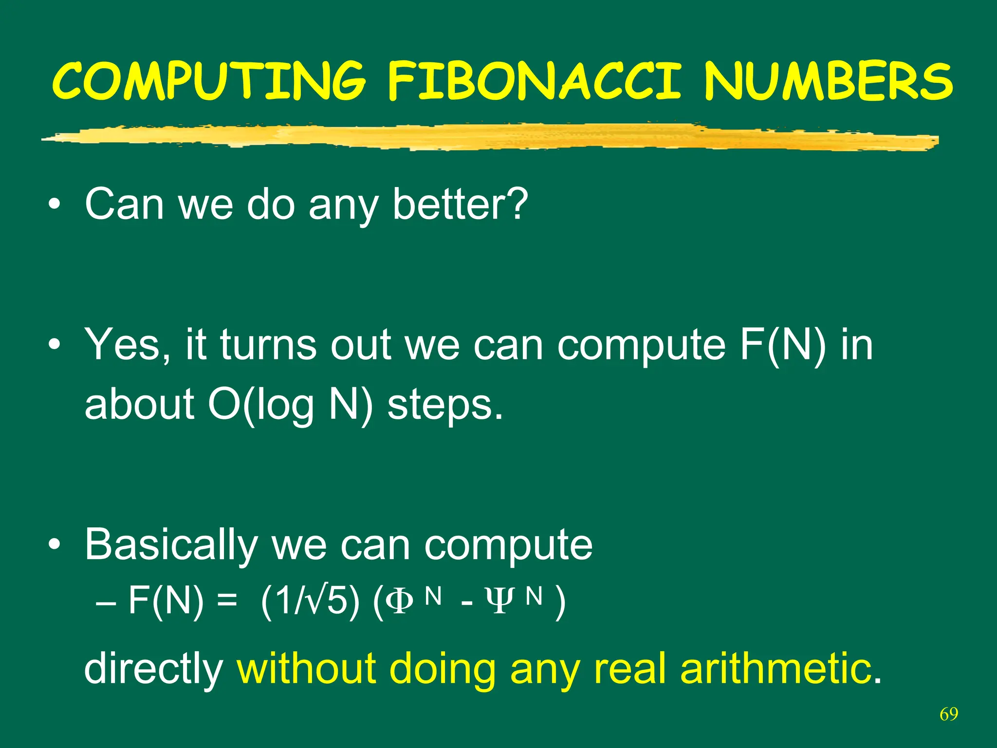
•Can we do any better?
• Yes, it turns out we can compute F(N) in
about O(log N) steps.
• Basically we can compute
– F(N) = (1/√5) (Φ N - Ψ N )
directly without doing any real arithmetic.
73
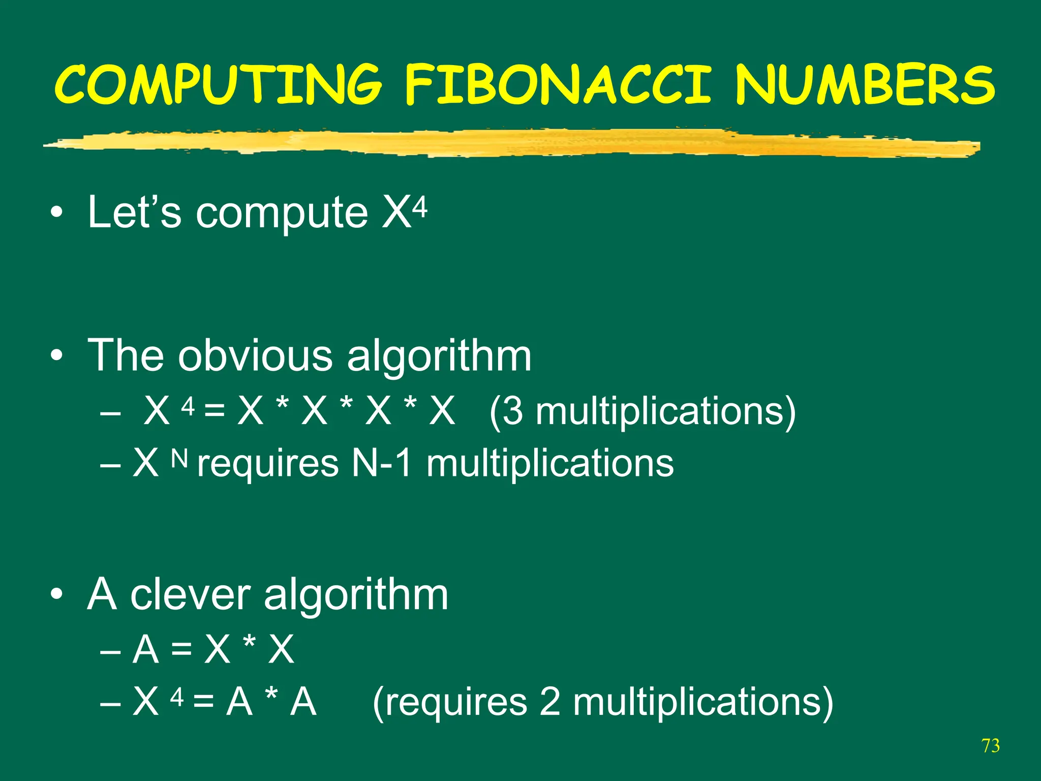
COMPUTING FIBONACCI NUMBERS
•Let’s compute X4
• The obvious algorithm
– X 4 = X * X * X * X (3 multiplications)
– X N requires N-1 multiplications
• A clever algorithm
– A = X * X
– X 4 = A * A (requires 2 multiplications)
74.
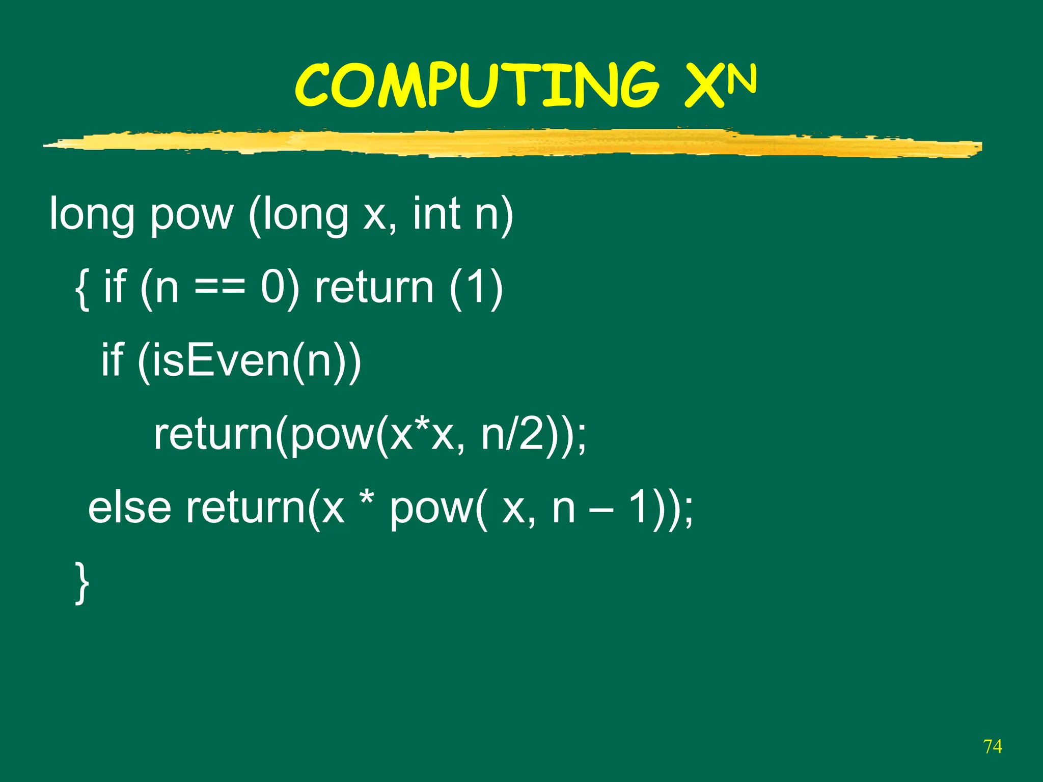
74
COMPUTING XN
long pow(long x, int n)
{ if (n == 0) return (1)
if (isEven(n))
return(pow(x*x, n/2));
else return(x * pow( x, n – 1));
}
75.
75
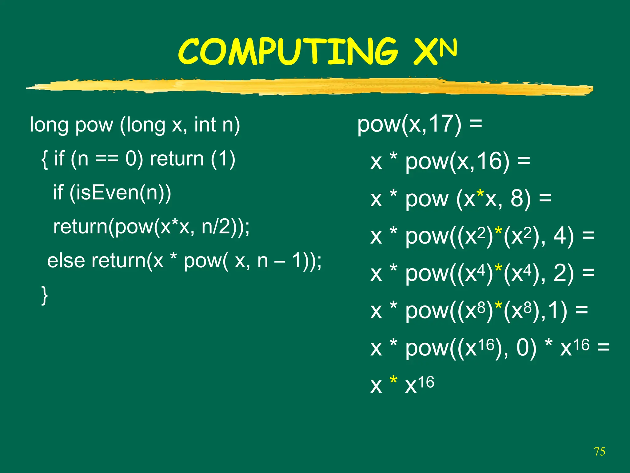
COMPUTING XN
long pow(long x, int n)
{ if (n == 0) return (1)
if (isEven(n))
return(pow(x*x, n/2));
else return(x * pow( x, n – 1));
}
pow(x,17) =
x * pow(x,16) =
x * pow (x*x, 8) =
x * pow((x2)*(x2), 4) =
x * pow((x4)*(x4), 2) =
x * pow((x8)*(x8),1) =
x * pow((x16), 0) * x16 =
x * x16
76.
76
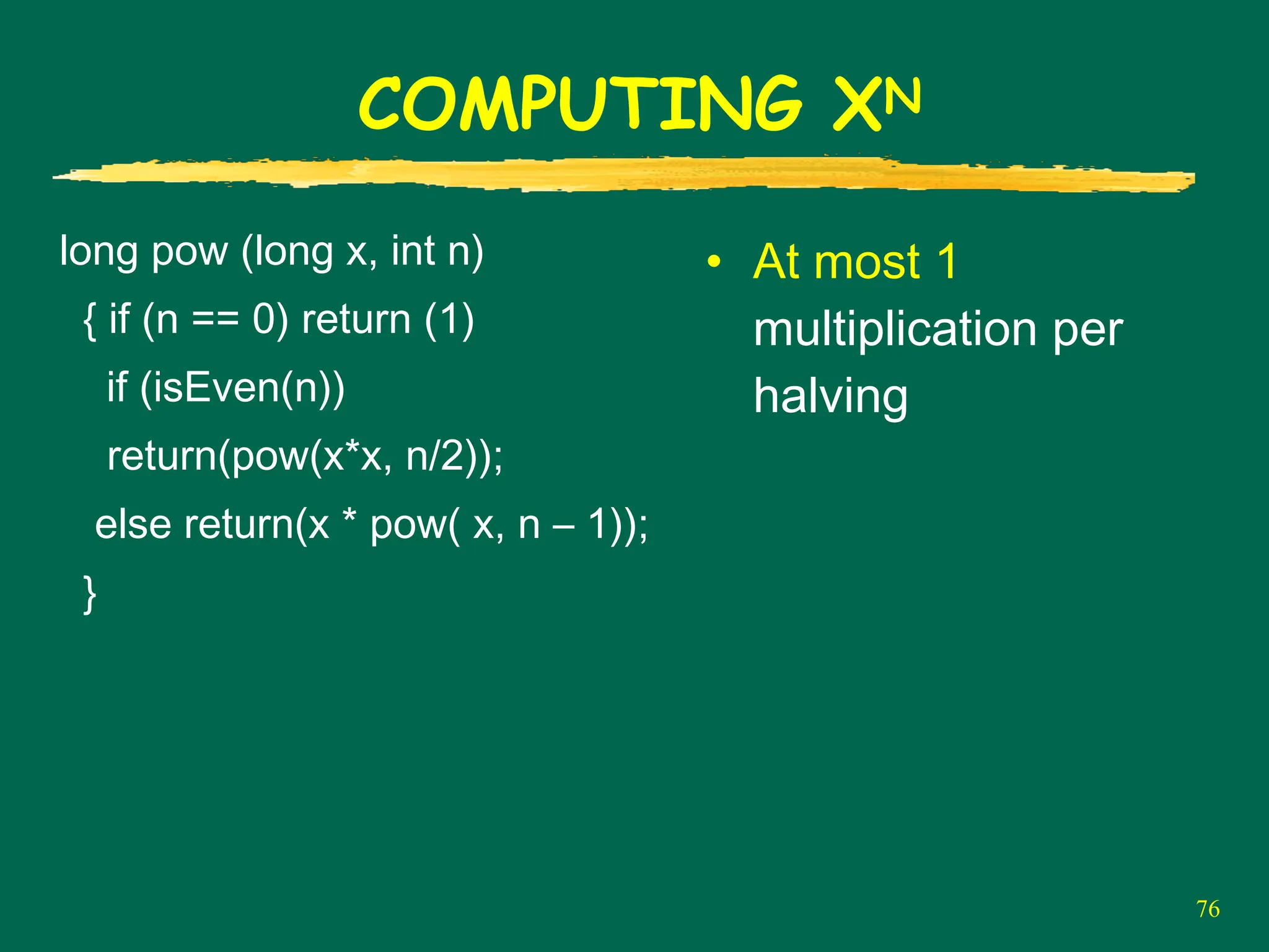
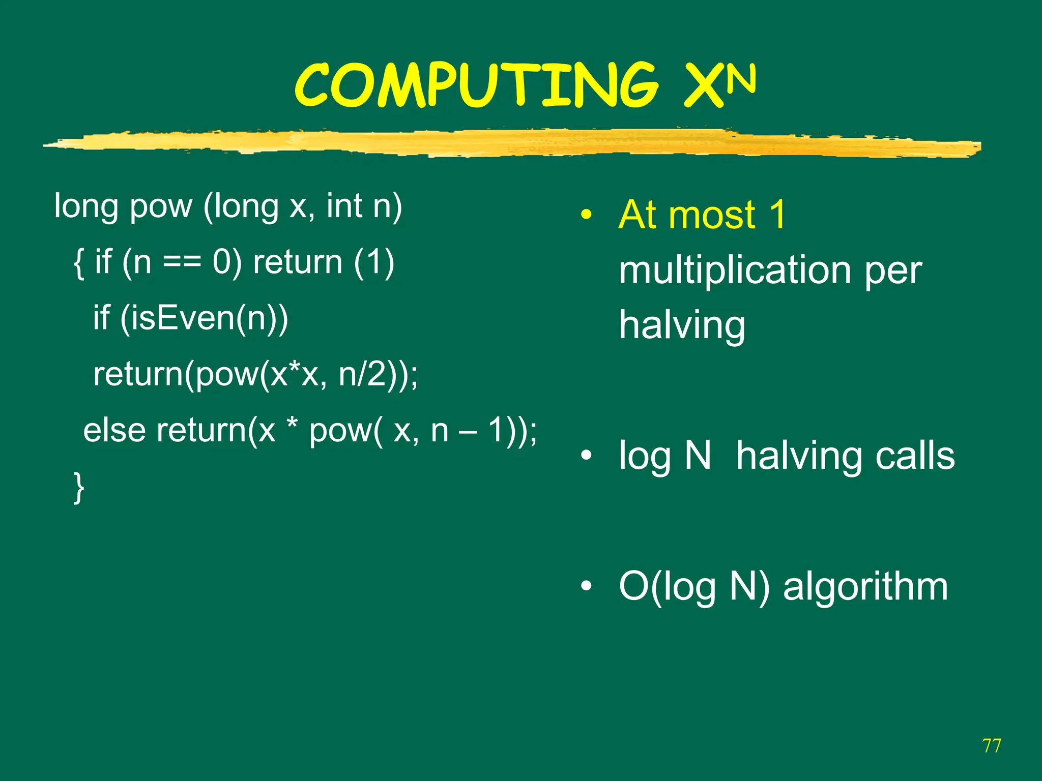
COMPUTING XN
long pow(long x, int n)
{ if (n == 0) return (1)
if (isEven(n))
return(pow(x*x, n/2));
else return(x * pow( x, n – 1));
}
• At most 1
multiplication per
halving
77.
77
COMPUTING XN
long pow(long x, int n)
{ if (n == 0) return (1)
if (isEven(n))
return(pow(x*x, n/2));
else return(x * pow( x, n – 1));
}
• At most 1
multiplication per
halving
• log N halving calls
• O(log N) algorithm
78.
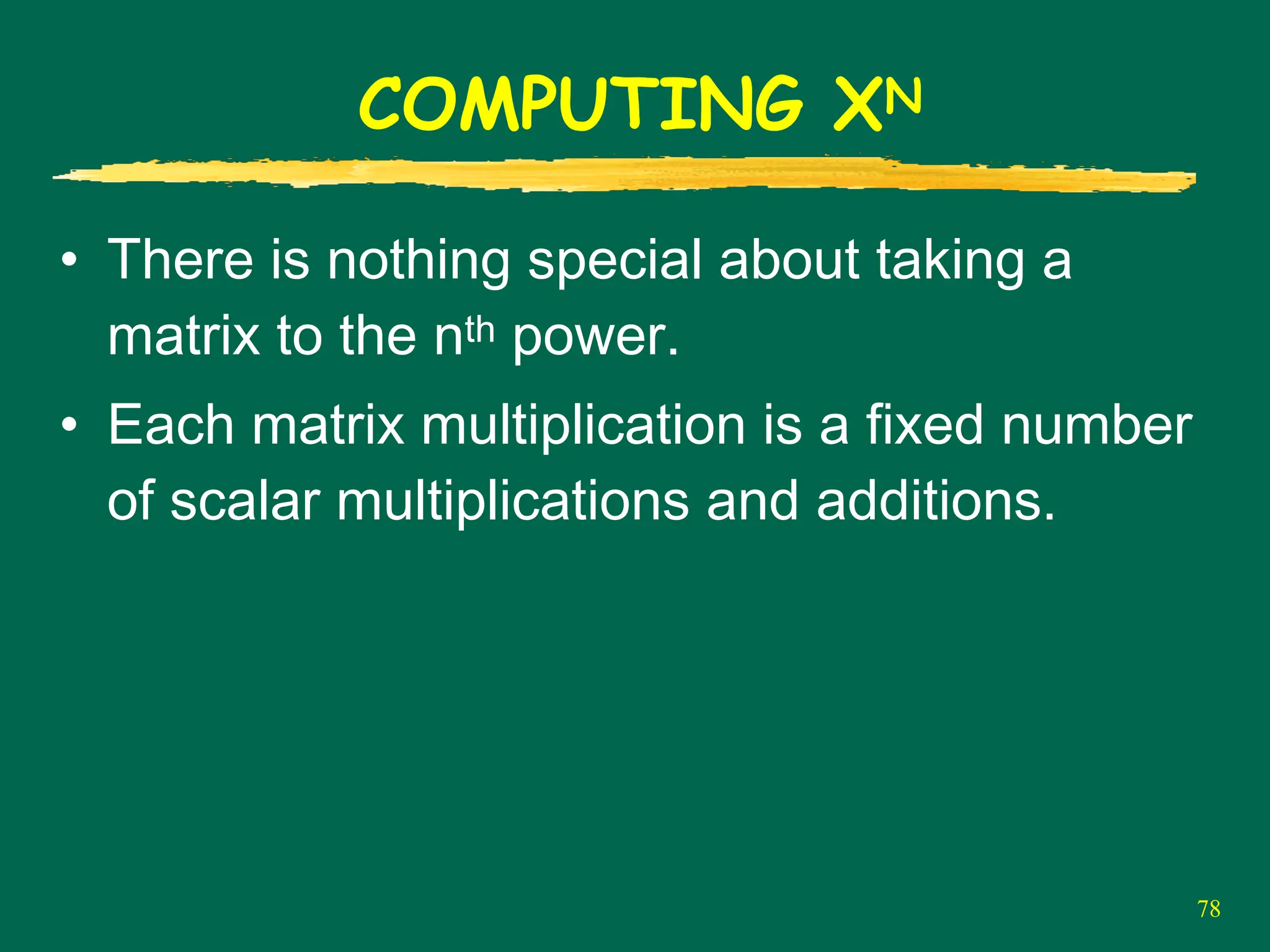
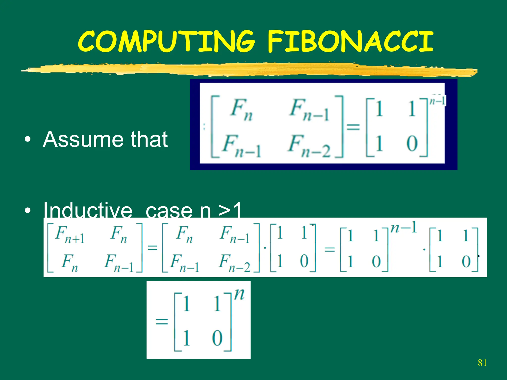
COMPUTING XN
• Thereis nothing special about taking a
matrix to the nth power.
• Each matrix multiplication is a fixed number
of scalar multiplications and additions.
78
82
PROBLEMS, ALGORITHMS ANDBOUNDS
• To show a problem is O(f(N)): demonstrate
a correct algorithm which solves the
problem and takes O(f(N)) time.
83.
83
PROBLEMS, ALGORITHMS ANDBOUNDS
• To show a problem is O(f(N)): demonstrate a
correct algorithm which solves the problem
and takes O(f(N)) time. (Usually easy!)
• To show a problem is Ω(f(N)): Show that ALL
algorithms solving the problem must take at
least Ω(f(N)) time. (Usually very hard!)
84.
84
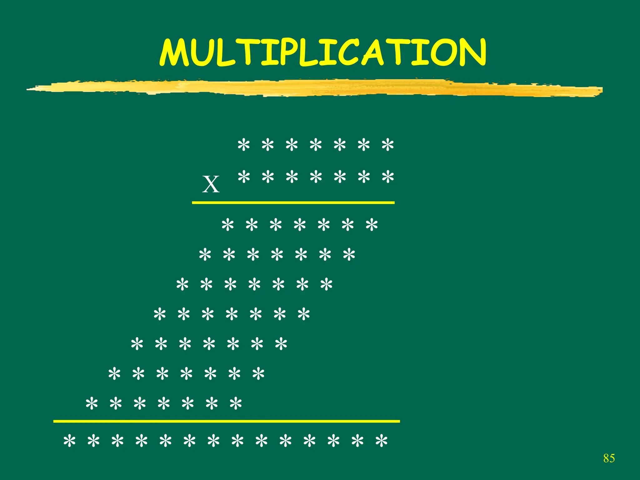
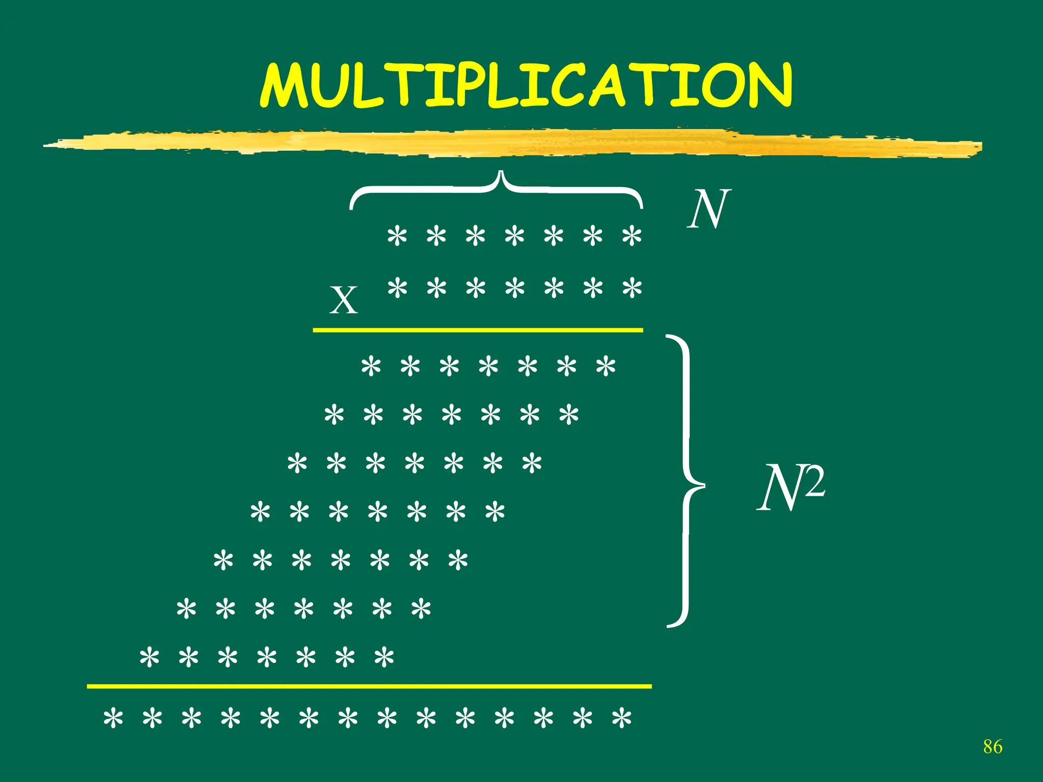
(Back to) MULTIPLICATION
•Elementary school addition : Θ(N)
– We have an algorithm which runs in O(N) time
– We need at least Ω(N) time
• Elementary school multiplication: O(N2)
– We have an algorithm which runs in O(N2) time.
87
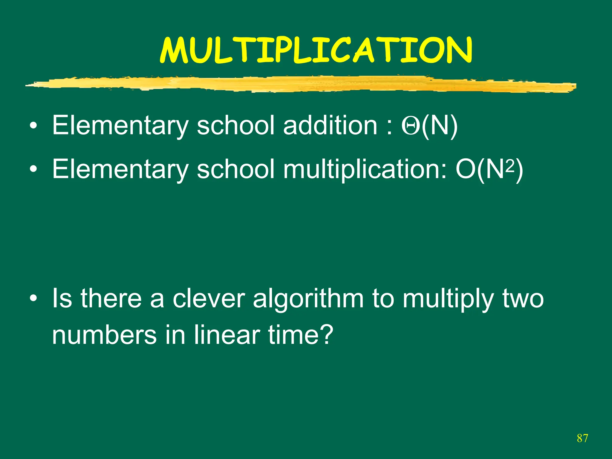
MULTIPLICATION
• Elementary schooladdition : Θ(N)
• Elementary school multiplication: O(N2)
• Is there a clever algorithm to multiply two
numbers in linear time?
88.
88
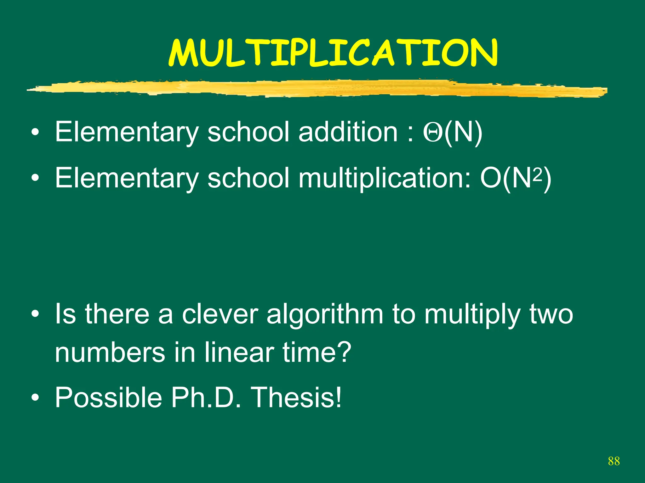
MULTIPLICATION
• Elementary schooladdition : Θ(N)
• Elementary school multiplication: O(N2)
• Is there a clever algorithm to multiply two
numbers in linear time?
• Possible Ph.D. Thesis!
89.
89
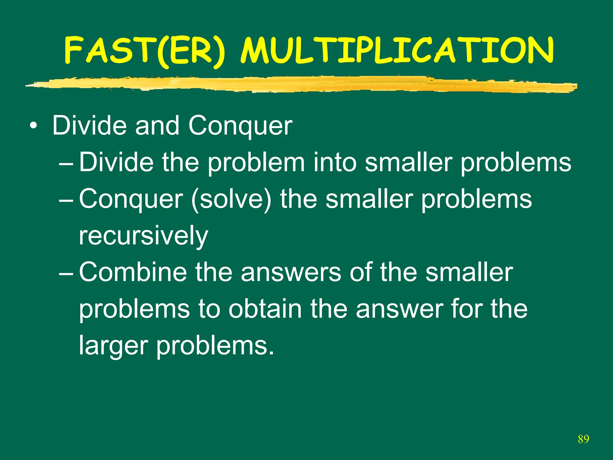
FAST(ER) MULTIPLICATION
• Divideand Conquer
– Divide the problem into smaller problems
– Conquer (solve) the smaller problems
recursively
– Combine the answers of the smaller
problems to obtain the answer for the
larger problems.
90.
90
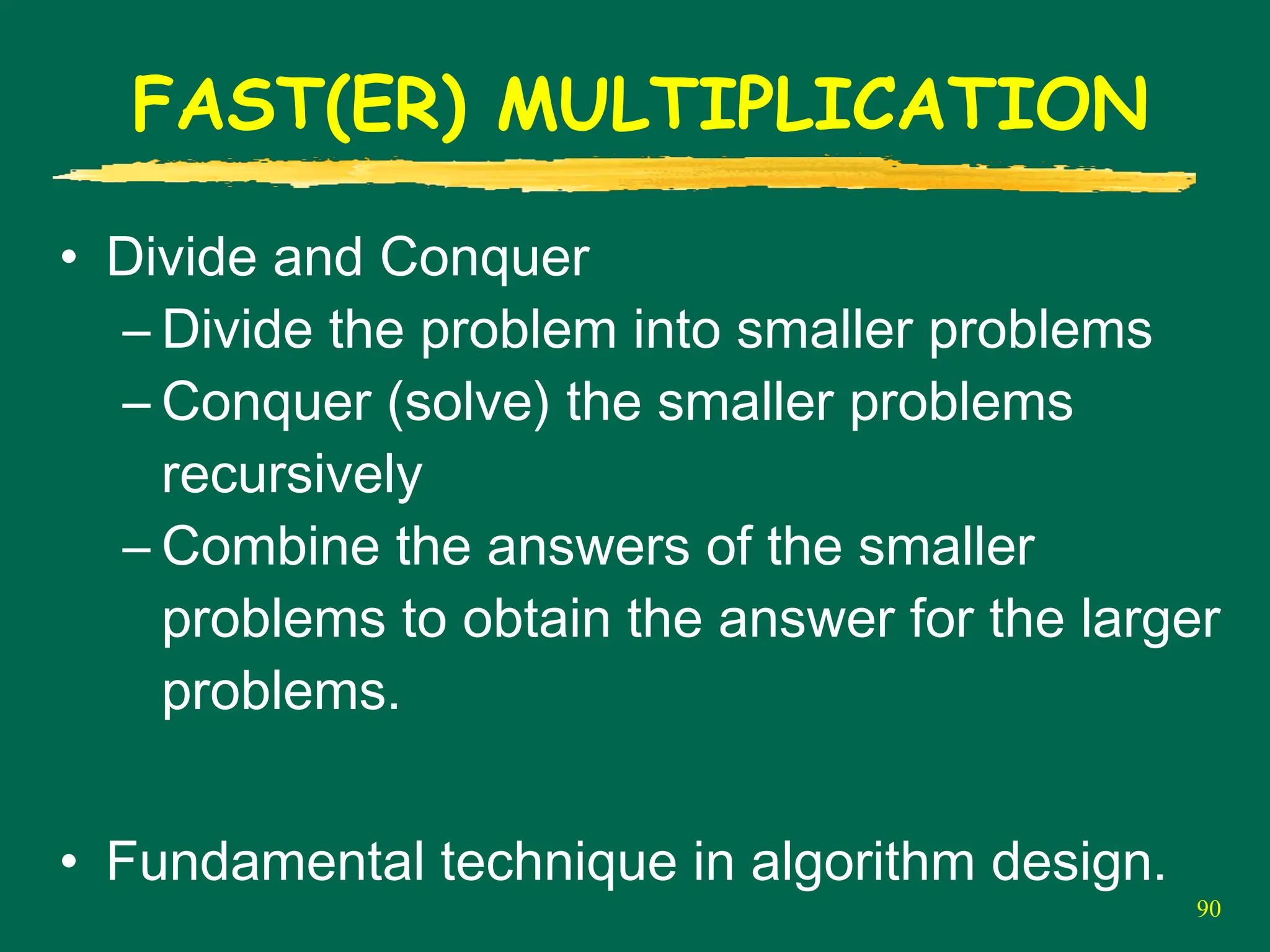
FAST(ER) MULTIPLICATION
• Divideand Conquer
– Divide the problem into smaller problems
– Conquer (solve) the smaller problems
recursively
– Combine the answers of the smaller
problems to obtain the answer for the larger
problems.
• Fundamental technique in algorithm design.
95
SHIFTS
• Multiply by2 is the same as shift left by 1
bit.
• Just as Multiply by 10 is the same as shift
left by 1 digit
– 40 * 10 = 400
96.
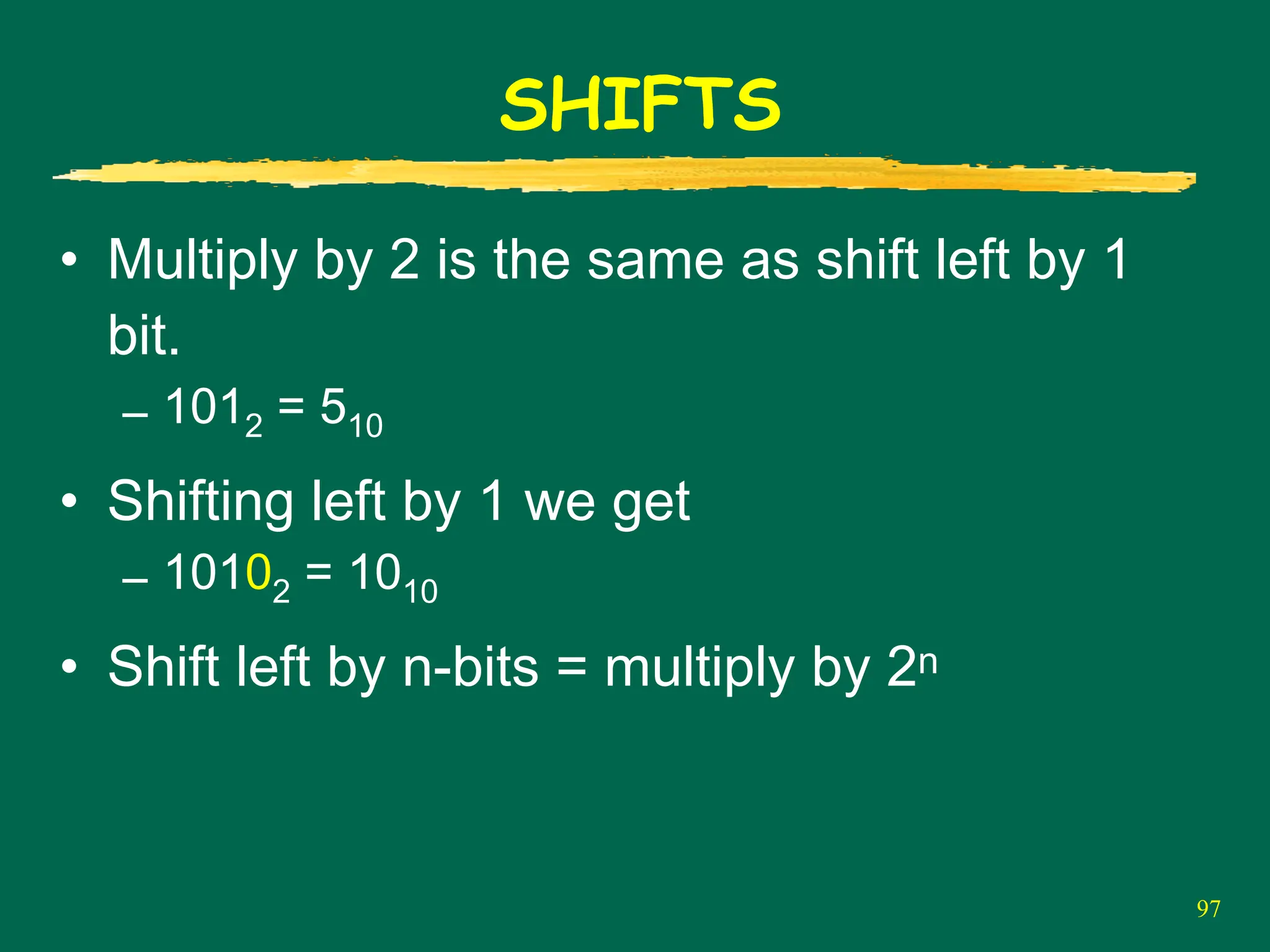
96
SHIFTS
• Multiply by2 is the same as shift left by 1
bit.
– 1012 = 510
• Shifting left by 1 we get
– 10102 = 1010
97.
97
SHIFTS
• Multiply by2 is the same as shift left by 1
bit.
– 1012 = 510
• Shifting left by 1 we get
– 10102 = 1010
• Shift left by n-bits = multiply by 2n
98.
98
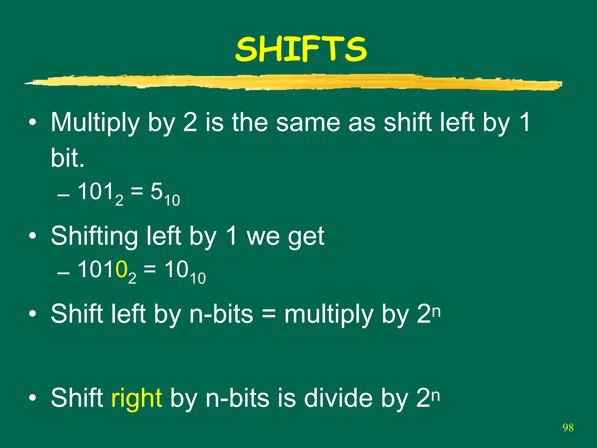
SHIFTS
• Multiply by2 is the same as shift left by 1
bit.
– 1012 = 510
• Shifting left by 1 we get
– 10102 = 1010
• Shift left by n-bits = multiply by 2n
• Shift right by n-bits is divide by 2n
99.
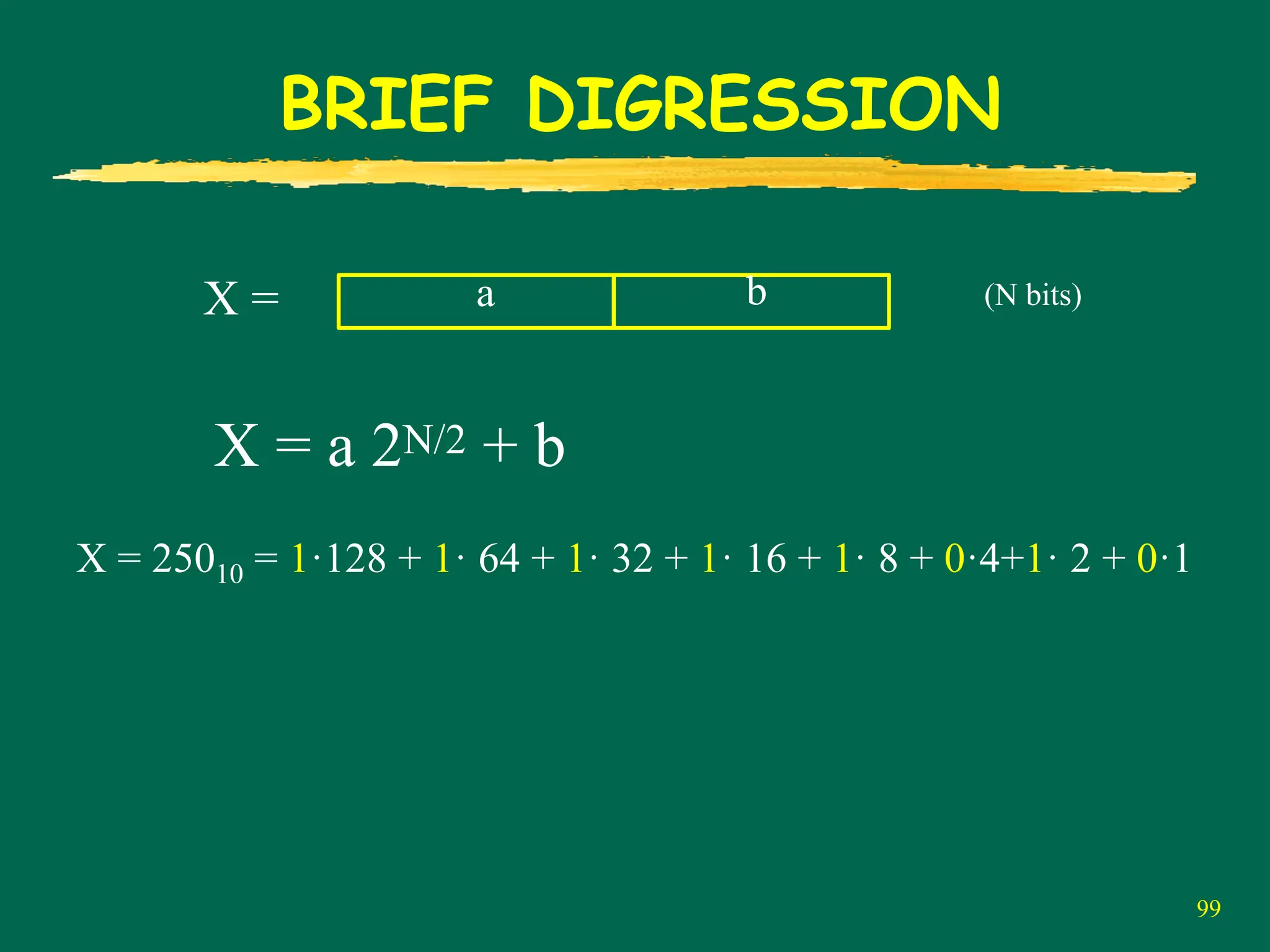
99
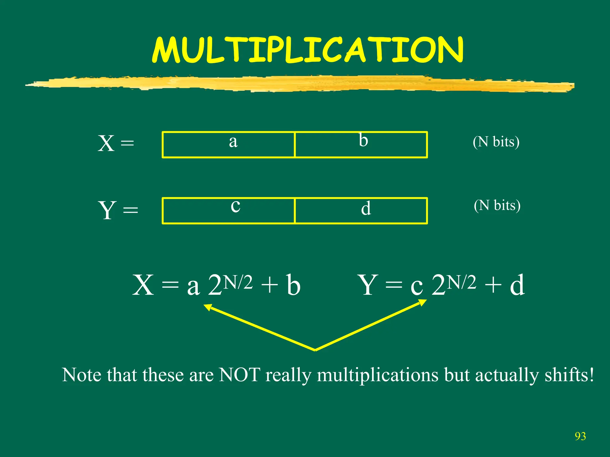
BRIEF DIGRESSION
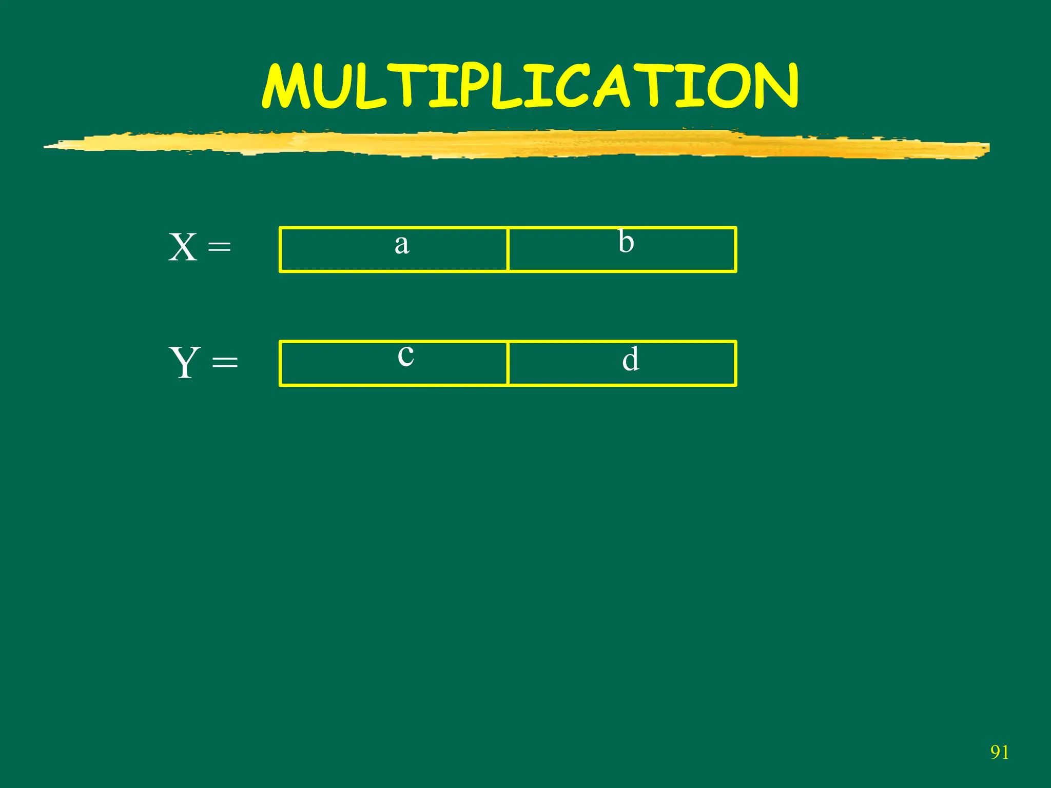
X =a b
X = a 2N/2 + b
(N bits)
X = 25010 = 1·128 + 1· 64 + 1· 32 + 1· 16 + 1· 8 + 0·4+1· 2 + 0·1
100.
100
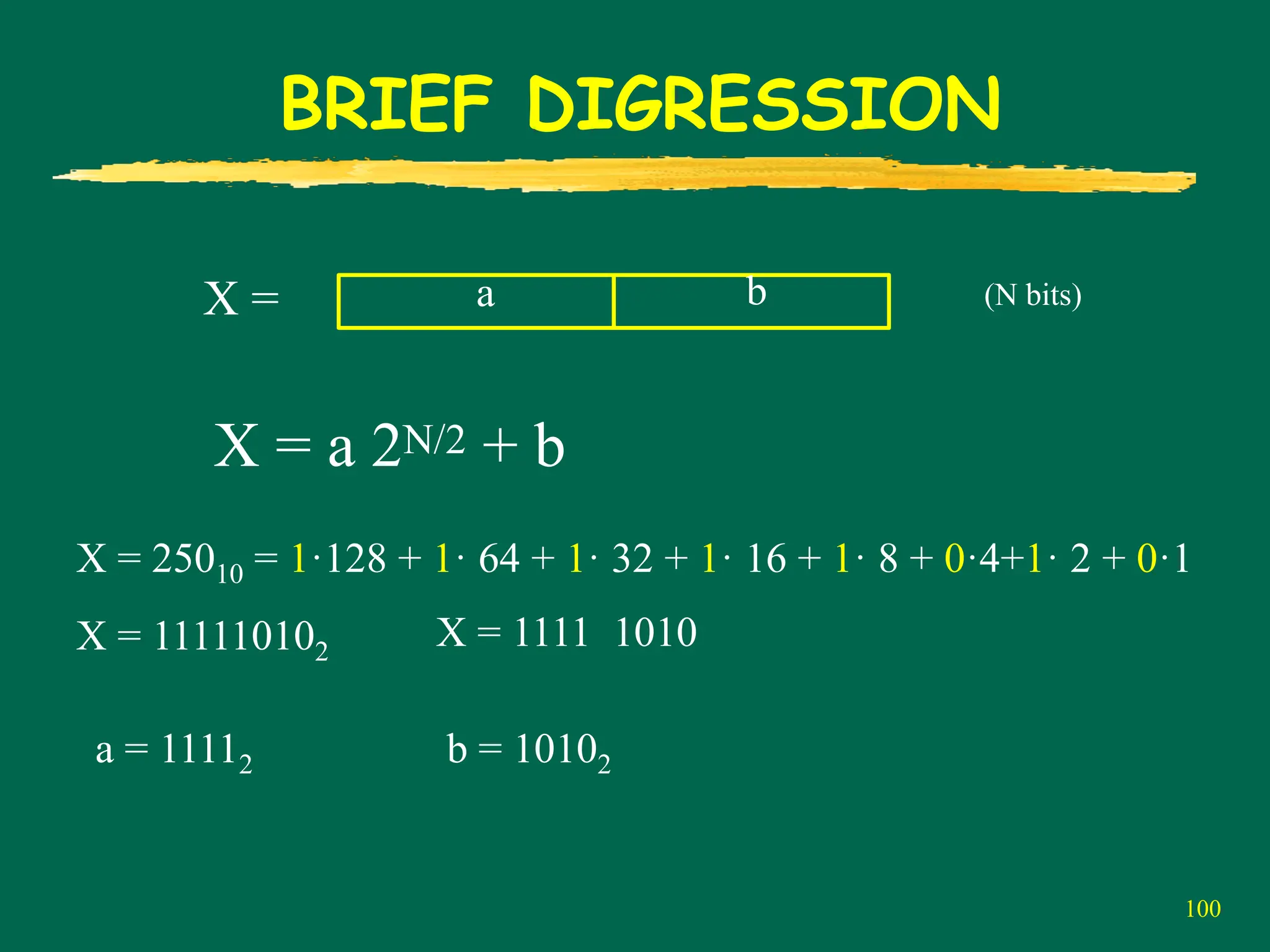
BRIEF DIGRESSION
X =a b
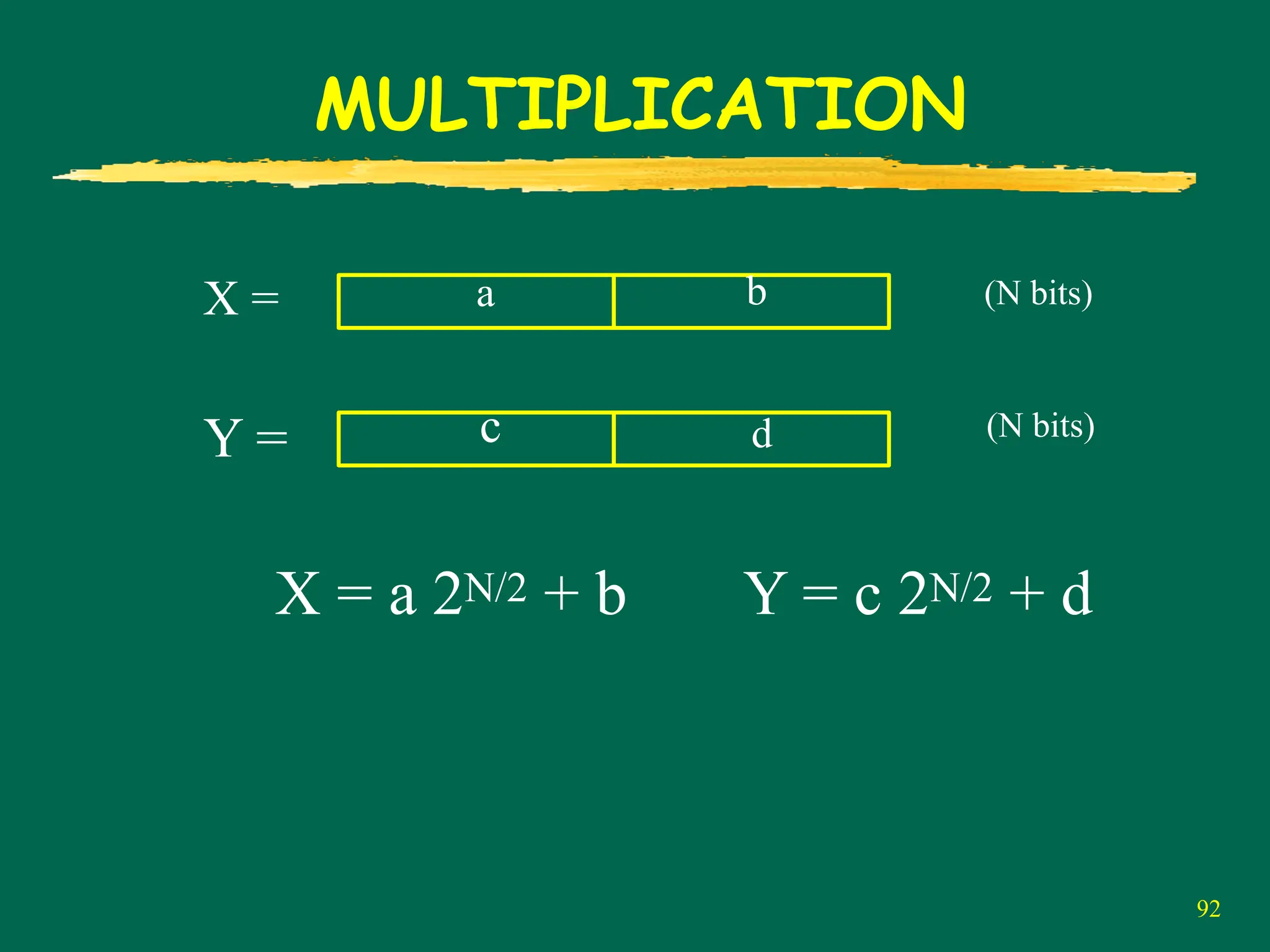
X = a 2N/2 + b
(N bits)
X = 25010 = 1·128 + 1· 64 + 1· 32 + 1· 16 + 1· 8 + 0·4+1· 2 + 0·1
X = 111110102
X = 1111 1010
a = 11112 b = 10102
101.
101
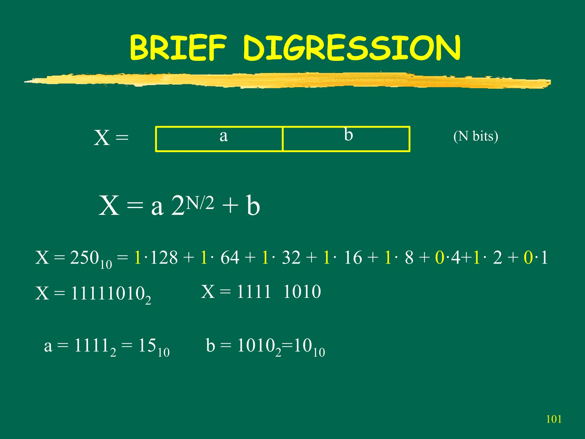
BRIEF DIGRESSION
X =a b
X = a 2N/2 + b
(N bits)
X = 25010 = 1·128 + 1· 64 + 1· 32 + 1· 16 + 1· 8 + 0·4+1· 2 + 0·1
X = 111110102
X = 1111 1010
a = 11112 = 1510 b = 10102=1010
102.
102
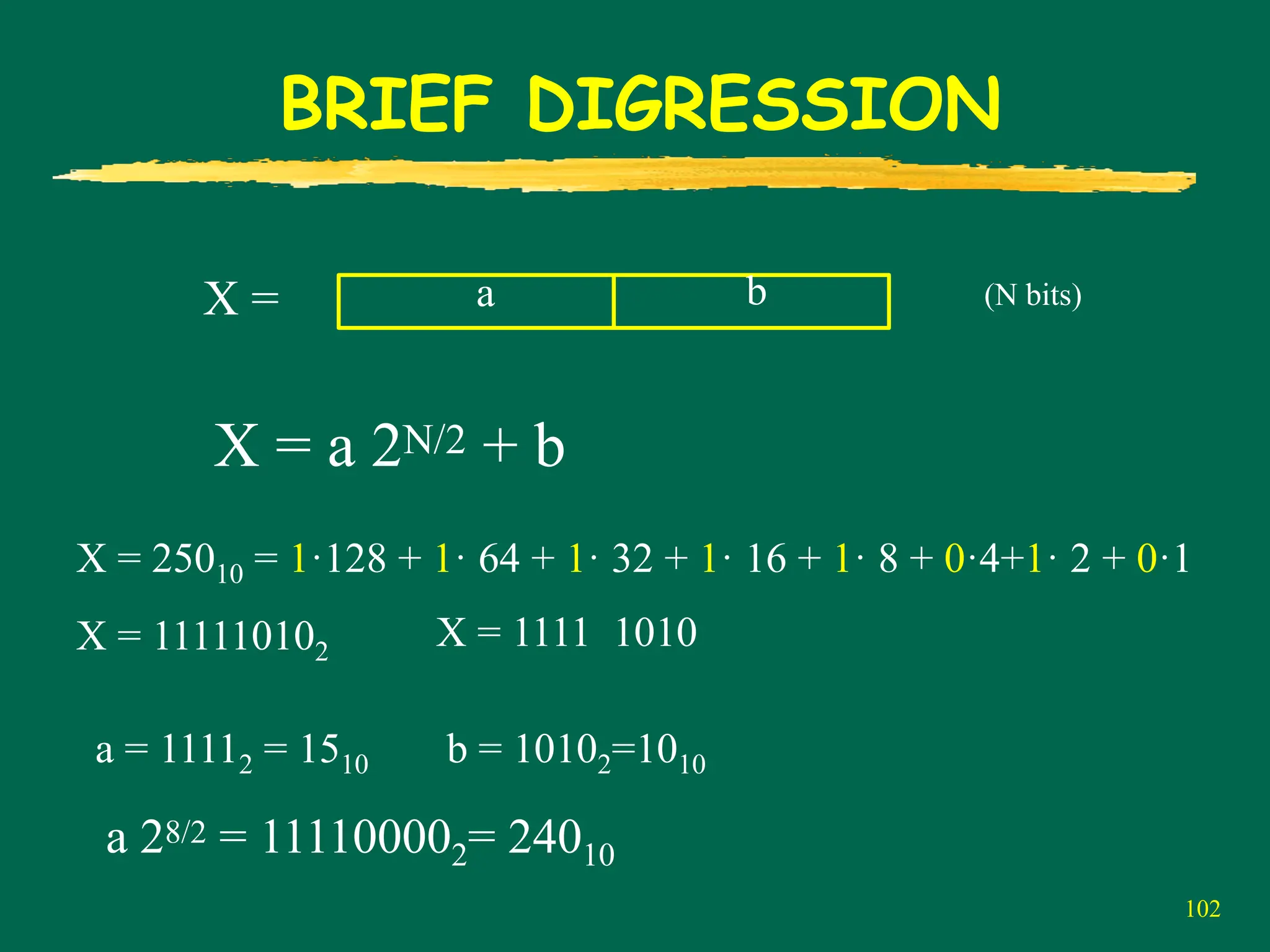
BRIEF DIGRESSION
X =a b
X = a 2N/2 + b
(N bits)
X = 25010 = 1·128 + 1· 64 + 1· 32 + 1· 16 + 1· 8 + 0·4+1· 2 + 0·1
X = 111110102
X = 1111 1010
a = 11112 = 1510 b = 10102=1010
a 28/2 = 111100002= 24010
103.
103
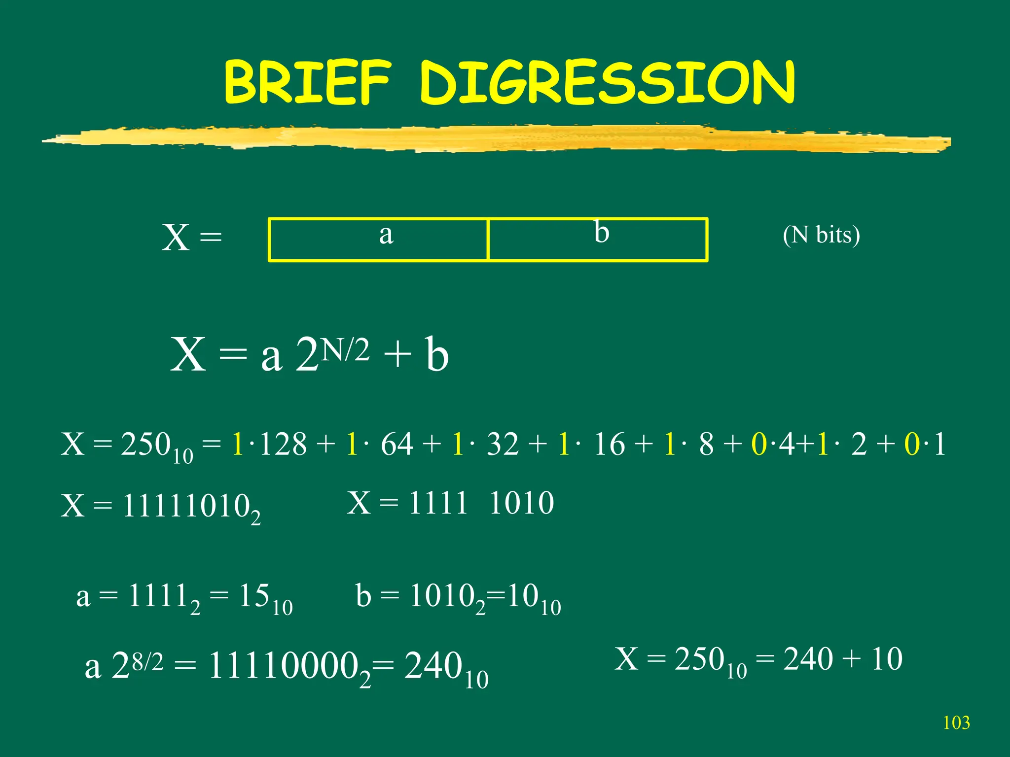
BRIEF DIGRESSION
X =a b
X = a 2N/2 + b
(N bits)
X = 25010 = 1·128 + 1· 64 + 1· 32 + 1· 16 + 1· 8 + 0·4+1· 2 + 0·1
X = 111110102
X = 1111 1010
a = 11112 = 1510 b = 10102=1010
a 28/2 = 111100002= 24010
X = 25010 = 240 + 10
104.
104
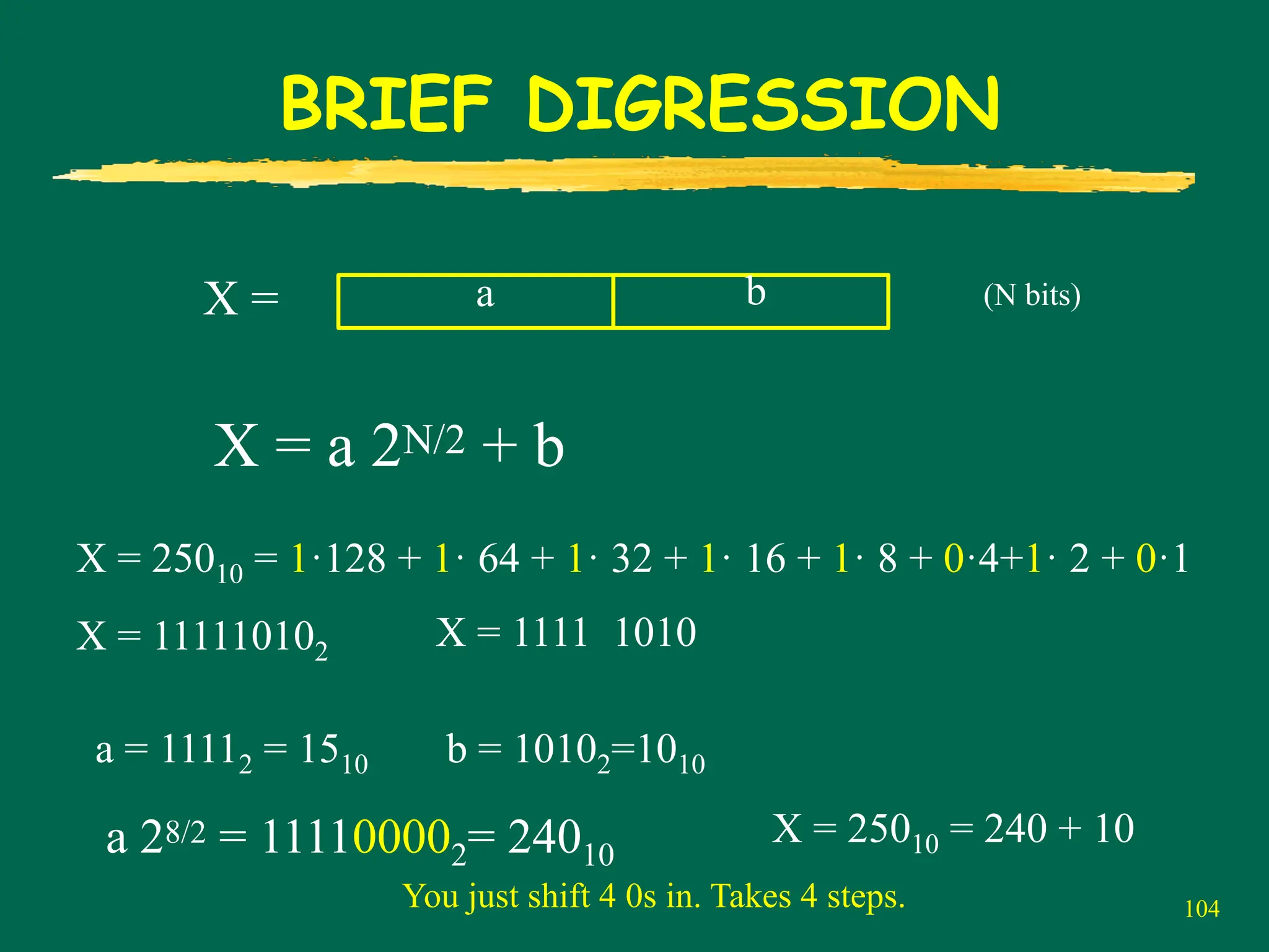
BRIEF DIGRESSION
X =a b
X = a 2N/2 + b
(N bits)
X = 25010 = 1·128 + 1· 64 + 1· 32 + 1· 16 + 1· 8 + 0·4+1· 2 + 0·1
X = 111110102
X = 1111 1010
a = 11112 = 1510 b = 10102=1010
a 28/2 = 111100002= 24010
X = 25010 = 240 + 10
You just shift 4 0s in. Takes 4 steps.
106
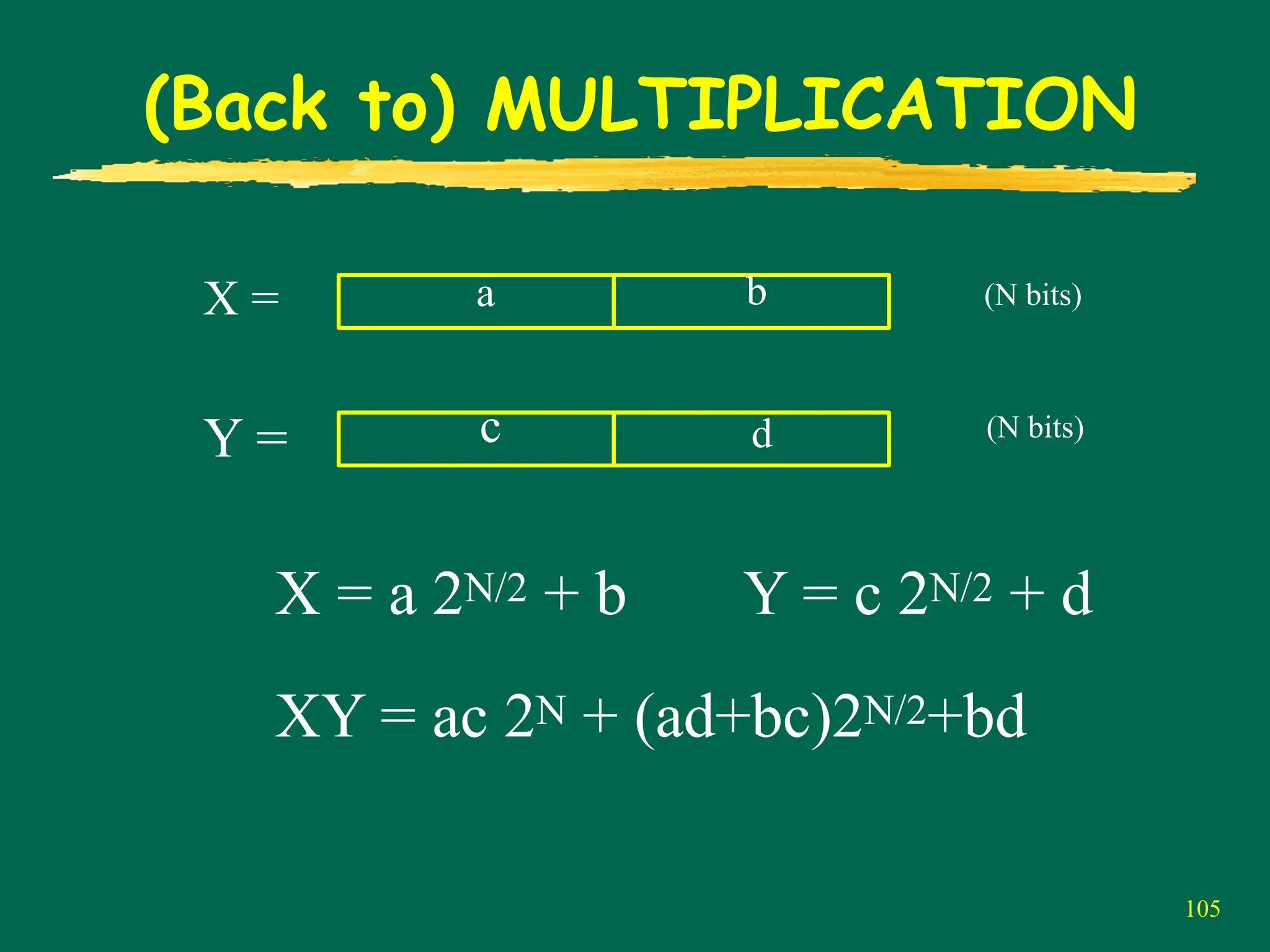
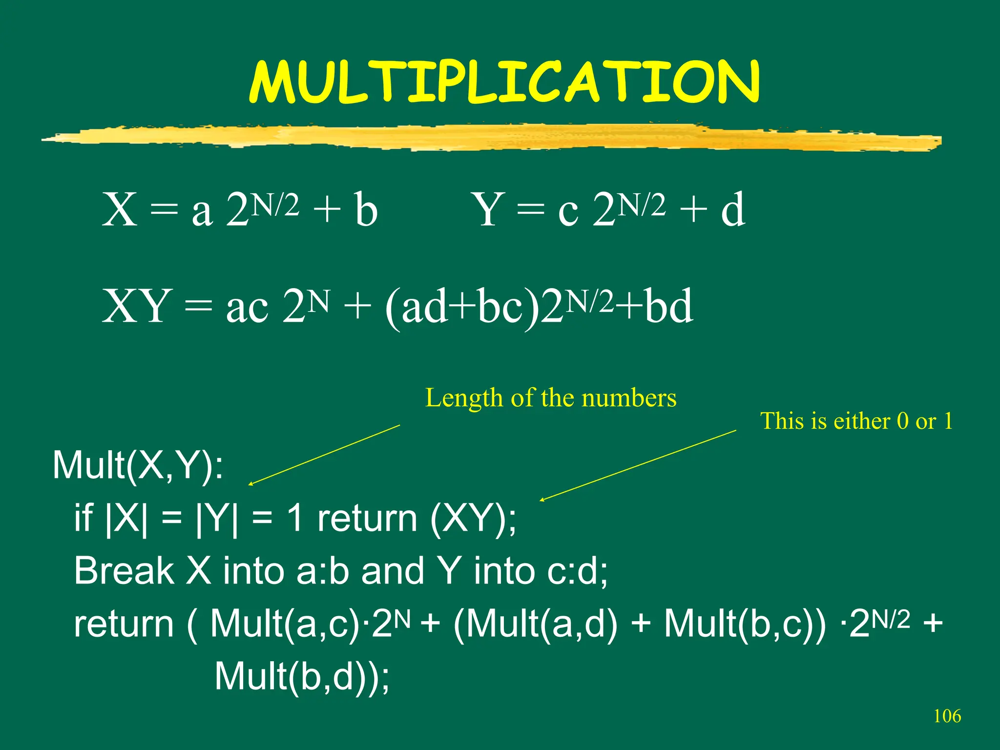
MULTIPLICATION
X = a2N/2 + b Y = c 2N/2 + d
XY = ac 2N + (ad+bc)2N/2+bd
Mult(X,Y):
if |X| = |Y| = 1 return (XY);
Break X into a:b and Y into c:d;
return ( Mult(a,c)·2N + (Mult(a,d) + Mult(b,c)) ·2N/2 +
Mult(b,d));
Length of the numbers
This is either 0 or 1
107.
107
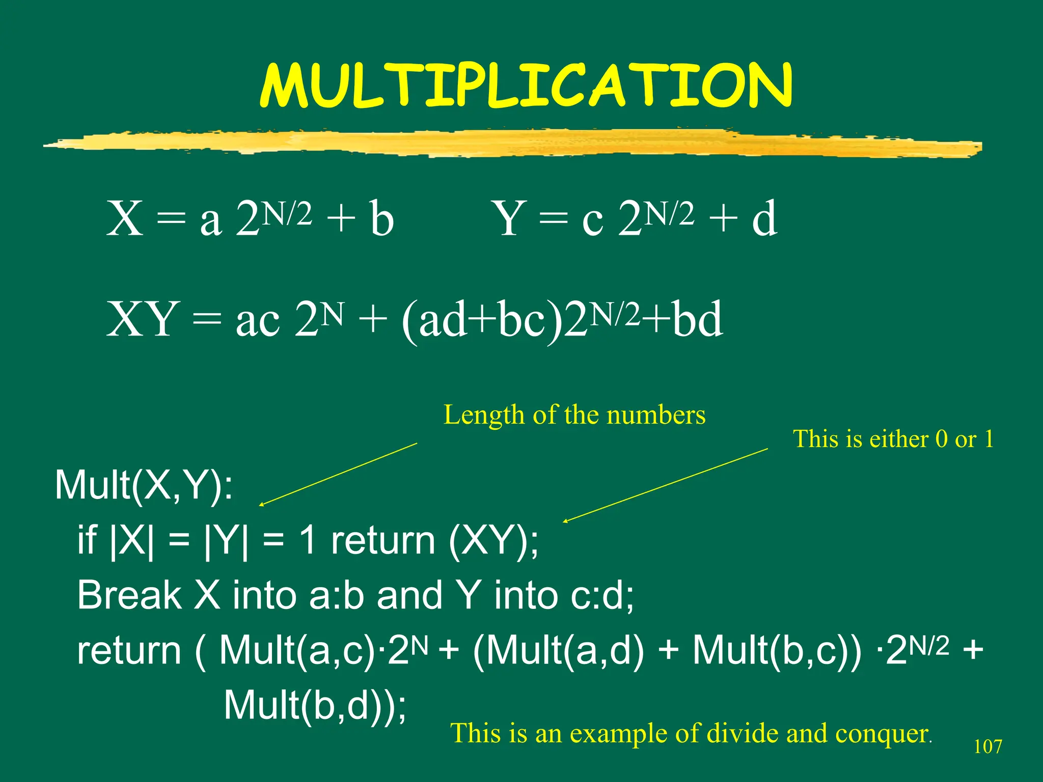
MULTIPLICATION
X = a2N/2 + b Y = c 2N/2 + d
XY = ac 2N + (ad+bc)2N/2+bd
Mult(X,Y):
if |X| = |Y| = 1 return (XY);
Break X into a:b and Y into c:d;
return ( Mult(a,c)·2N + (Mult(a,d) + Mult(b,c)) ·2N/2 +
Mult(b,d));
Length of the numbers
This is either 0 or 1
This is an example of divide and conquer.
108.
108
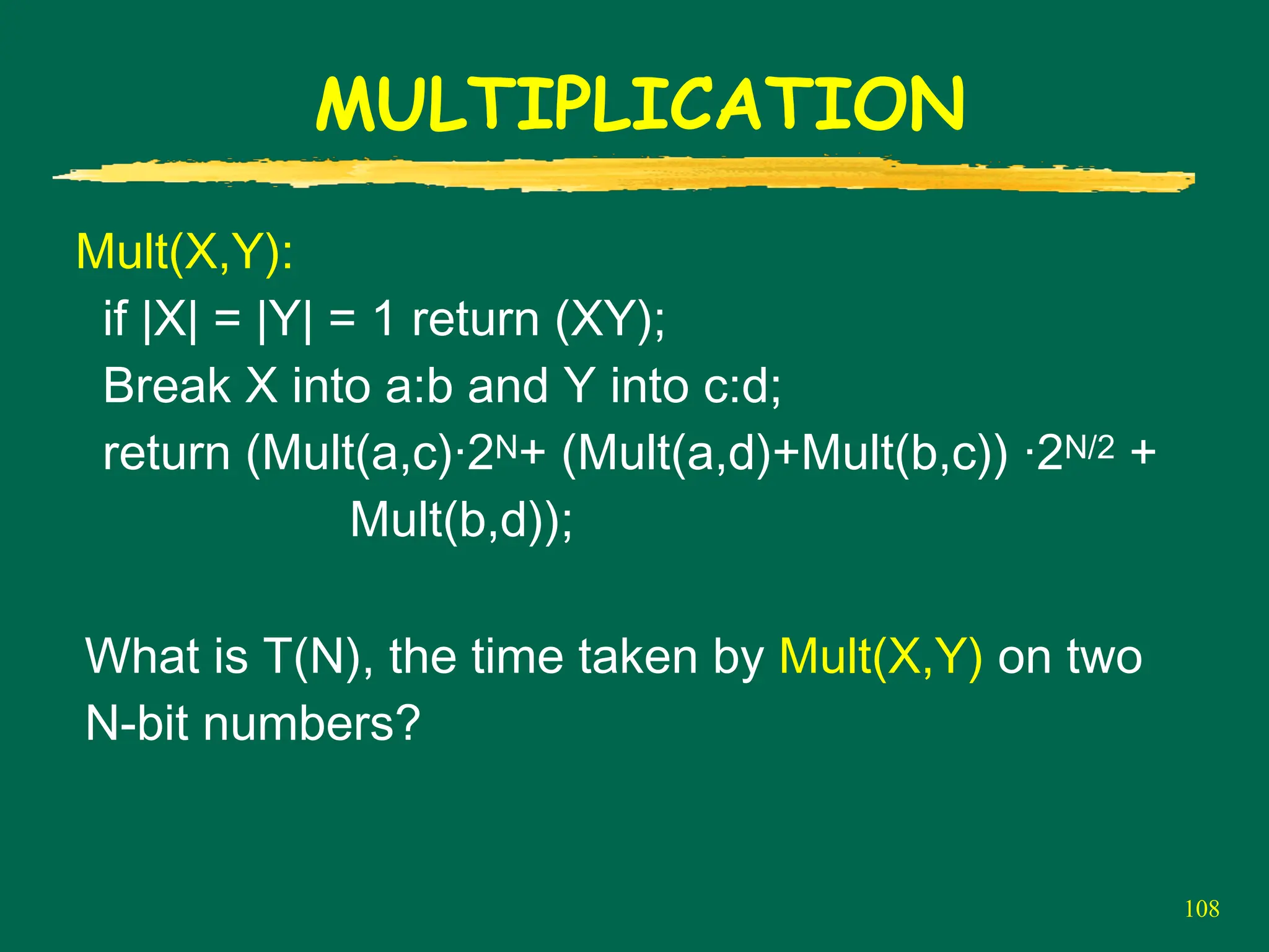
MULTIPLICATION
Mult(X,Y):
if |X| =|Y| = 1 return (XY);
Break X into a:b and Y into c:d;
return (Mult(a,c)·2N+ (Mult(a,d)+Mult(b,c)) ·2N/2 +
Mult(b,d));
What is T(N), the time taken by Mult(X,Y) on two
N-bit numbers?
109.
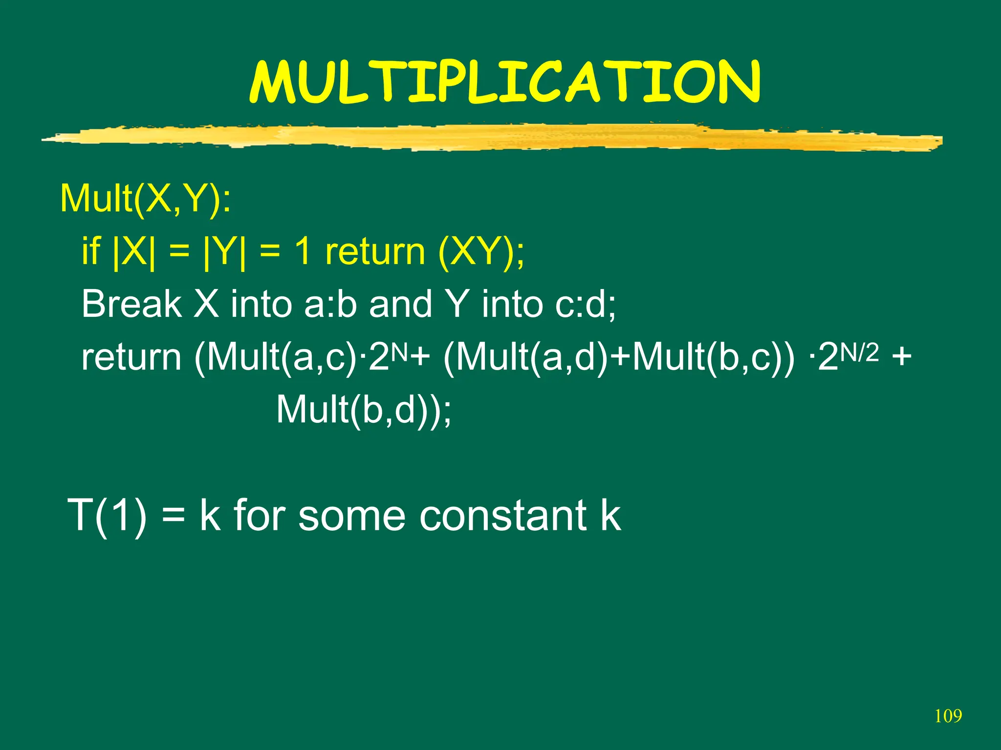
109
MULTIPLICATION
Mult(X,Y):
if |X| =|Y| = 1 return (XY);
Break X into a:b and Y into c:d;
return (Mult(a,c)·2N+ (Mult(a,d)+Mult(b,c)) ·2N/2 +
Mult(b,d));
T(1) = k for some constant k
110.
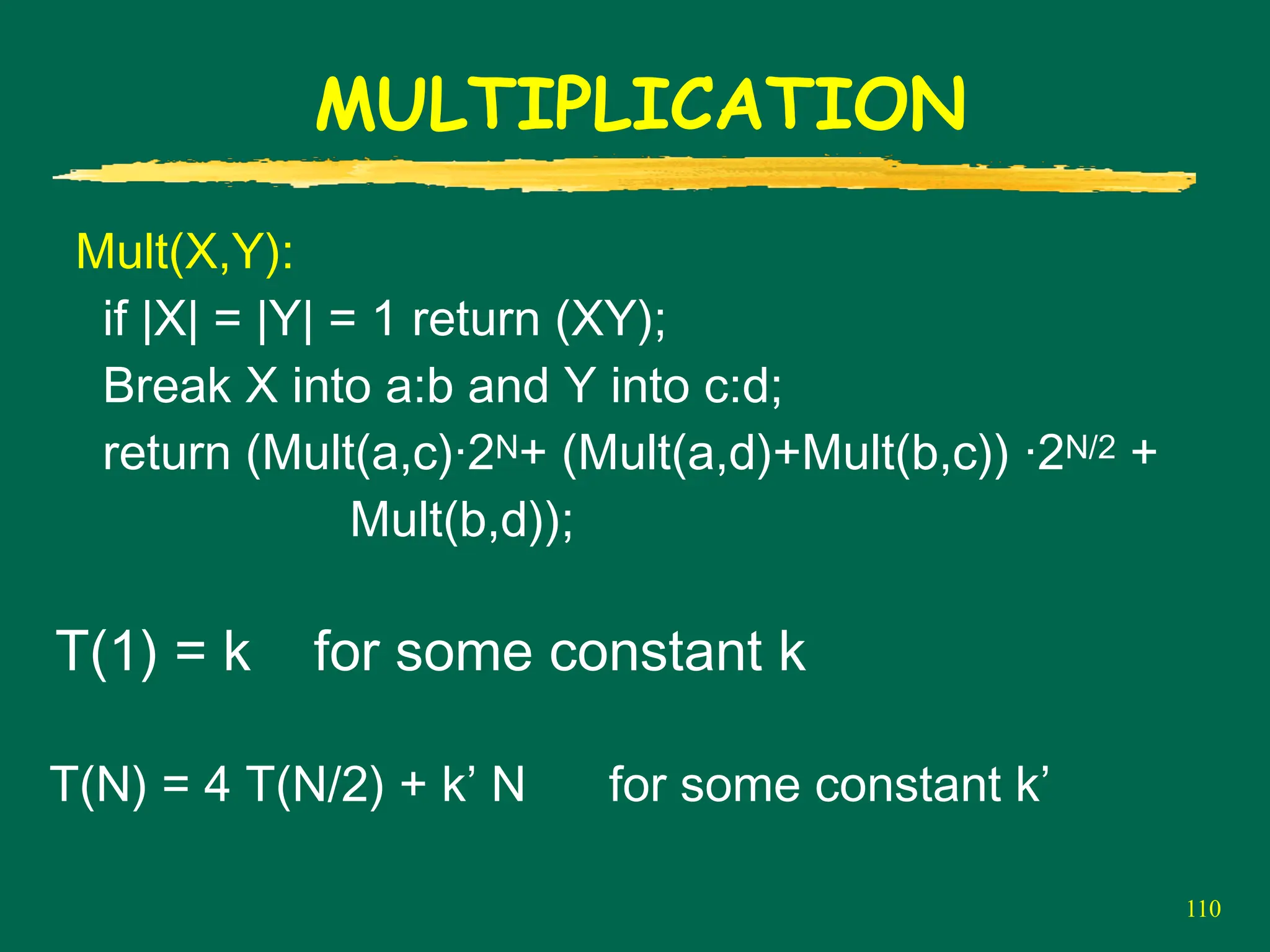
110
MULTIPLICATION
Mult(X,Y):
if |X| =|Y| = 1 return (XY);
Break X into a:b and Y into c:d;
return (Mult(a,c)·2N+ (Mult(a,d)+Mult(b,c)) ·2N/2 +
Mult(b,d));
T(1) = k for some constant k
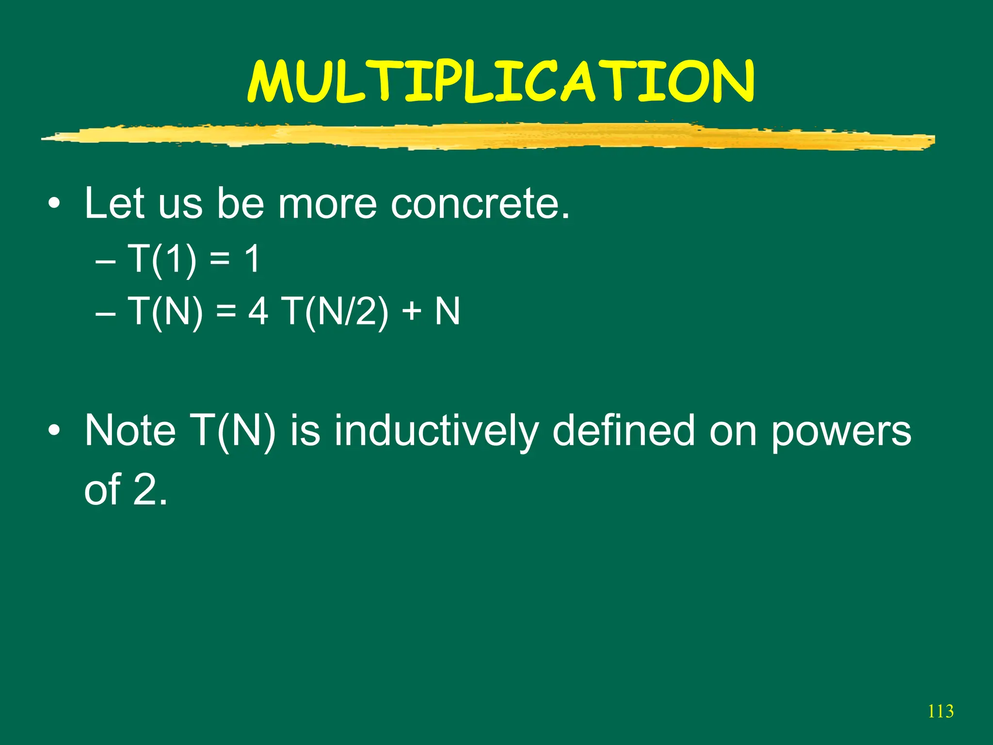
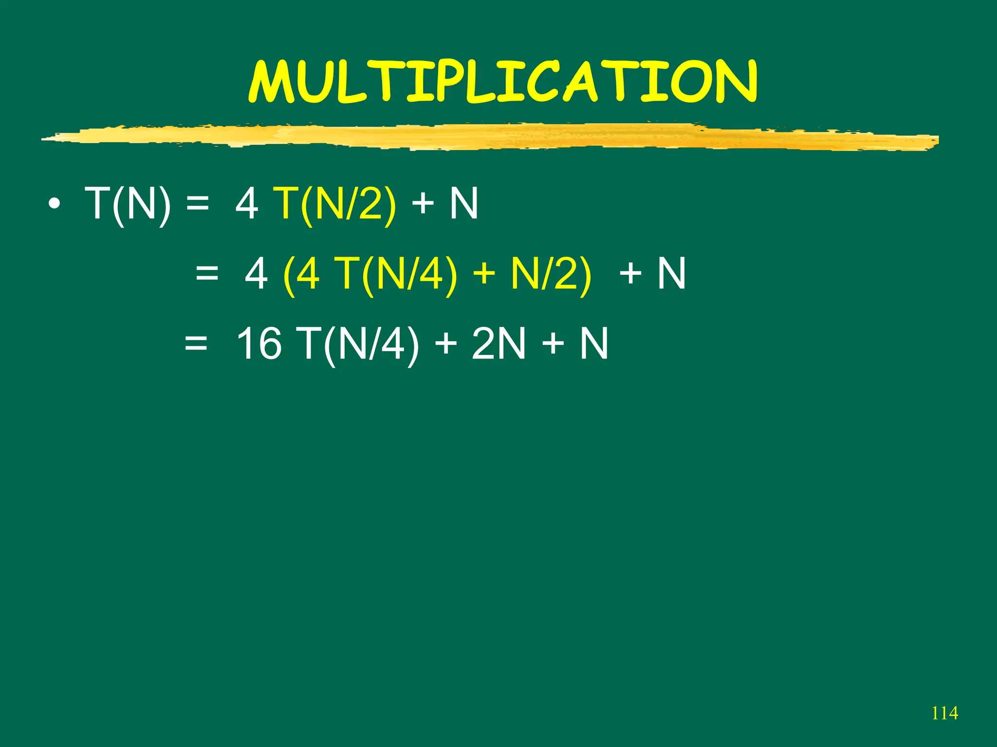
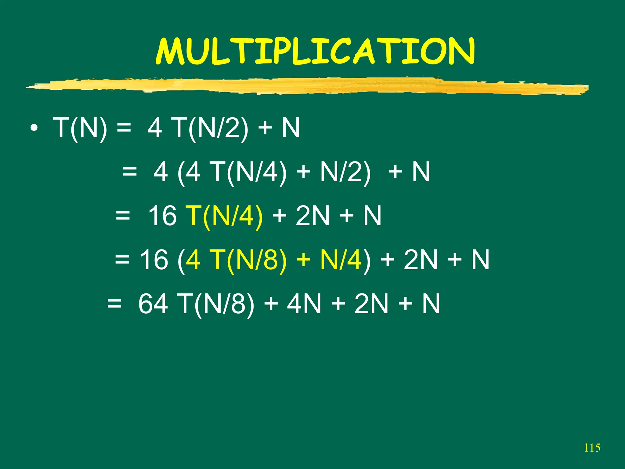
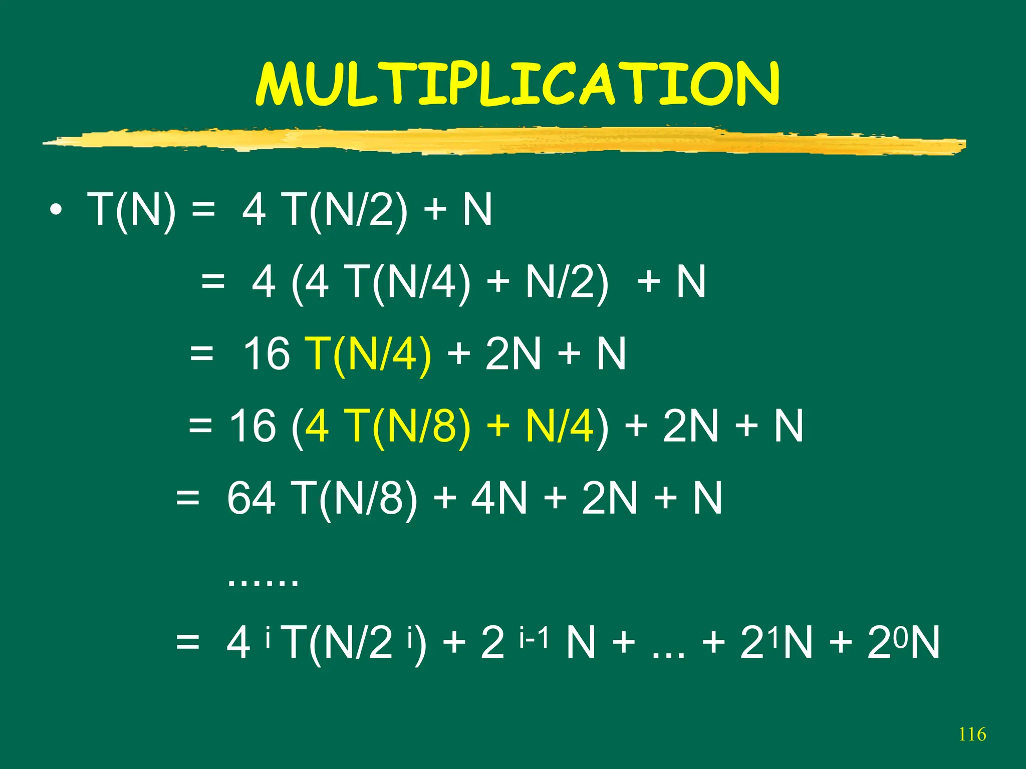
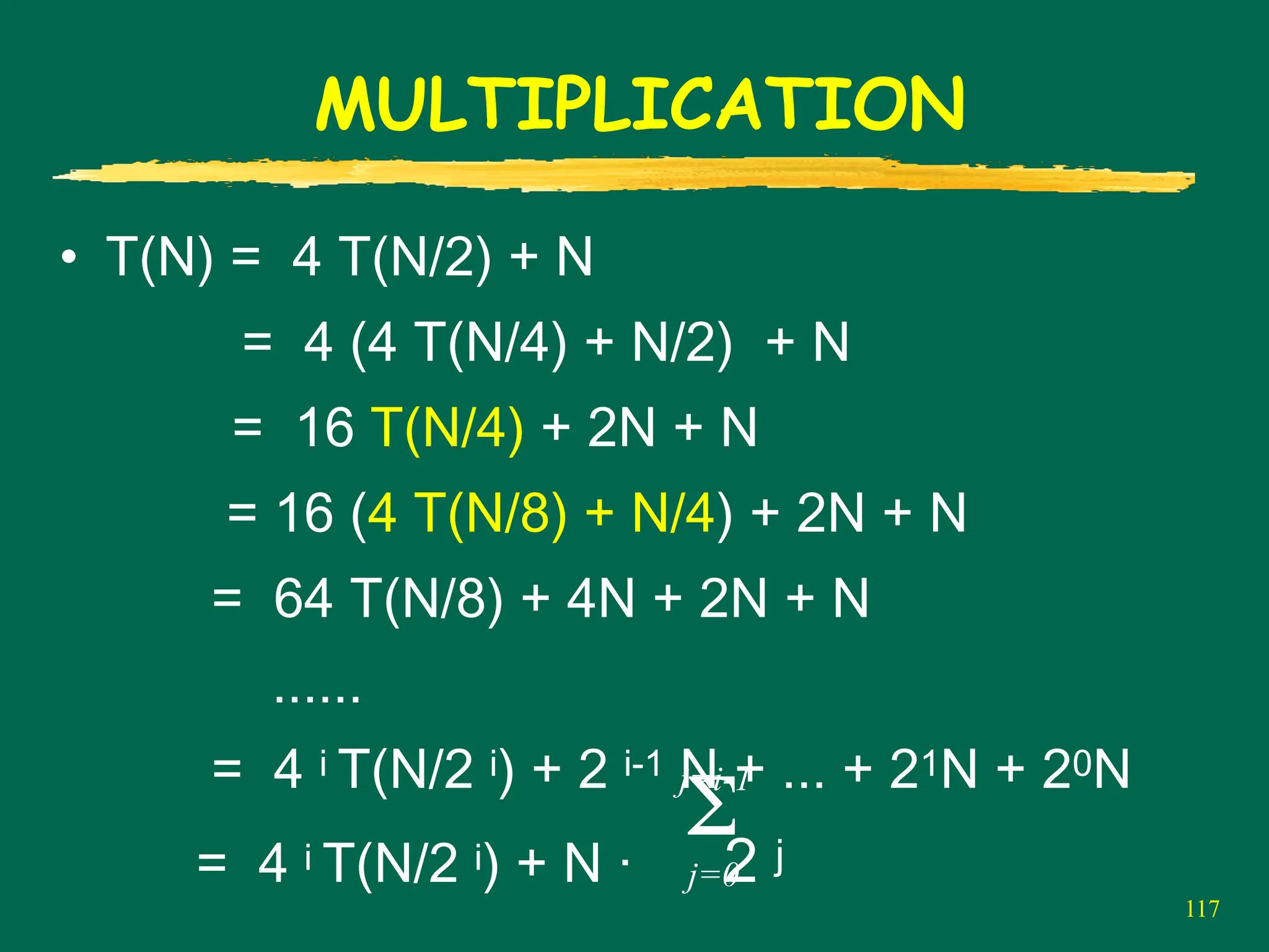
T(N) = 4 T(N/2) + k’ N for some constant k’
111.
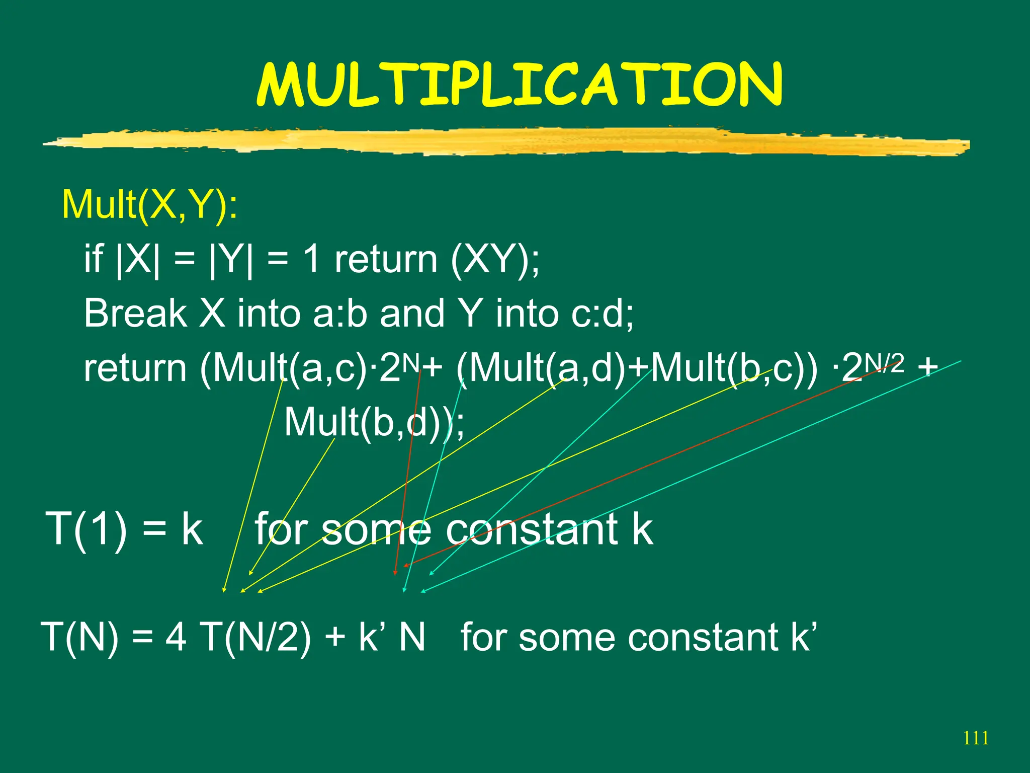
111
MULTIPLICATION
Mult(X,Y):
if |X| =|Y| = 1 return (XY);
Break X into a:b and Y into c:d;
return (Mult(a,c)·2N+ (Mult(a,d)+Mult(b,c)) ·2N/2 +
Mult(b,d));
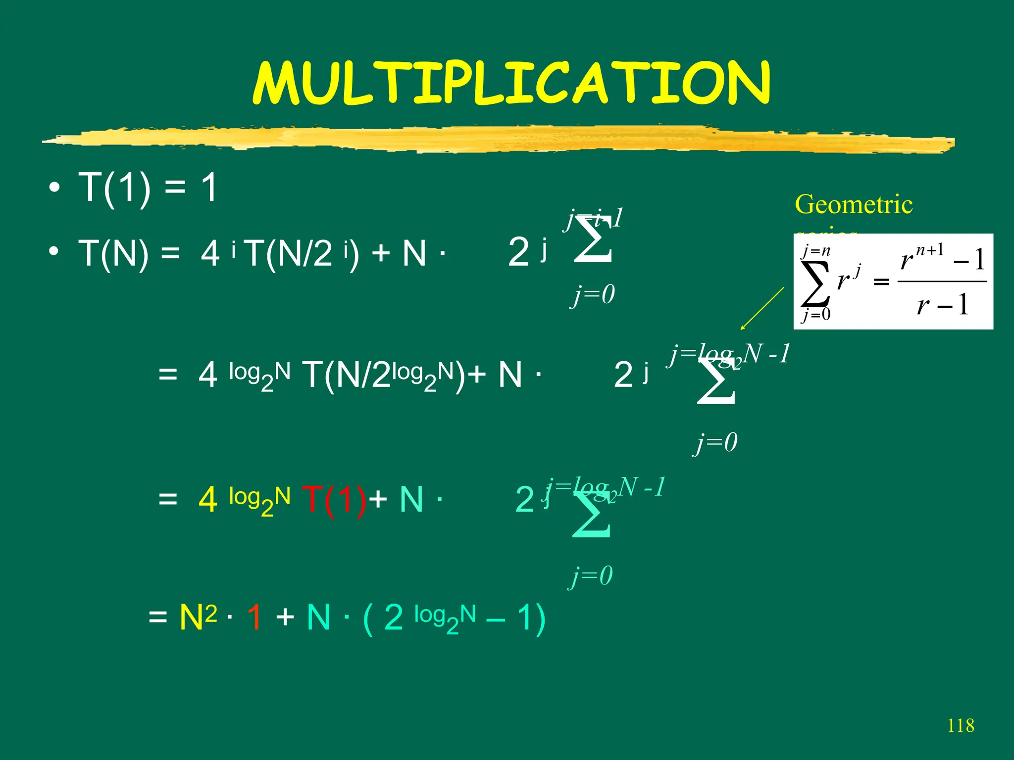
T(1) = k for some constant k
T(N) = 4 T(N/2) + k’ N for some constant k’
120
MULTIPLICATION
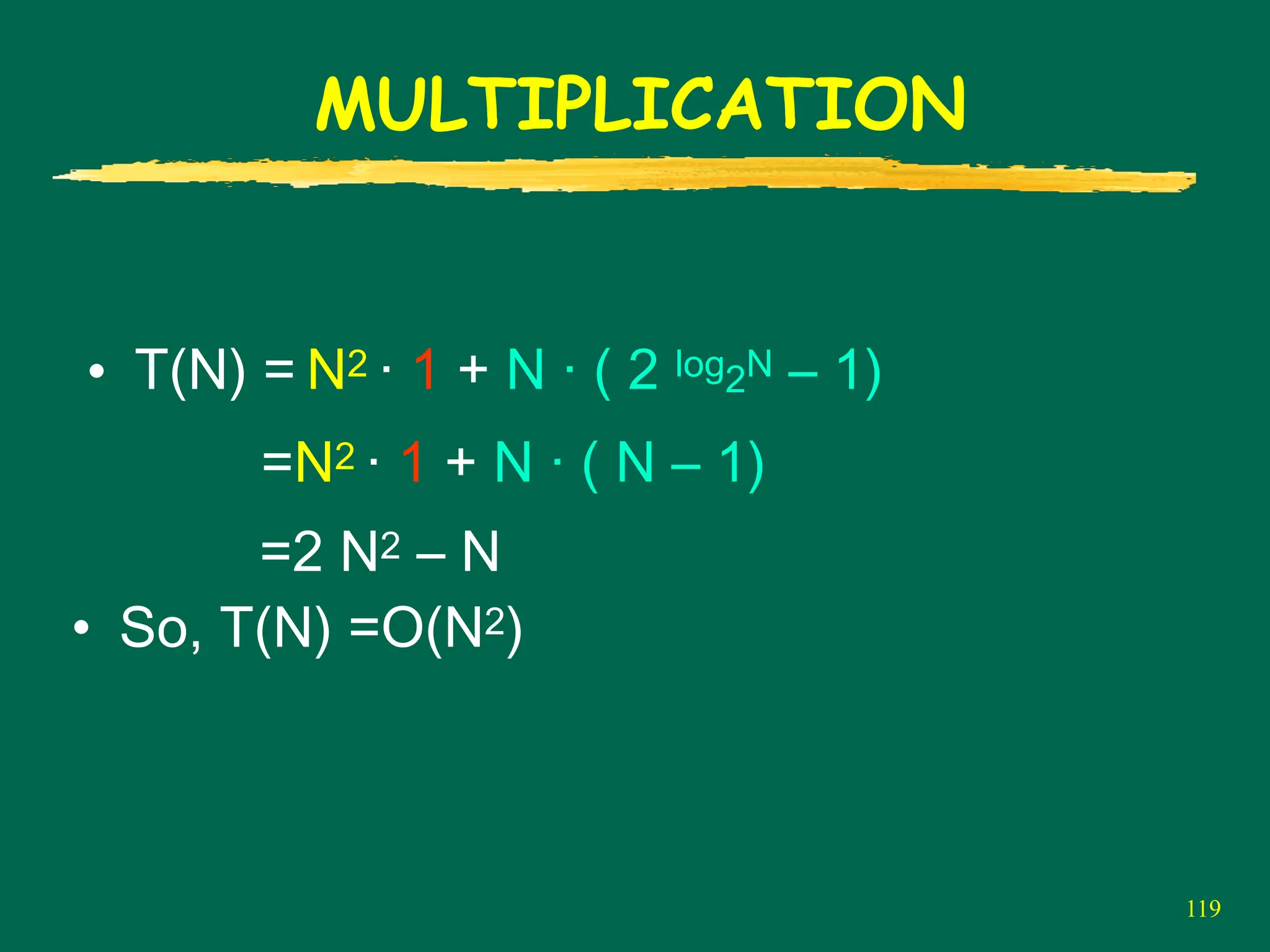
• T(N) =O(N2)
• Looks like divide and conquer did not buy us
anything.
• All that work for nothing!
121.
121
MULTIPLICATION
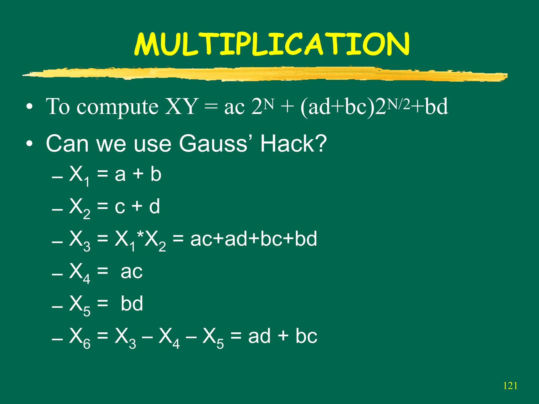
• To computeXY = ac 2N + (ad+bc)2N/2+bd
• Can we use Gauss’ Hack?
– X1 = a + b
– X2 = c + d
– X3 = X1*X2 = ac+ad+bc+bd
– X4 = ac
– X5 = bd
– X6 = X3 – X4 – X5 = ad + bc
122.
122
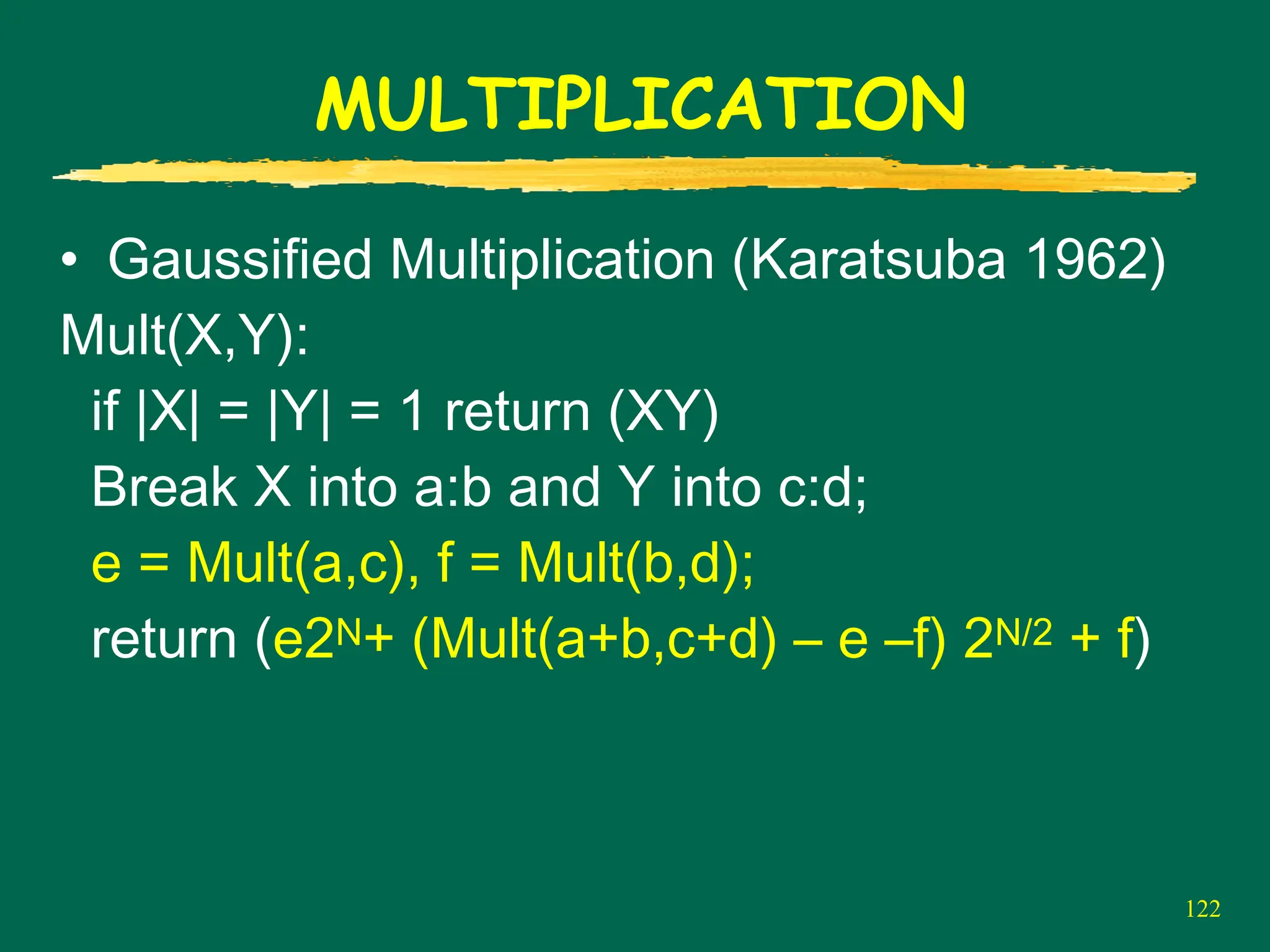
MULTIPLICATION
• Gaussified Multiplication(Karatsuba 1962)
Mult(X,Y):
if |X| = |Y| = 1 return (XY)
Break X into a:b and Y into c:d;
e = Mult(a,c), f = Mult(b,d);
return (e2N+ (Mult(a+b,c+d) – e –f) 2N/2 + f)
123.
123
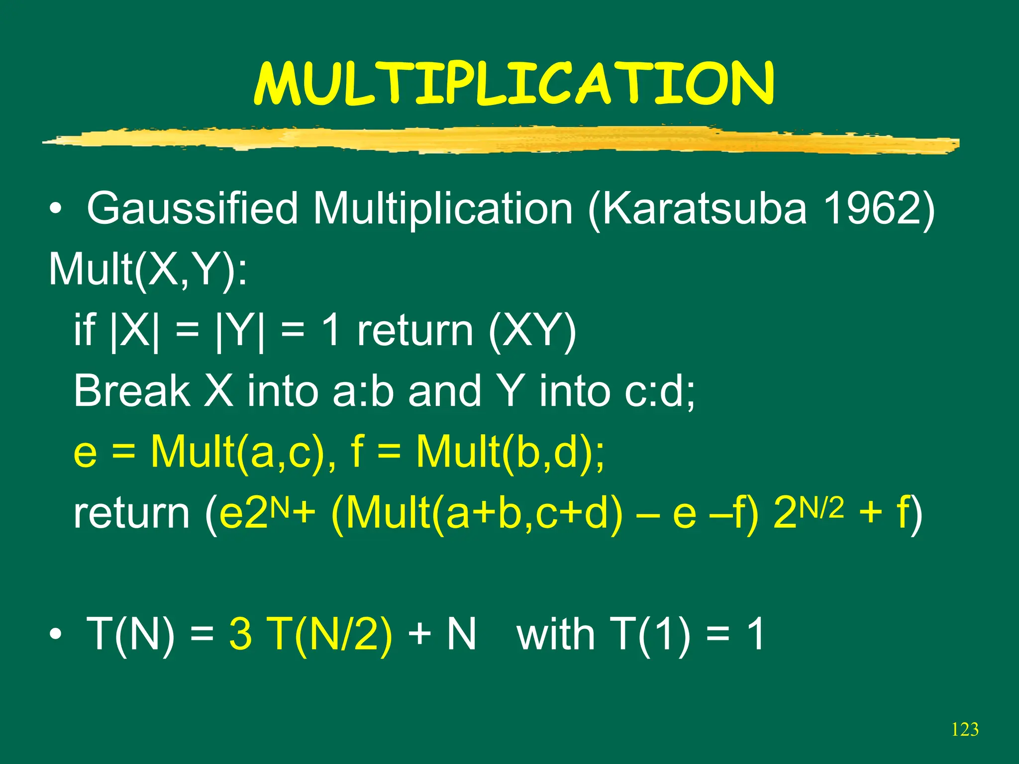
MULTIPLICATION
• Gaussified Multiplication(Karatsuba 1962)
Mult(X,Y):
if |X| = |Y| = 1 return (XY)
Break X into a:b and Y into c:d;
e = Mult(a,c), f = Mult(b,d);
return (e2N+ (Mult(a+b,c+d) – e –f) 2N/2 + f)
• T(N) = 3 T(N/2) + N with T(1) = 1
124.
124
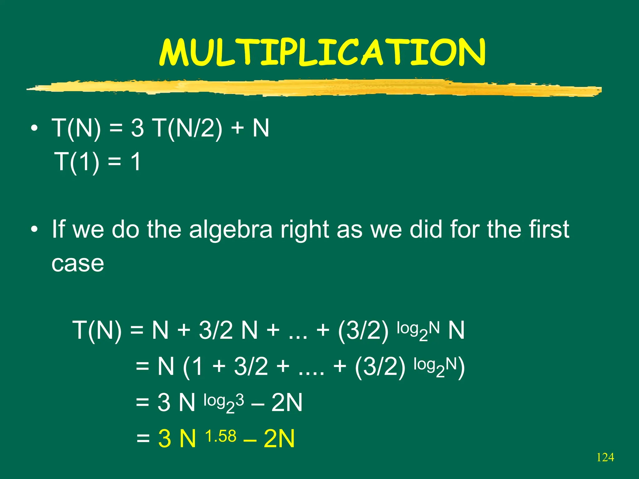
MULTIPLICATION
• T(N) =3 T(N/2) + N
T(1) = 1
• If we do the algebra right as we did for the first
case
T(N) = N + 3/2 N + ... + (3/2) log2N N
= N (1 + 3/2 + .... + (3/2) log2N)
= 3 N log23 – 2N
= 3 N 1.58 – 2N
125.
125
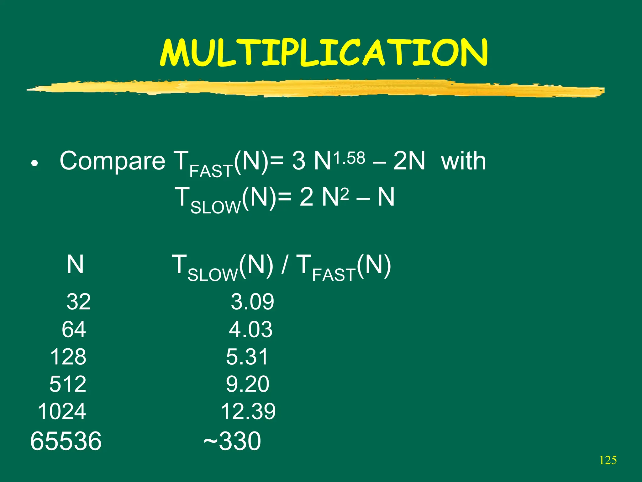
MULTIPLICATION
• Compare TFAST(N)=3 N1.58 – 2N with
TSLOW(N)= 2 N2 – N
N TSLOW(N) / TFAST(N)
32 3.09
64 4.03
128 5.31
512 9.20
1024 12.39
65536 ~330
127
FAST MULTIPLICATION
• Whyis this important?
• Modern cryptography systems (RSA,DES
etc) require multiplication of very large
numbers (1024 bit or 2048 bit).
• The fast multiplication algorithm improves
these systems substantially.
129
REVIEW and SOMECLOSING CONCEPTS
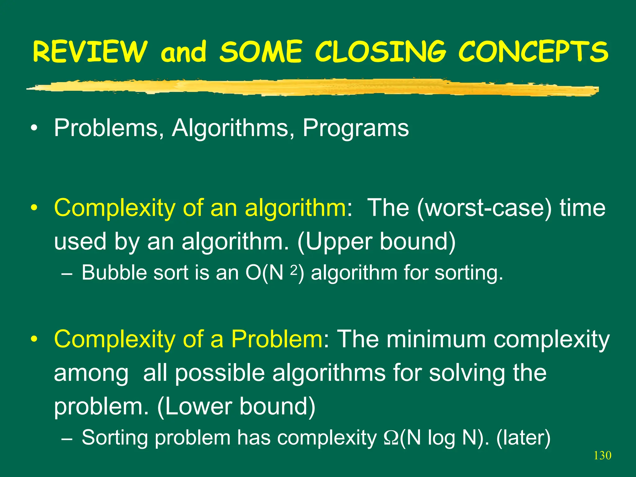
• Problems, Algorithms, Programs
• Complexity of an algorithm: The (worst-
case) time used by an algorithm.
– Bubble sort is an O(N 2) algorithm for sorting.
130.
130
REVIEW and SOMECLOSING CONCEPTS
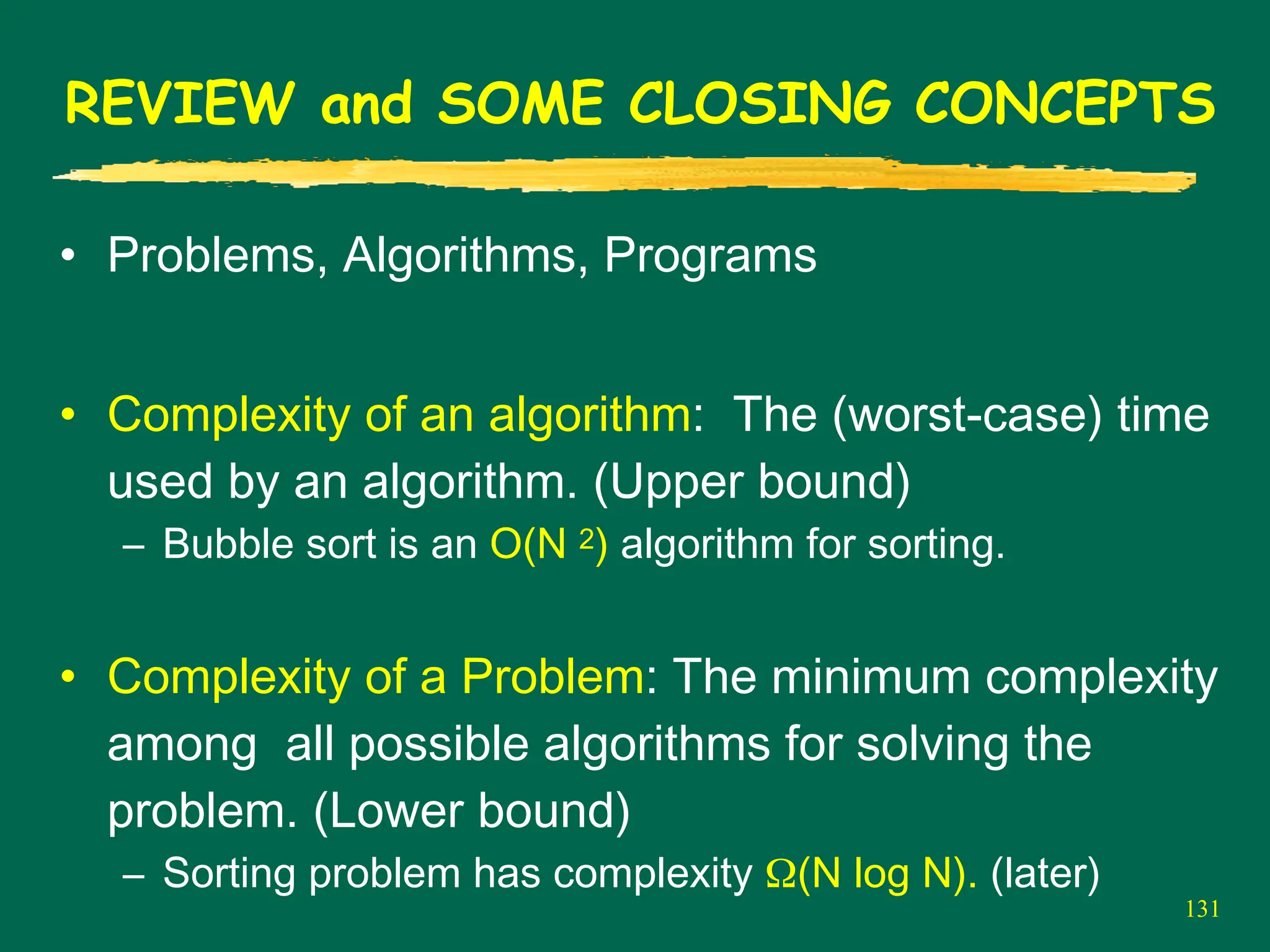
• Problems, Algorithms, Programs
• Complexity of an algorithm: The (worst-case) time
used by an algorithm. (Upper bound)
– Bubble sort is an O(N 2) algorithm for sorting.
• Complexity of a Problem: The minimum complexity
among all possible algorithms for solving the
problem. (Lower bound)
– Sorting problem has complexity Ω(N log N). (later)
131.
131
REVIEW and SOMECLOSING CONCEPTS
• Problems, Algorithms, Programs
• Complexity of an algorithm: The (worst-case) time
used by an algorithm. (Upper bound)
– Bubble sort is an O(N 2) algorithm for sorting.
• Complexity of a Problem: The minimum complexity
among all possible algorithms for solving the
problem. (Lower bound)
– Sorting problem has complexity Ω(N log N). (later)
132.
132
REVIEW and SOMECLOSING CONCEPTS
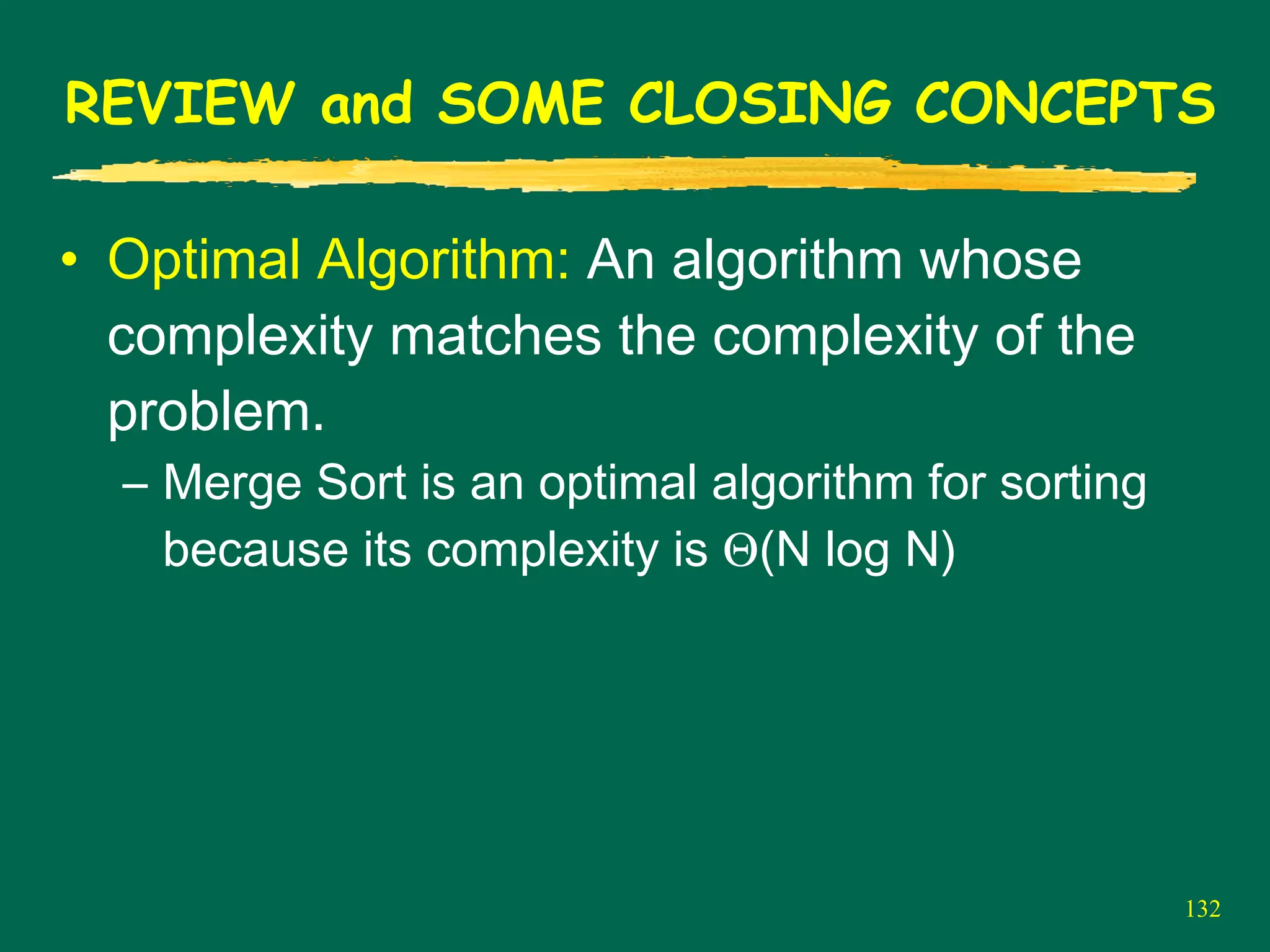
• Optimal Algorithm: An algorithm whose
complexity matches the complexity of the
problem.
– Merge Sort is an optimal algorithm for sorting
because its complexity is Θ(N log N)


![39
AN EXAMPLE
{
1 int i,j;
2 for(i=1; i <= n ; i=i*2) {
3 for(j = 0; j < i; j++) {
4 foo[i][j] = 0;
5 for (k = 0; k < n; k++) {
6 foo[i][j] = bar[k][i+j] + foo[i][j];
7 }
8 }
9 }
}
O(1) O(n)
O(1)
O(n)](https://image.slidesharecdn.com/2-algorithmsanalysis-251210134652-369fc7d7/75/uploaed-noducment-file-docudnet-bgood-notes-39-2048.jpg)
![40
AN EXAMPLE
{
1 int i,j;
2 for(i=1; i <= n ; i=i*2) {
3 for(j = 0; j < i; j++) {
4 foo[i][j] = 0;
5 for (k = 0; k < n; k++) {
6 foo[i][j] = bar[k][i+j] + foo[i][j];
7 }
8 }
9 }
}
O(n)
O(i•n)](https://image.slidesharecdn.com/2-algorithmsanalysis-251210134652-369fc7d7/75/uploaed-noducment-file-docudnet-bgood-notes-40-2048.jpg)
![41
AN EXAMPLE
{
1 int i,j;
2 for(i=1; i <= n ; i=i*2) {
3 for(j = 0; j < i; j++) {
4 foo[i][j] = 0;
5 for (k = 0; k < n; k++) {
6 foo[i][j] = bar[k][i+j] + foo[i][j];
7 }
8 }
9 }
}
O(n)
O(i•n)
Although this loop is executed about log n times,
at each iteration the time of the inner loop
changes!](https://image.slidesharecdn.com/2-algorithmsanalysis-251210134652-369fc7d7/75/uploaed-noducment-file-docudnet-bgood-notes-41-2048.jpg)
![42
AN EXAMPLE
{
1 int i,j;
2 for(i=1; i <= n ; i=i*2) {
3 for(j = 0; j < i; j++) {
4 foo[i][j] = 0;
5 for (k = 0; k < n; k++) {
6 foo[i][j] = bar[k][i+j] + foo[i][j];
7 }
8 }
9 }
}
O(n)
O(i•n)
Although this loop is executed about log n times,
at each iteration the time of the inner loop
changes!](https://image.slidesharecdn.com/2-algorithmsanalysis-251210134652-369fc7d7/75/uploaed-noducment-file-docudnet-bgood-notes-42-2048.jpg)
![57
COMPUTING FIBONACCI NUMBERS
• The next obvious algorithm (assume n ≥ 0)
int fib( int n)
{int X[3];
if (n <= 1) return(n);
X[0]=0; X[1]=1;
for (i = 2; i <= n; i++)
X[i % 3] = X[(i-1) % 3] + X[(i-2) % 3];
return X[(i-1)%3] ;
}](https://image.slidesharecdn.com/2-algorithmsanalysis-251210134652-369fc7d7/75/uploaed-noducment-file-docudnet-bgood-notes-57-2048.jpg)
![58
COMPUTING FIBONACCI NUMBERS
• The next obvious algorithm (assume n ≥ 0)
int fib( int n)
{int X[3];
if (n <= 1) return(n);
X[0]=0; X[1]=1;
for (i = 2; i <= n; i++)
X[i % 3] = X[(i-1) % 3] + X[(i-2) % 3];
return X[(i-1)%3] ;
}
• % is the mod operator i%3 ≡ i mod 3](https://image.slidesharecdn.com/2-algorithmsanalysis-251210134652-369fc7d7/75/uploaed-noducment-file-docudnet-bgood-notes-58-2048.jpg)
![59
COMPUTING FIBONACCI NUMBERS
• The next obvious algorithm (assume n ≥ 0)
int fib( int n)
{int X[3];
if (n <= 1) return(n);
X[0]=0; X[1]=1;
for (i = 2; i <= n; i++)
X[i % 3] = X[(i-1) % 3] + X[(i-2) % 3];
return X[(i-1)%3] ;
}
0
1
X[0]
X[1]
X[2]
when i=2
fib(0)
fib(1)](https://image.slidesharecdn.com/2-algorithmsanalysis-251210134652-369fc7d7/75/uploaed-noducment-file-docudnet-bgood-notes-59-2048.jpg)
![60
COMPUTING FIBONACCI NUMBERS
• The next obvious algorithm (assume n ≥ 0)
int fib( int n)
{int X[3];
if (n <= 1) return(n);
X[0]=0; X[1]=1;
for (i = 2; i <= n; i++)
X[i % 3] = X[(i-1) % 3] + X[(i-2) % 3];
return X[(i-1)%3] ;
}
0
1
1
X[0]
X[1]
X[2]
fib(2) fib(1)
fib(0)](https://image.slidesharecdn.com/2-algorithmsanalysis-251210134652-369fc7d7/75/uploaed-noducment-file-docudnet-bgood-notes-60-2048.jpg)
![61
COMPUTING FIBONACCI NUMBERS
• The next obvious algorithm (assume n ≥ 0)
int fib( int n)
{int X[3];
if (n <= 1) return(n);
X[0]=0; X[1]=1;
for (i = 2; i <= n; i++)
X[i % 3] = X[(i-1) % 3] + X[(i-2) % 3];
return X[(i-1)%3] ;
}
2
1
1
X[0]
X[1]
X[2]
fib(3)
fib(2) fib(1)](https://image.slidesharecdn.com/2-algorithmsanalysis-251210134652-369fc7d7/75/uploaed-noducment-file-docudnet-bgood-notes-61-2048.jpg)
![62
COMPUTING FIBONACCI NUMBERS
• The next obvious algorithm (assume n ≥ 0)
int fib( int n)
{int X[3];
if (n <= 1) return(n);
X[0]=0; X[1]=1;
for (i = 2; i <= n; i++)
X[i % 3] = X[(i-1) % 3] + X[(i-2) % 3];
return X[(i-1)%3] ;
}
2
3
1
X[0]
X[1]
X[2]
fib(4)
fib(3)
fib(2)](https://image.slidesharecdn.com/2-algorithmsanalysis-251210134652-369fc7d7/75/uploaed-noducment-file-docudnet-bgood-notes-62-2048.jpg)
![63
COMPUTING FIBONACCI NUMBERS
• The next obvious algorithm (assume n ≥ 0)
int fib( int n)
{int X[3];
if (n <= 1) return(n);
X[0]=0; X[1]=1;
for (i = 2; i <= n; i++)
X[i % 3] = X[(i-1) % 3] + X[(i-2) % 3];
return X[(i-1)%3] ;
}
2
3
5
X[0]
X[1]
X[2]
fib(5)](https://image.slidesharecdn.com/2-algorithmsanalysis-251210134652-369fc7d7/75/uploaed-noducment-file-docudnet-bgood-notes-63-2048.jpg)
![64
COMPUTING FIBONACCI NUMBERS
• The next obvious algorithm (assume n ≥ 0)
int fib( int n)
{int X[3];
if (n <= 1) return(n);
X[0]=0; X[1]=1;
for (i = 2; i <= n; i++)
X[i % 3] = X[(i-1) % 3] + X[(i-2) % 3];
return X[(i-1)%3] ; (Why?)
}
• Because i is incremented at the end of the loop
before exit.](https://image.slidesharecdn.com/2-algorithmsanalysis-251210134652-369fc7d7/75/uploaed-noducment-file-docudnet-bgood-notes-64-2048.jpg)
![65
COMPUTING FIBONACCI NUMBERS
• The next obvious algorithm (assume n ≥ 0)
int fib( int n)
{int X[3];
if (n <= 1) return(n);
X[0]=0; X[1]=1;
for (i = 2; i <= n; i++)
X[i % 3] = X[(i-1) % 3] + X[(i-2) % 3];
return X[(i-1)%3] ;
}
• ~N iterations each taking constant time → O(N)](https://image.slidesharecdn.com/2-algorithmsanalysis-251210134652-369fc7d7/75/uploaed-noducment-file-docudnet-bgood-notes-65-2048.jpg)
![66
COMPUTING FIBONACCI NUMBERS
• The next obvious algorithm (assume n ≥ 0)
int fib( int n)
{int X[3];
if (n <= 1) return(n);
X[0]=0; X[1]=1;
for (i = 2; i <= n; i++)
X[i % 3] = X[(i-1) % 3] + X[(i-2) % 3];
return X[(i-1)%3] ;
}
• ~N iterations each taking constant time → O(N)
• Much better than the O(cN) algorithm, but ....](https://image.slidesharecdn.com/2-algorithmsanalysis-251210134652-369fc7d7/75/uploaed-noducment-file-docudnet-bgood-notes-66-2048.jpg)