FUNDAMENTALS

1. .
“Introduction to Algorithm &
Data Structure”
.

2. Syllabus:
• Introduction: From Problem to Program (Problem, Solution, Algorithm,
Data Structure and Program). Data Structures: Data, Information,
Knowledge, and Data structure, Abstract Data Types (ADT), Data
• Structure Classification (Linear and Non-linear, Static and Dynamic,
Persistent and Ephemeral data
• structures).
• Algorithms: Problem Solving, Introduction to algorithm, Characteristics
of algorithm, Algorithm design tools: Pseudo-code and flowchart.
Complexity of algorithm: Space complexity, Time complexity,
Asymptotic notation- Big-O, Theta and Omega, finding complexity
using step count method, Analysis of programming constructs-Linear,
Quadratic, Cubic, Logarithmic. Algorithmic Strategies: Introduction to
algorithm design strategies- Divide and Conquer, and Greedy strategy.

3. WHY?
• They enable efficient data manipulation,
making it easier to preprocess and prepare
data for modeling.
• The choice of data structure often depends on
the nature of the data and the ML model
used.
• Understanding data dimensions helps you
grasp how your data evolves, improving
feature engineering and model design.

4. ALGORITHMS

5. ALGORITHM – PROBLEM SOLVING
COMPUTER :
“Computer is multi purpose Electronic Machine which is
used for storing , organizing and processing data by set of
program
Problem :
“Problem is defined as situation or condition which needs
to solve to achive goal”
Steps in Problem Solving :
1. Define the problem
2. Data gathering
3. Decide effective solution
4. Implement and evaluate the solution
5. Review the result.

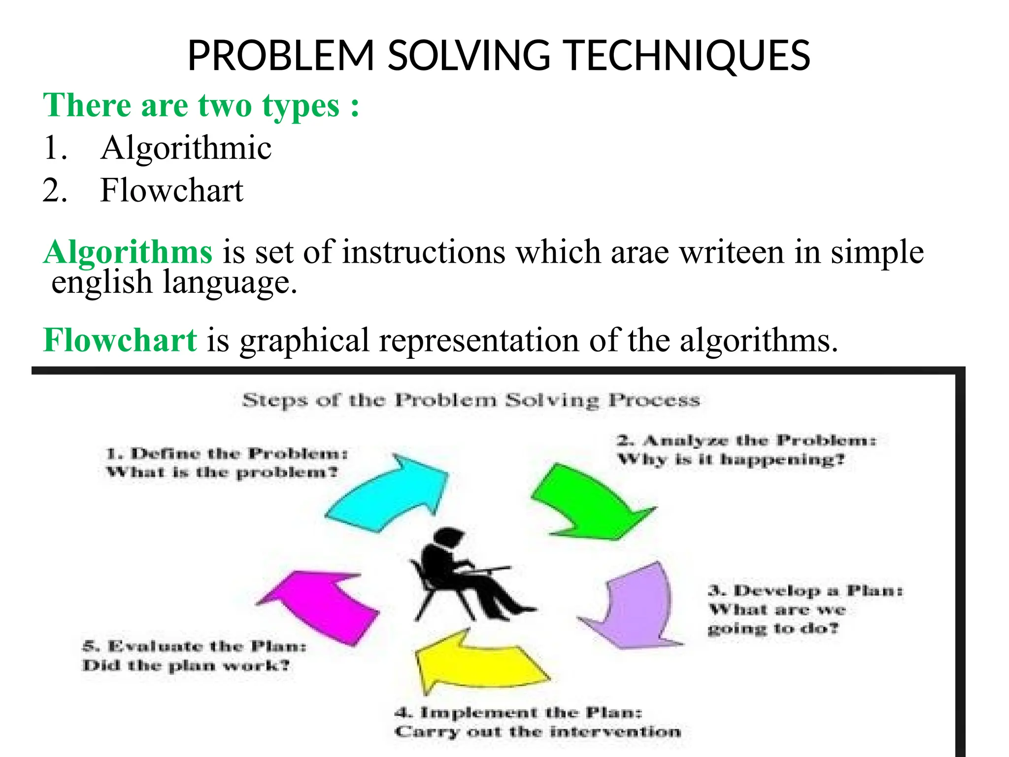
6. PROBLEM SOLVING TECHNIQUES
There are two types :
1. Algorithmic
2. Flowchart
Algorithms is set of instructions which arae writeen in simple
english language.
Flowchart is graphical representation of the algorithms.

7. Some other Problem Solving
Techniques
1. Trial and error techniques
2. Divide and conquer techniques
3. Merging solution
4. The building block approach
The building-block approach is a method for building confidence in
designs by working to develop understanding of behavior of lower-
level components, then using the knowledge gained to inform
representations of more complex assemblies.
5. Brain storming techniques
6. Solve by analogy.

8. Solve by analogy.
• Understand the relationship between the given pair of
words, phrases, or objects.
• Look for patterns in the given pair that can be applied to
the other pair.
• Analyze each answer choice and try to determine if it
follows the same relationship as the given pair.
• Formulate the relationship between the words in the given
word pair and then select the answer containing words
related to one another in most nearly the same way.

9. INTRODUCTION OF ALGORITHMS
DEFINITION :
“An algorithm is defined as a step-by-step procedure or method for
solving a problem by a computer in a finite number of steps.”
From the data structure point of view, following are some
important categories of algorithms −
Search − Algorithm to search an item in a data structure.
Sort − Algorithm to sort items in a certain order.
Insert − Algorithm to insert item in a data structure.
Update − Algorithm to update an existing item in a data
structure.
Delete − Algorithm to delete an existing item from a data

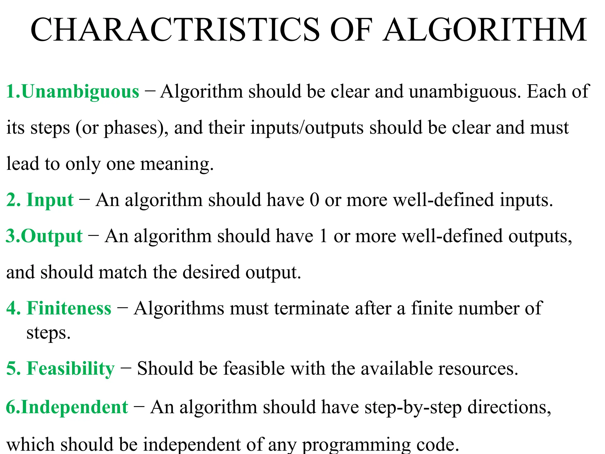
10. CHARACTRISTICS OF ALGORITHM
1.Unambiguous − Algorithm should be clear and unambiguous. Each of
its steps (or phases), and their inputs/outputs should be clear and must
lead to only one meaning.
2. Input − An algorithm should have 0 or more well-defined inputs.
3.Output − An algorithm should have 1 or more well-defined outputs,
and should match the desired output.
4. Finiteness − Algorithms must terminate after a finite number of
steps.
5. Feasibility − Should be feasible with the available resources.
6.Independent − An algorithm should have step-by-step directions,
which should be independent of any programming code.

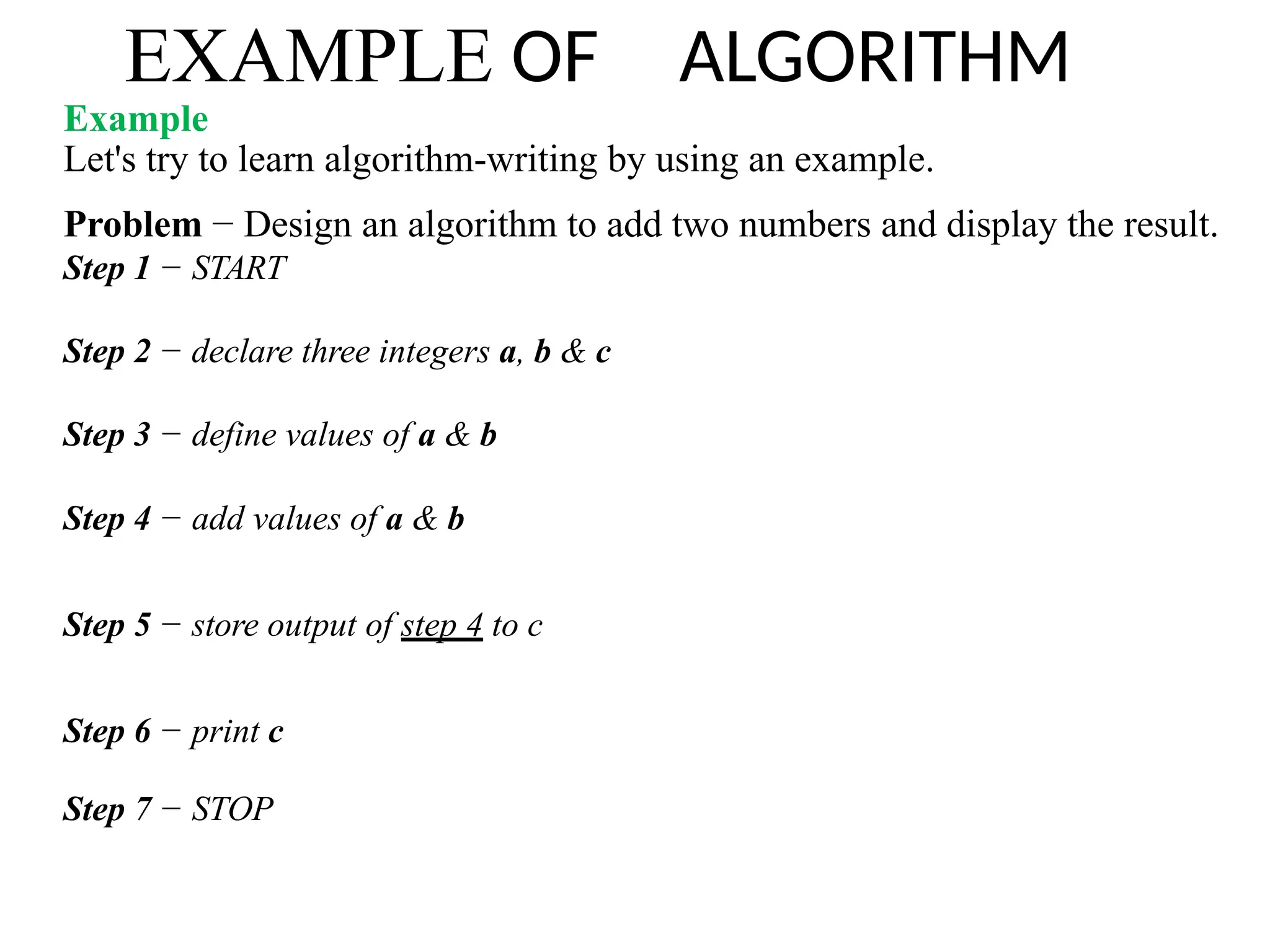
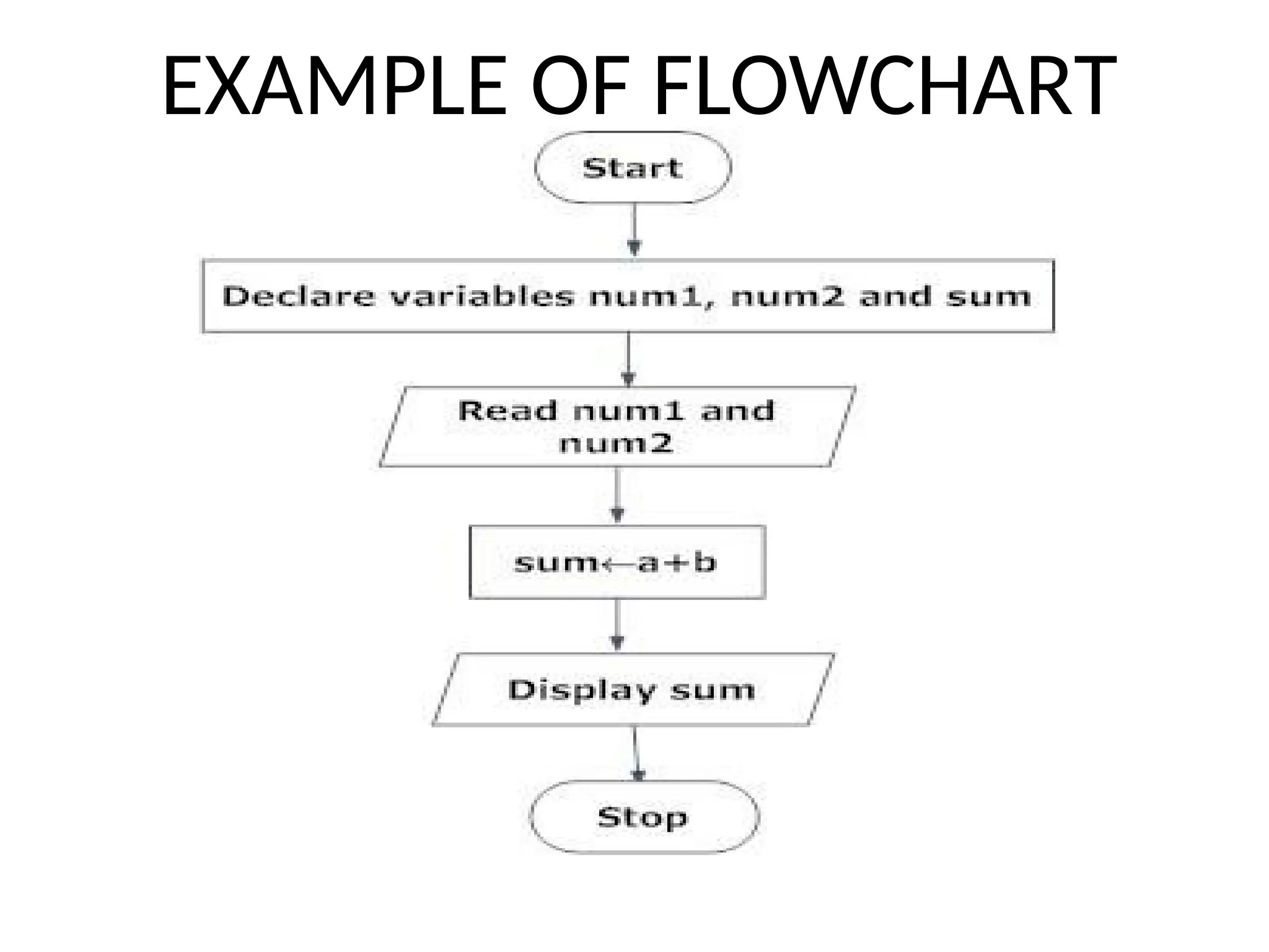
11. EXAMPLE OF ALGORITHM
Example
Let's try to learn algorithm-writing by using an example.
Problem − Design an algorithm to add two numbers and display the result.
Step 1 − START
Step 2 − declare three integers a, b & c
Step 3 − define values of a & b
Step 4 − add values of a & b
Step 5 − store output of step 4 to c
Step 6 − print c
Step 7 − STOP

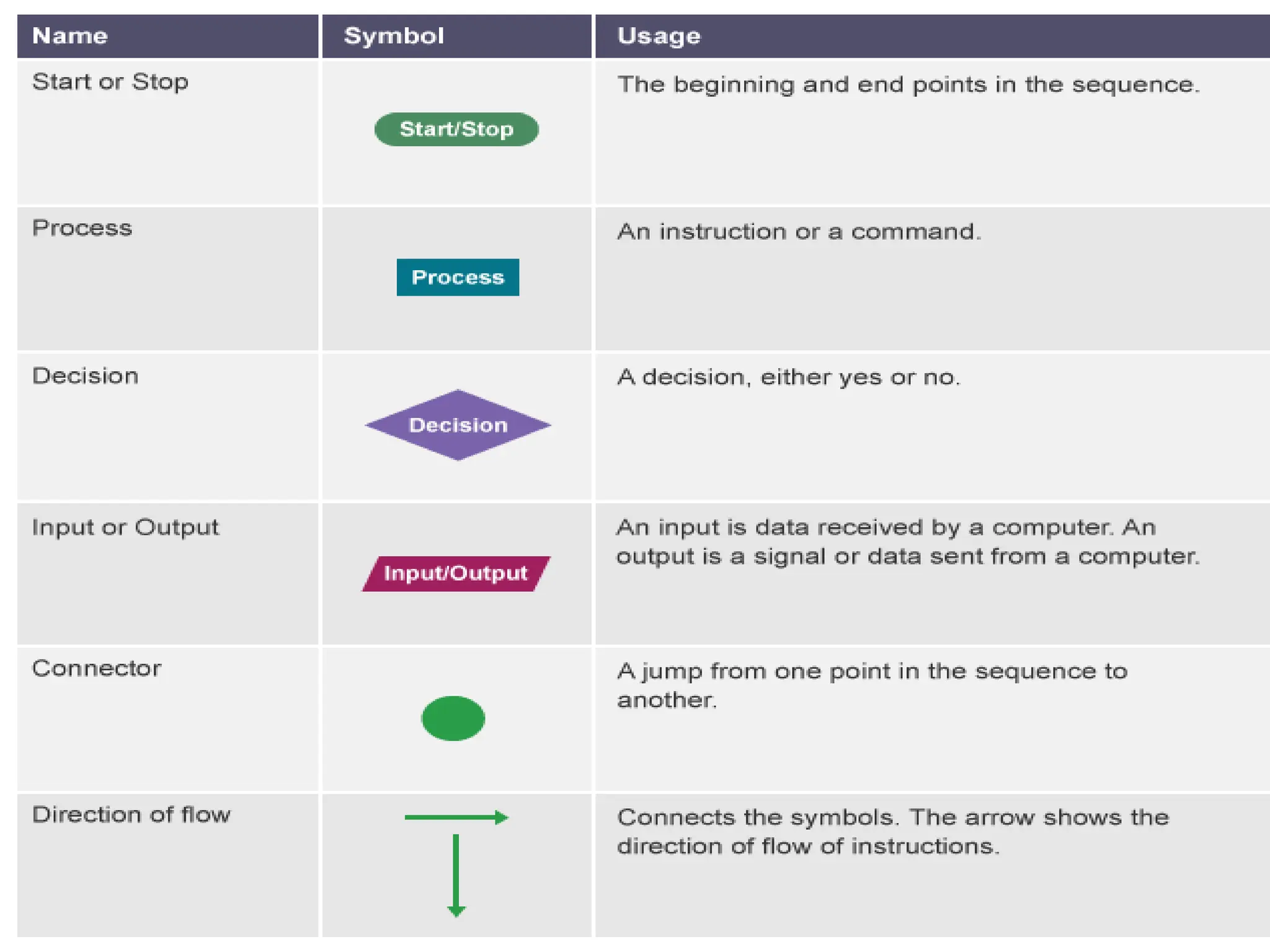
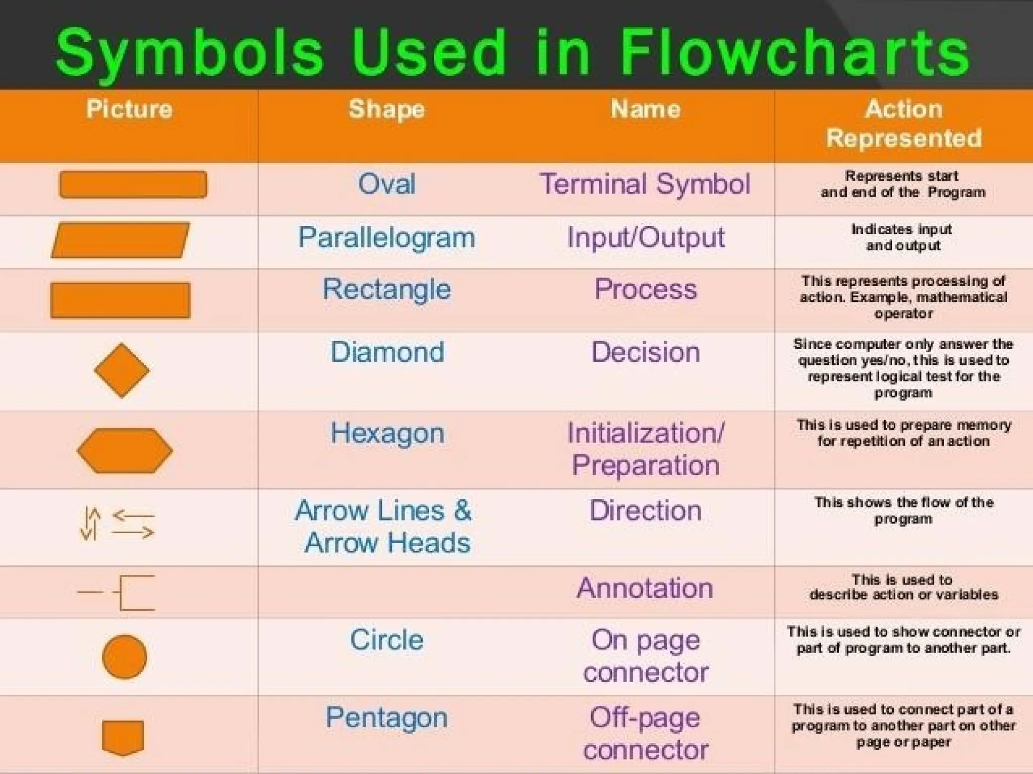
12. ALGORITHM DESIGN TOOL
• There can be two tools :
1. Flowchart
2. Pseudo Code
Flowchart :
“ Flowchart is graphical representation of the algorithms”
Pseudo Code :
“It is simply an implementation of an algorithm in the form
of annotations and informative text written in plain English.

13. FLOWCHART
Symbols used in Flowchart :

16. EXAMPLE OF FLOWCHART

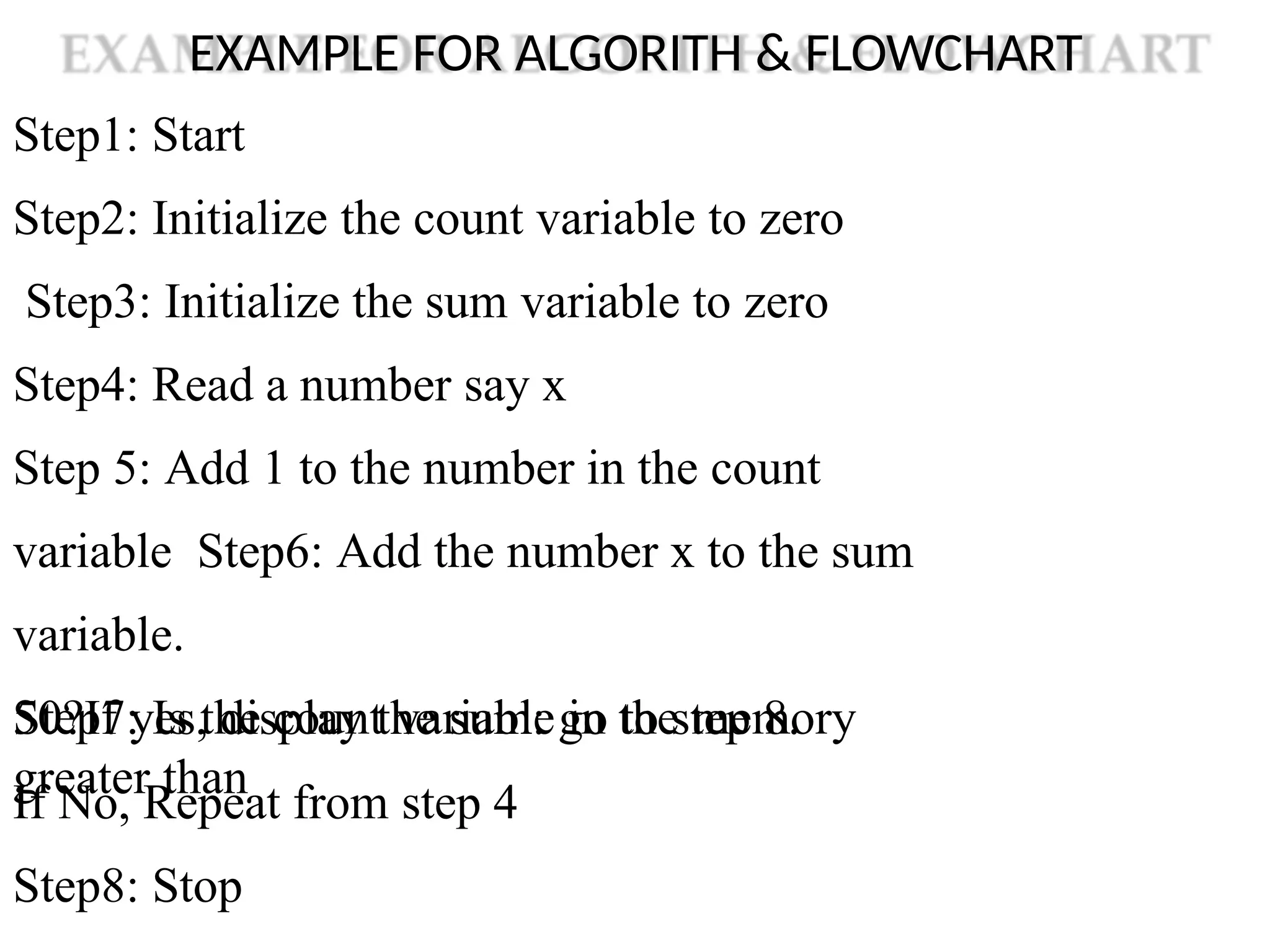
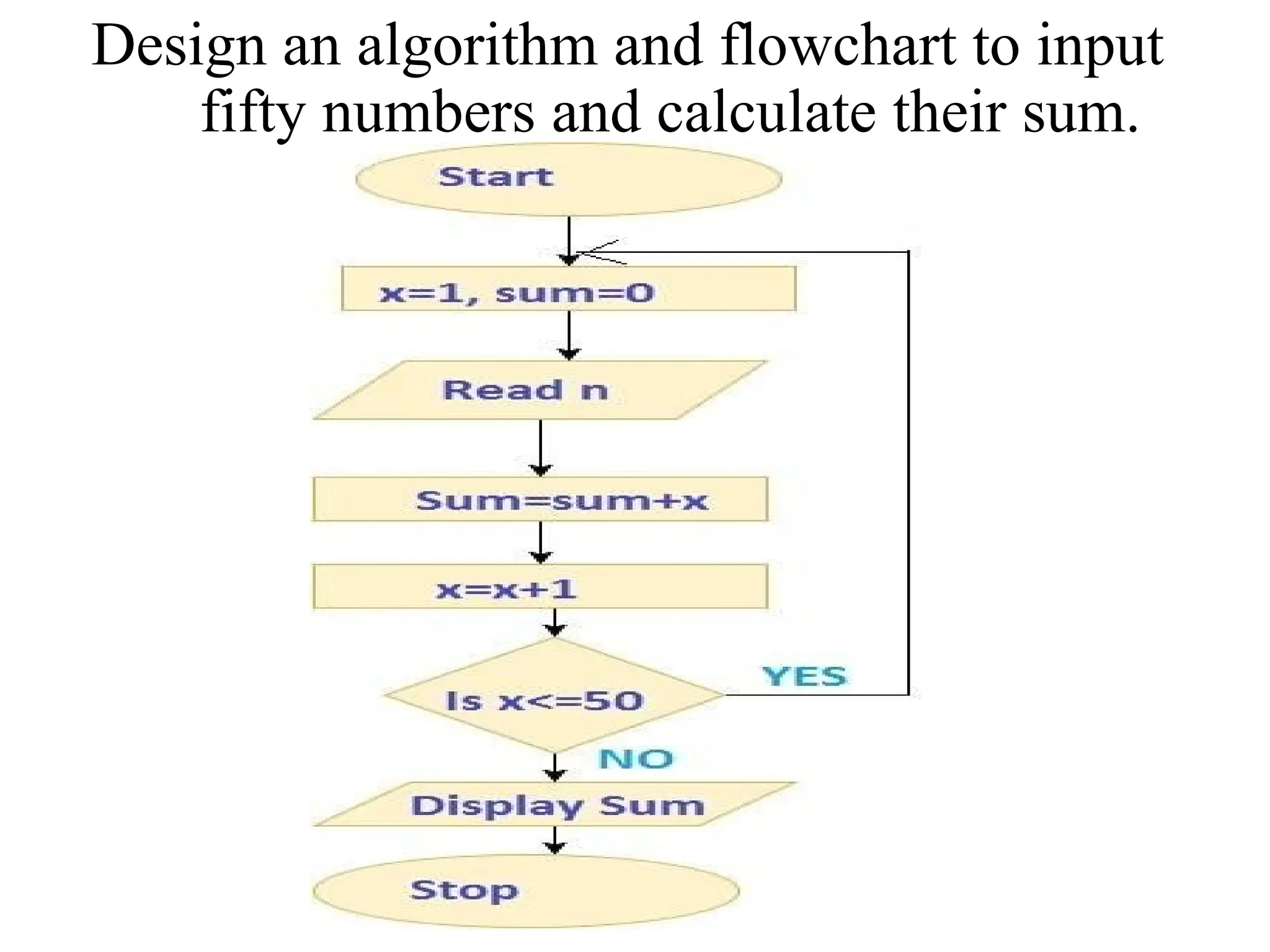
17. EXAMPLE FOR ALGORITH & FLOWCHART
Step1: Start
Step2: Initialize the count variable to zero
Step3: Initialize the sum variable to zero
Step4: Read a number say x
Step 5: Add 1 to the number in the count
variable Step6: Add the number x to the sum
variable.
Step7: Is the count variable in the memory
greater than
50?If yes, display the sum: go to step 8.
If No, Repeat from step 4
Step8: Stop

18. Design an algorithm and flowchart to input
fifty numbers and calculate their sum.

19. WRITE A PROGRAM FOR ADDING 10 NUMBERS

20. WRITE A PROGRAM TO FIND FACTORIAL OF NUMBER

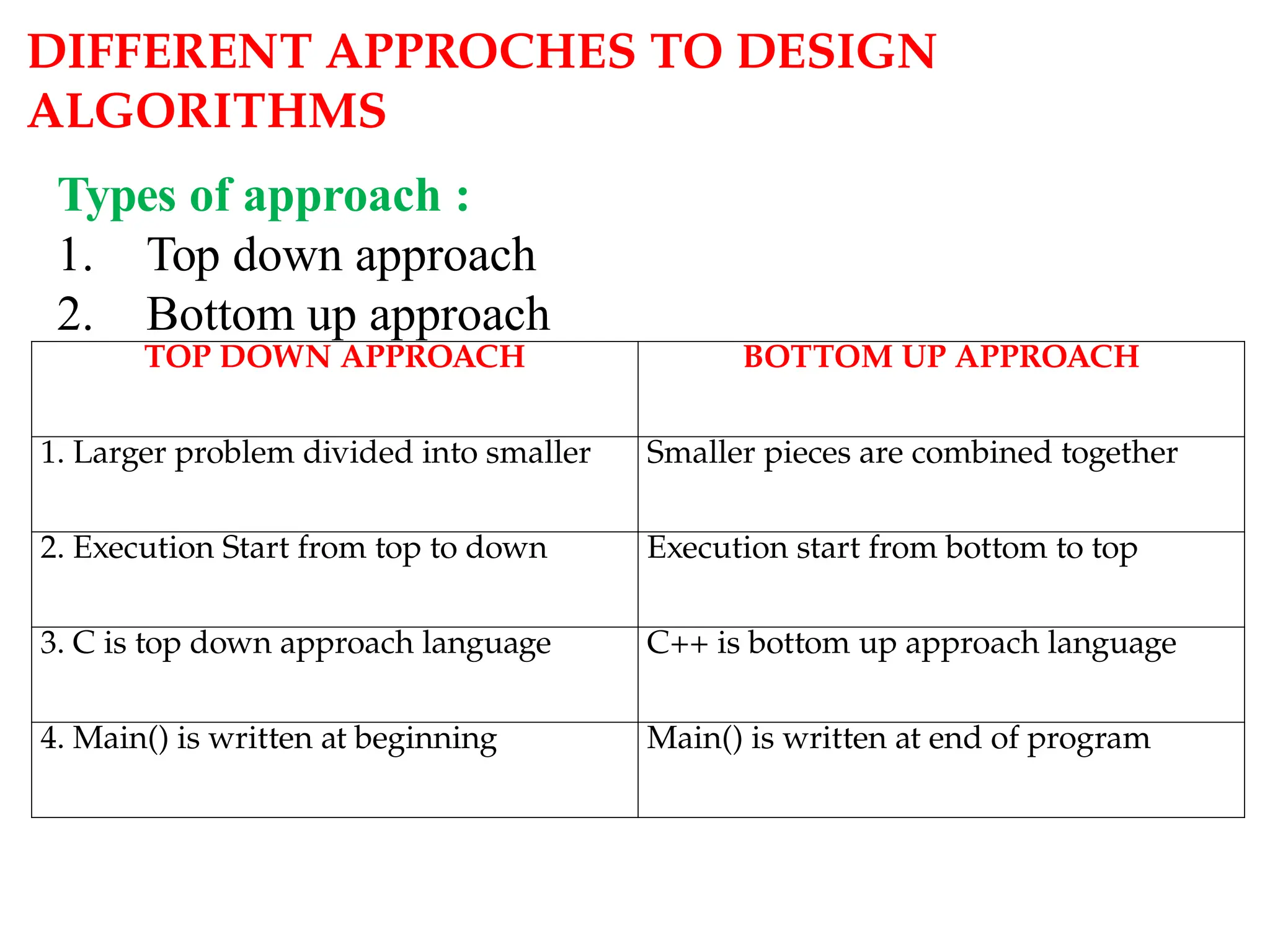
21. DIFFERENT APPROCHES TO DESIGN
ALGORITHMS
Types of approach :
1. Top down approach
2. Bottom up approach
TOP DOWN APPROACH BOTTOM UP APPROACH
1. Larger problem divided into smaller Smaller pieces are combined together
2. Execution Start from top to down Execution start from bottom to top
3. C is top down approach language C++ is bottom up approach language
4. Main() is written at beginning Main() is written at end of program

22. ALGORITHM ANALYSIS
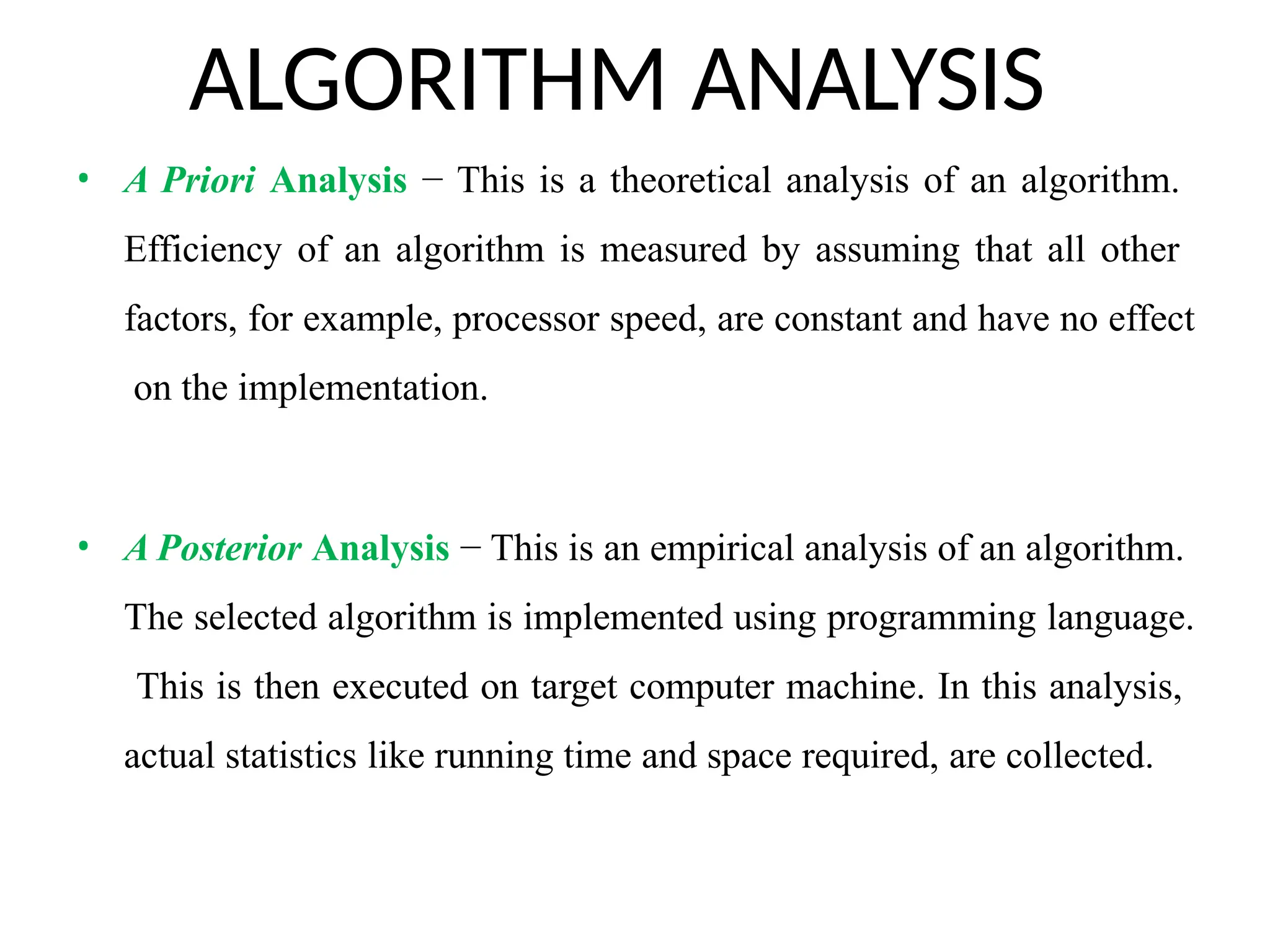
• A Priori Analysis − This is a theoretical analysis of an algorithm.
Efficiency of an algorithm is measured by assuming that all other
factors, for example, processor speed, are constant and have no effect
on the implementation.
• A Posterior Analysis − This is an empirical analysis of an algorithm.
The selected algorithm is implemented using programming language.
This is then executed on target computer machine. In this analysis,
actual statistics like running time and space required, are collected.

23. CASES OF ANALYSIS ALGORITHMS
.
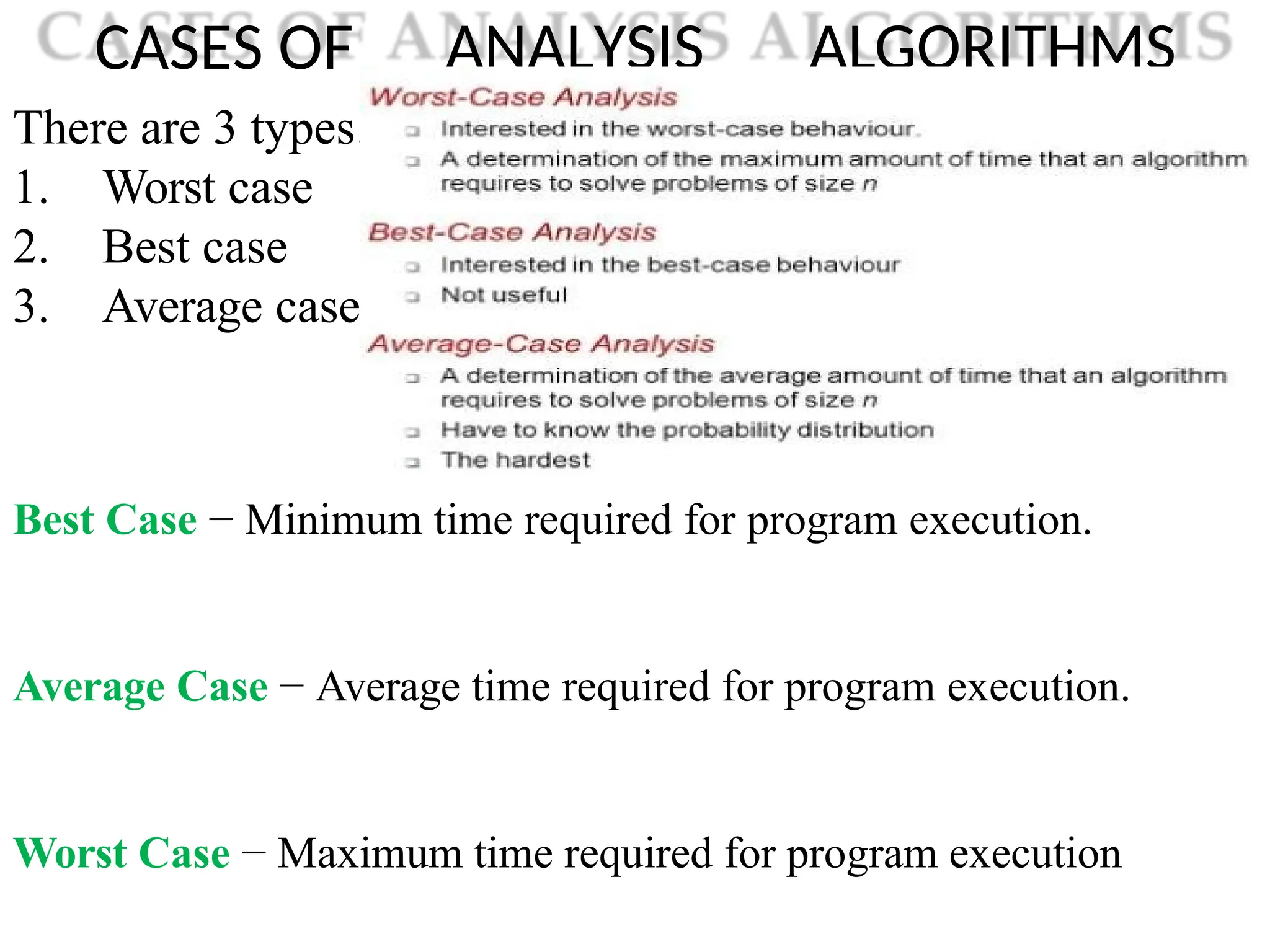
There are 3 types
1. Worst case
2. Best case
3. Average case
Best Case − Minimum time required for program execution.
Average Case − Average time required for program execution.
Worst Case − Maximum time required for program execution

24. Standard measure of efficiency
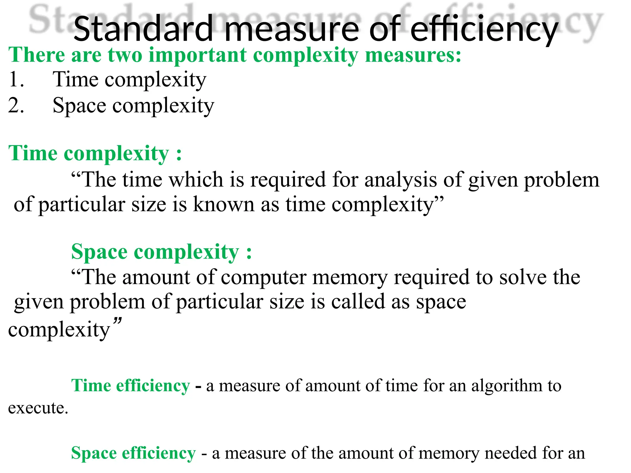
There are two important complexity measures:
1. Time complexity
2. Space complexity
Time complexity :
“The time which is required for analysis of given problem
of particular size is known as time complexity”
Space complexity :
“The amount of computer memory required to solve the
given problem of particular size is called as space
complexity”
Time efficiency - a measure of amount of time for an algorithm to
execute.
Space efficiency - a measure of the amount of memory needed for an

26. DATA TYPES IN C++

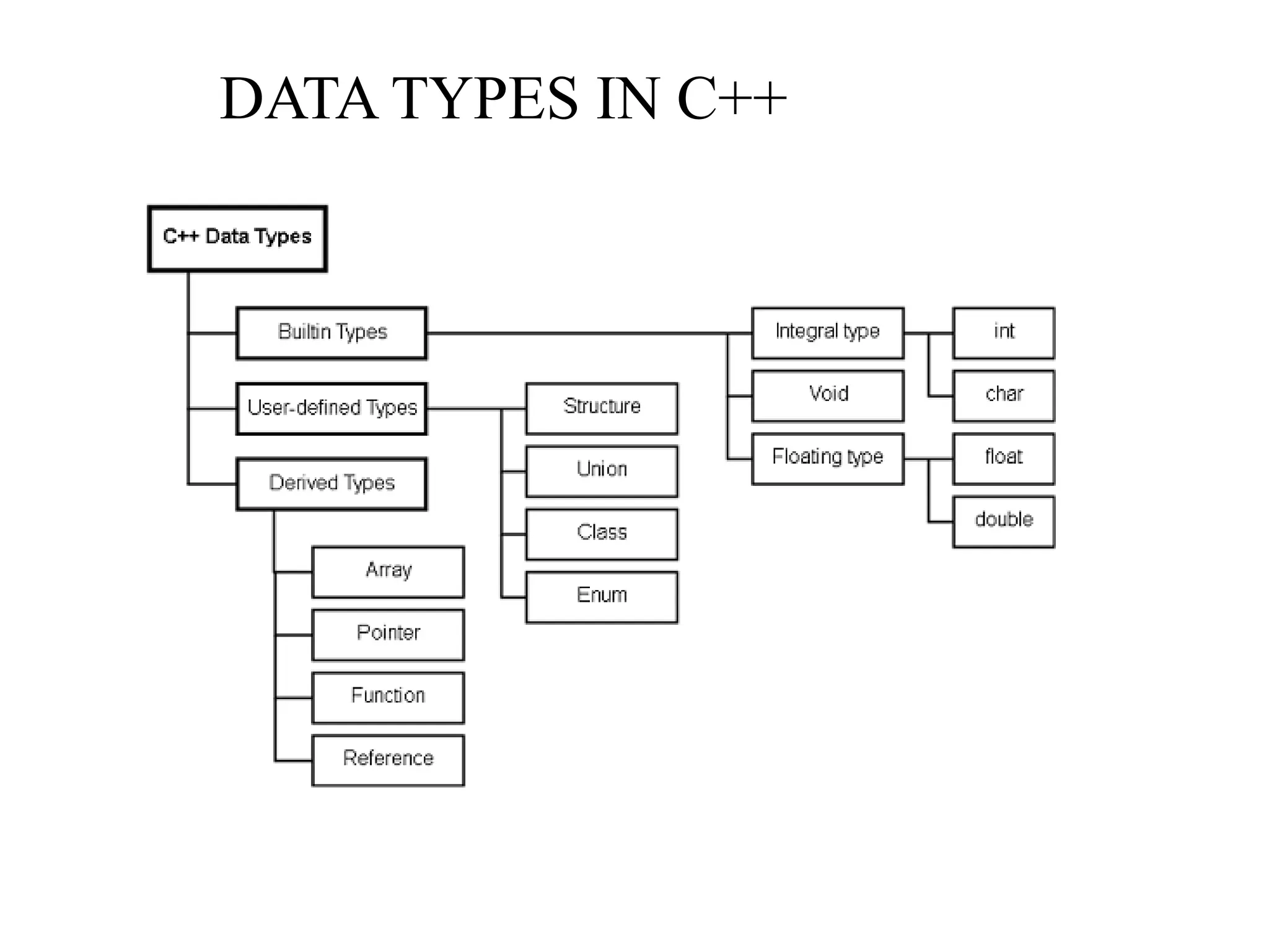
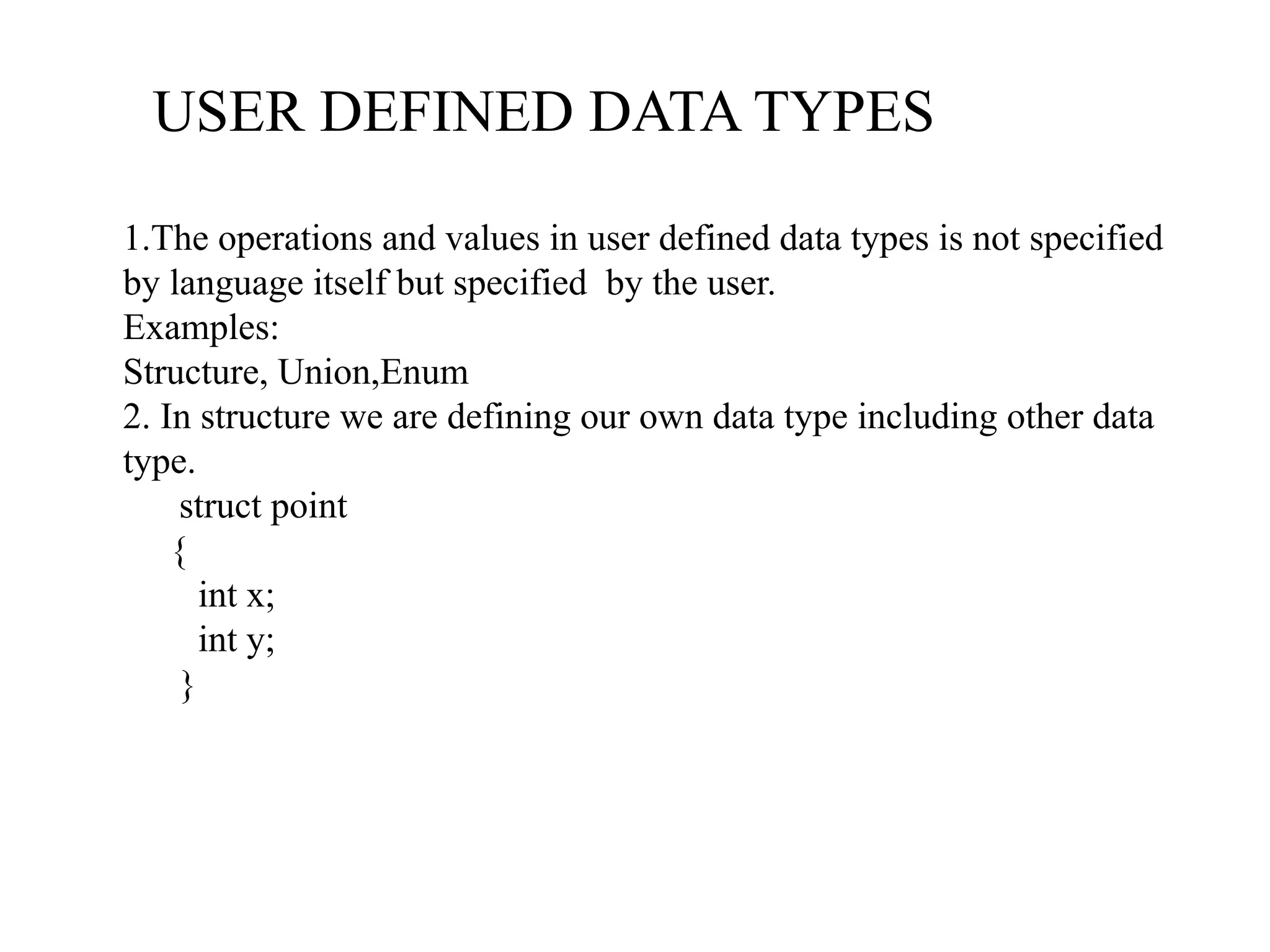
27. USER DEFINED DATA TYPES
1.The operations and values in user defined data types is not specified
by language itself but specified by the user.
Examples:
Structure, Union,Enum
2. In structure we are defining our own data type including other data
type.
struct point
{
int x;
int y;
}

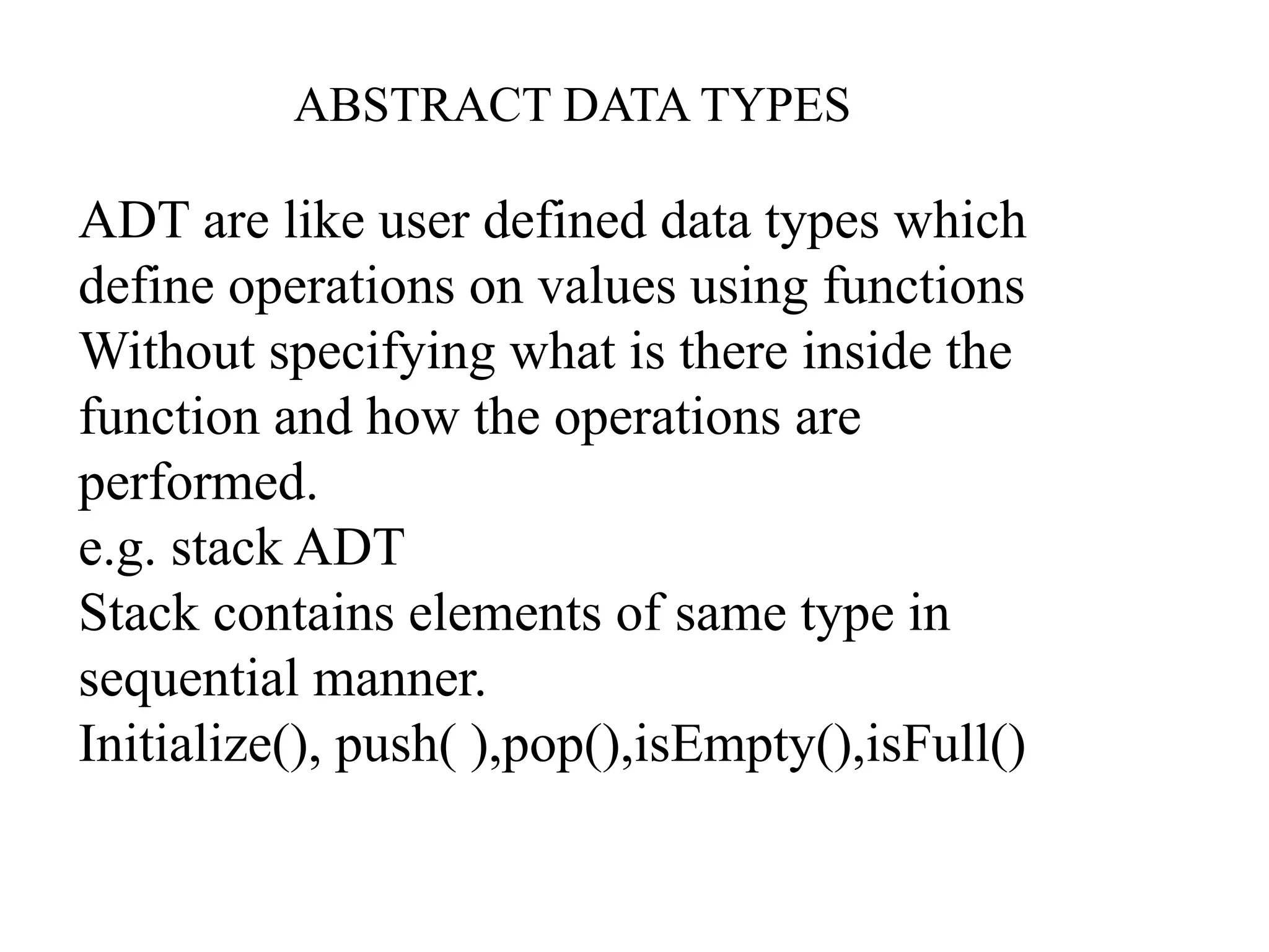
28. ABSTRACT DATA TYPES
ADT are like user defined data types which
define operations on values using functions
Without specifying what is there inside the
function and how the operations are
performed.
e.g. stack ADT
Stack contains elements of same type in
sequential manner.
Initialize(), push( ),pop(),isEmpty(),isFull()

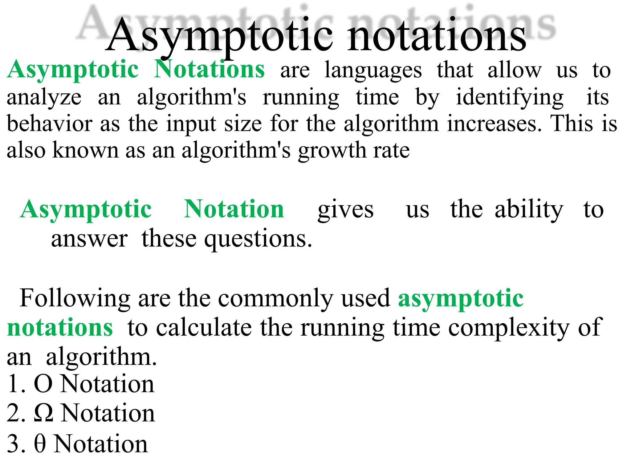
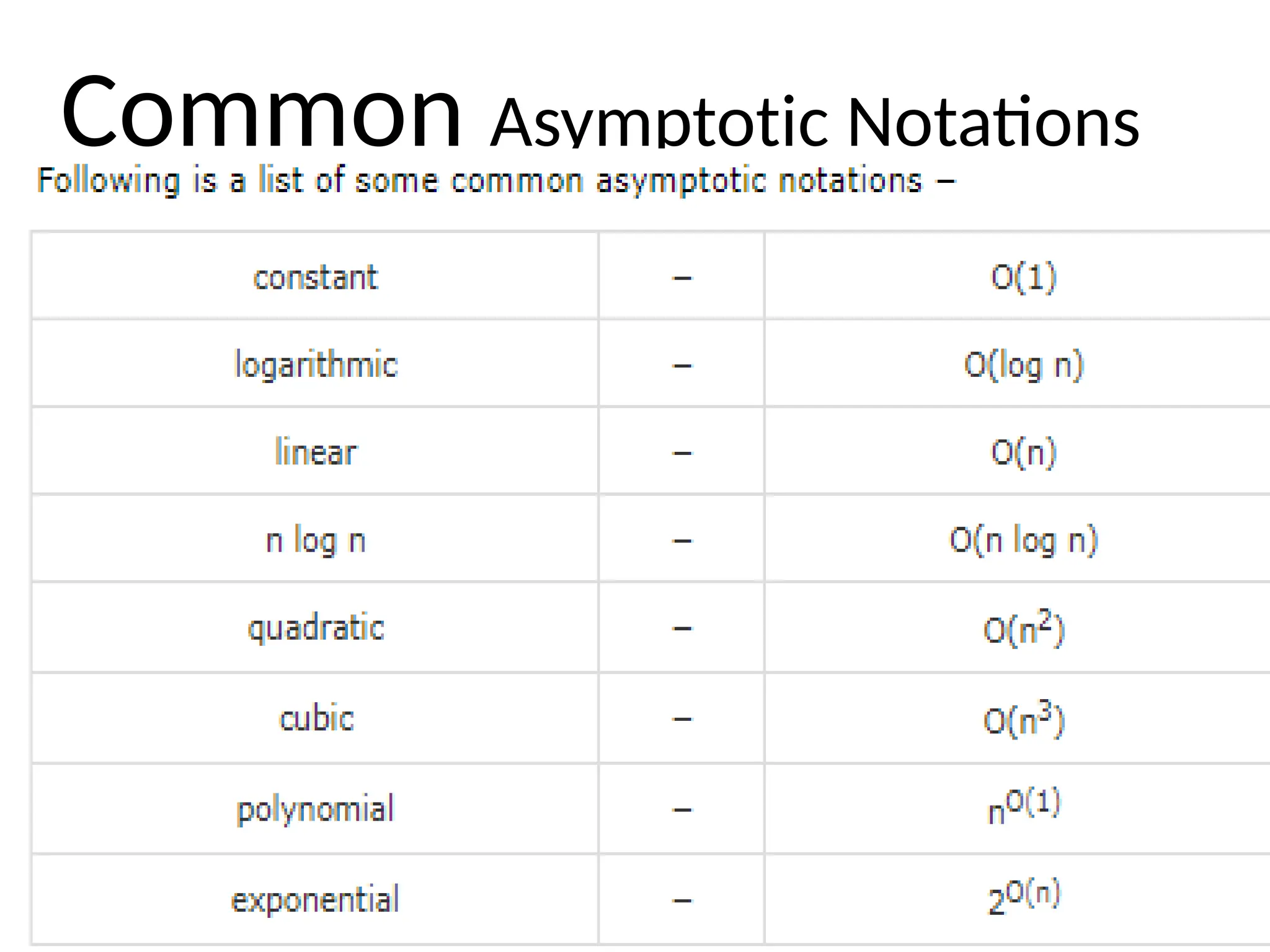
29. Asymptotic notations
Asymptotic Notations are languages that allow us to
analyze an algorithm's running time by identifying its
behavior as the input size for the algorithm increases. This is
also known as an algorithm's growth rate
Asymptotic Notation gives us the ability to
answer these questions.
Following are the commonly used asymptotic
notations to calculate the running time complexity of
an algorithm.
1. Ο Notation
2. Ω Notation
3. θ Notation

30. n 5n2
6n 12
1 21.74% 26.09% 52.17%
10 87.41% 10.49% 2.09%
100 98.79% 1.19% 0.02%
1000 99.88% 0.12% 0.0002%
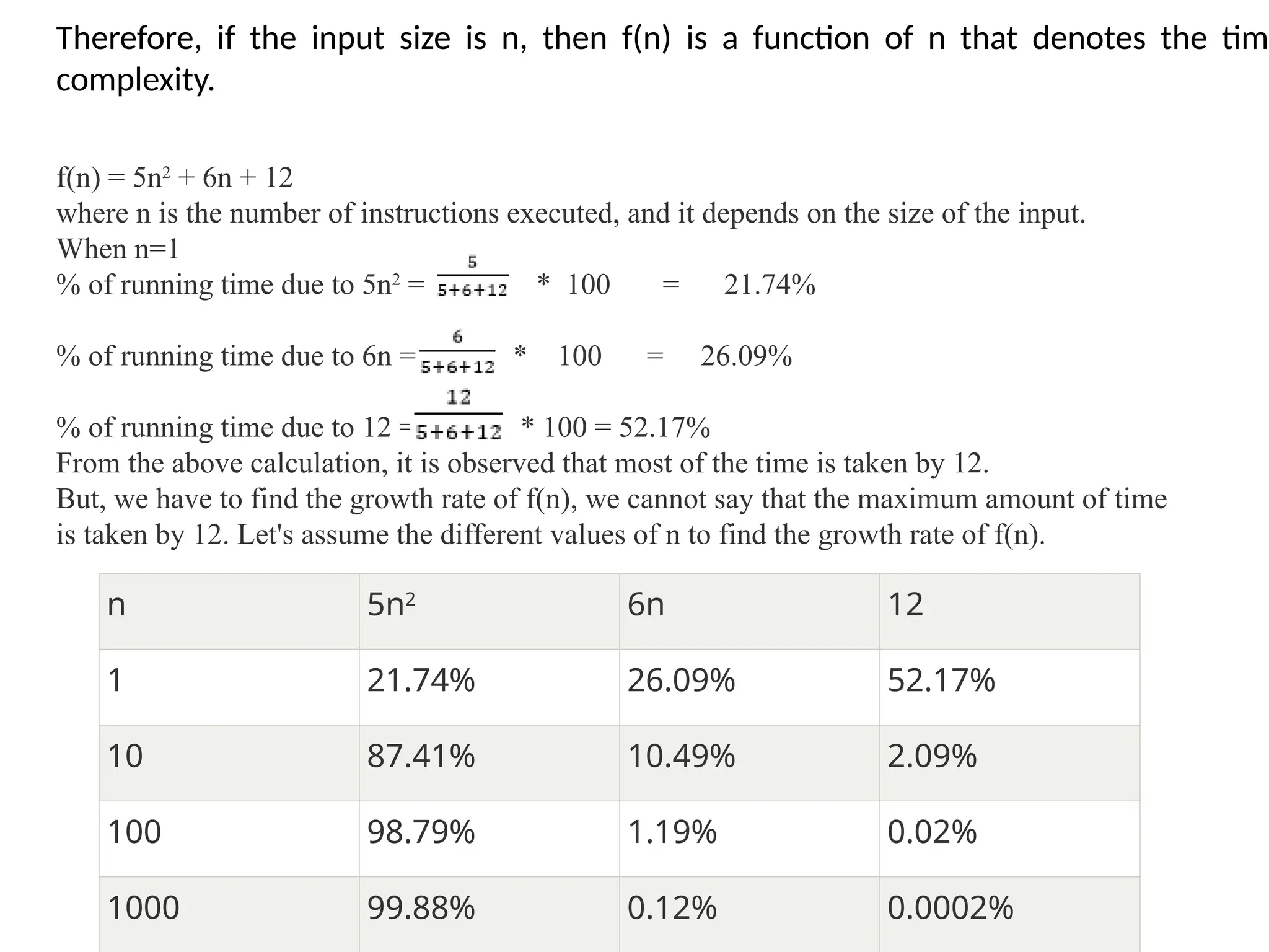
Therefore, if the input size is n, then f(n) is a function of n that denotes the time
complexity.
f(n) = 5n2
+ 6n + 12
where n is the number of instructions executed, and it depends on the size of the input.
When n=1
% of running time due to 5n2
= * 100 = 21.74%
% of running time due to 6n = * 100 = 26.09%
% of running time due to 12 = * 100 = 52.17%
From the above calculation, it is observed that most of the time is taken by 12.
But, we have to find the growth rate of f(n), we cannot say that the maximum amount of time
is taken by 12. Let's assume the different values of n to find the growth rate of f(n).

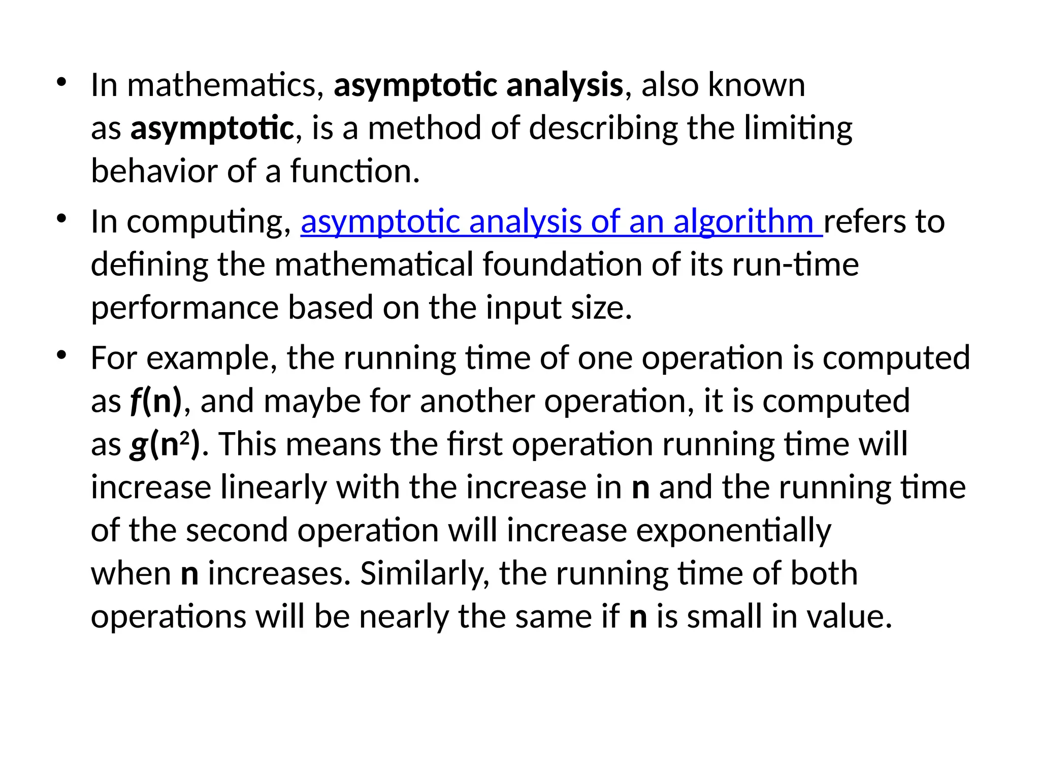
31. • In mathematics, asymptotic analysis, also known
as asymptotic, is a method of describing the limiting
behavior of a function.
• In computing, asymptotic analysis of an algorithm refers to
defining the mathematical foundation of its run-time
performance based on the input size.
• For example, the running time of one operation is computed
as f(n), and maybe for another operation, it is computed
as g(n2
). This means the first operation running time will
increase linearly with the increase in n and the running time
of the second operation will increase exponentially
when n increases. Similarly, the running time of both
operations will be nearly the same if n is small in value.

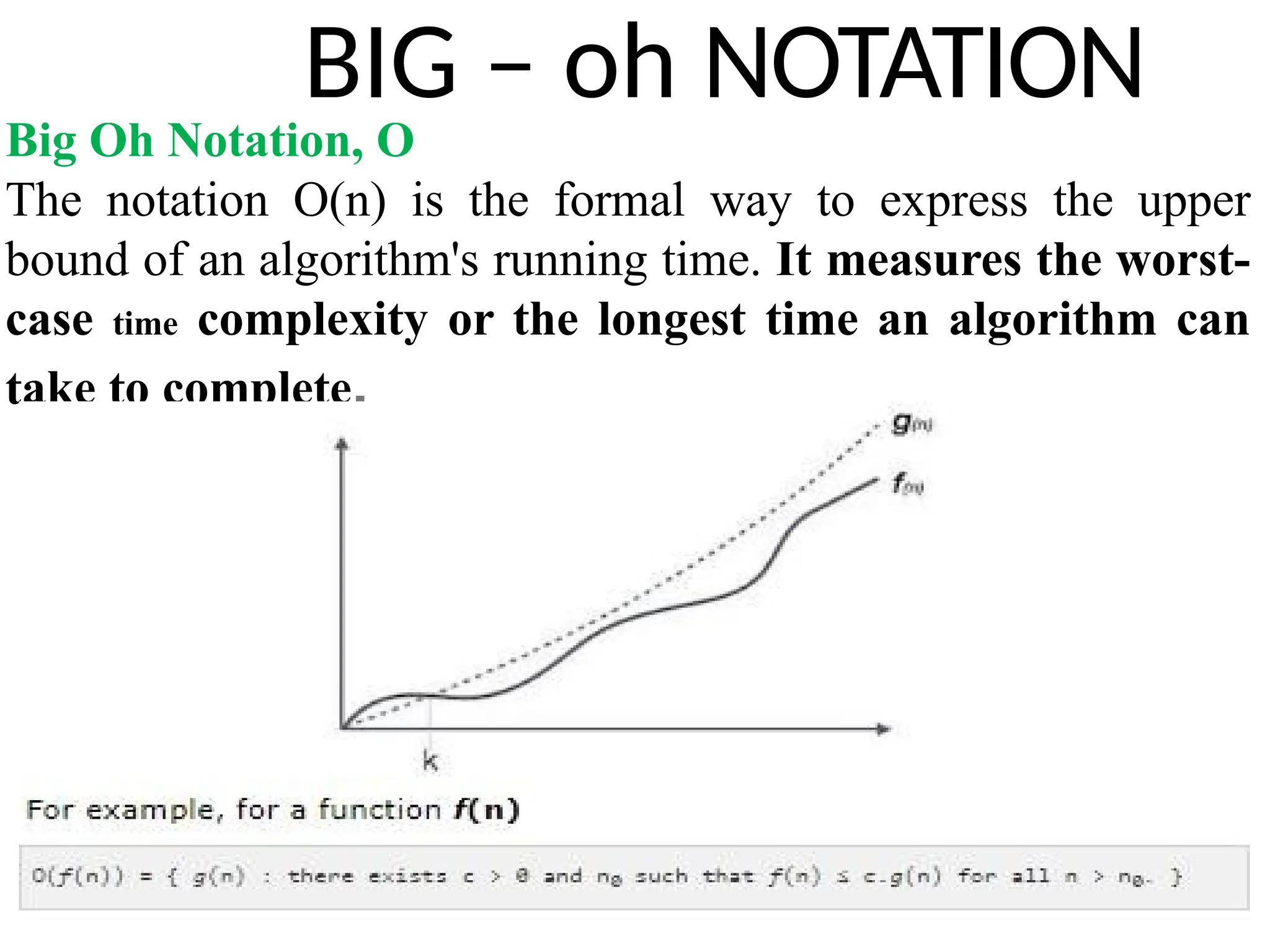
32. BIG – oh NOTATION
Big Oh Notation, Ο
The notation Ο(n) is the formal way to express the upper
bound of an algorithm's running time. It measures the worst-
case time complexity or the longest time an algorithm can
take to complete.

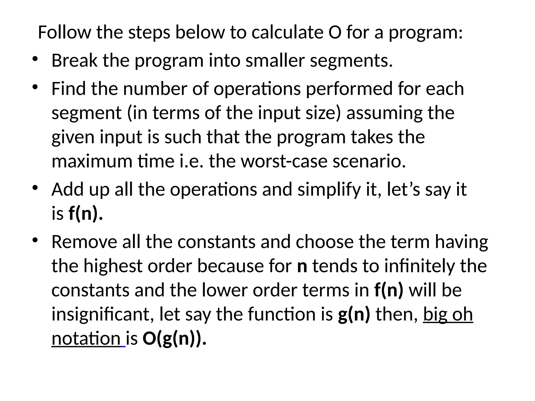
33. Follow the steps below to calculate O for a program:
• Break the program into smaller segments.
• Find the number of operations performed for each
segment (in terms of the input size) assuming the
given input is such that the program takes the
maximum time i.e. the worst-case scenario.
• Add up all the operations and simplify it, let’s say it
is f(n).
• Remove all the constants and choose the term having
the highest order because for n tends to infinitely the
constants and the lower order terms in f(n) will be
insignificant, let say the function is g(n) then, big oh
notation is O(g(n)).

34. Omega NOTATION
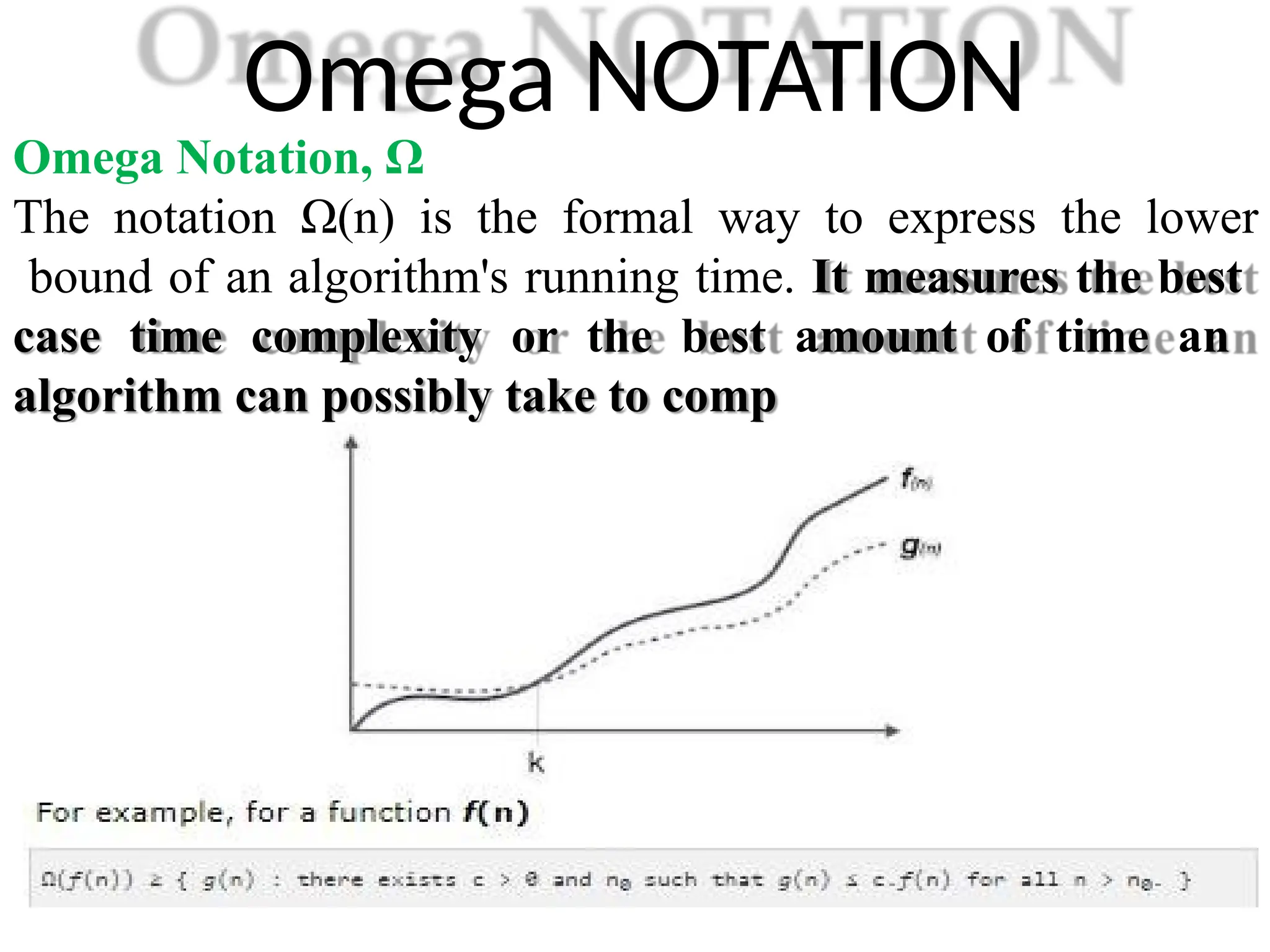
Omega Notation, Ω
The notation Ω(n) is the formal way to express the lower
bound of an algorithm's running time. It measures the best
case time complexity or the best amount of time an
algorithm can possibly take to comp

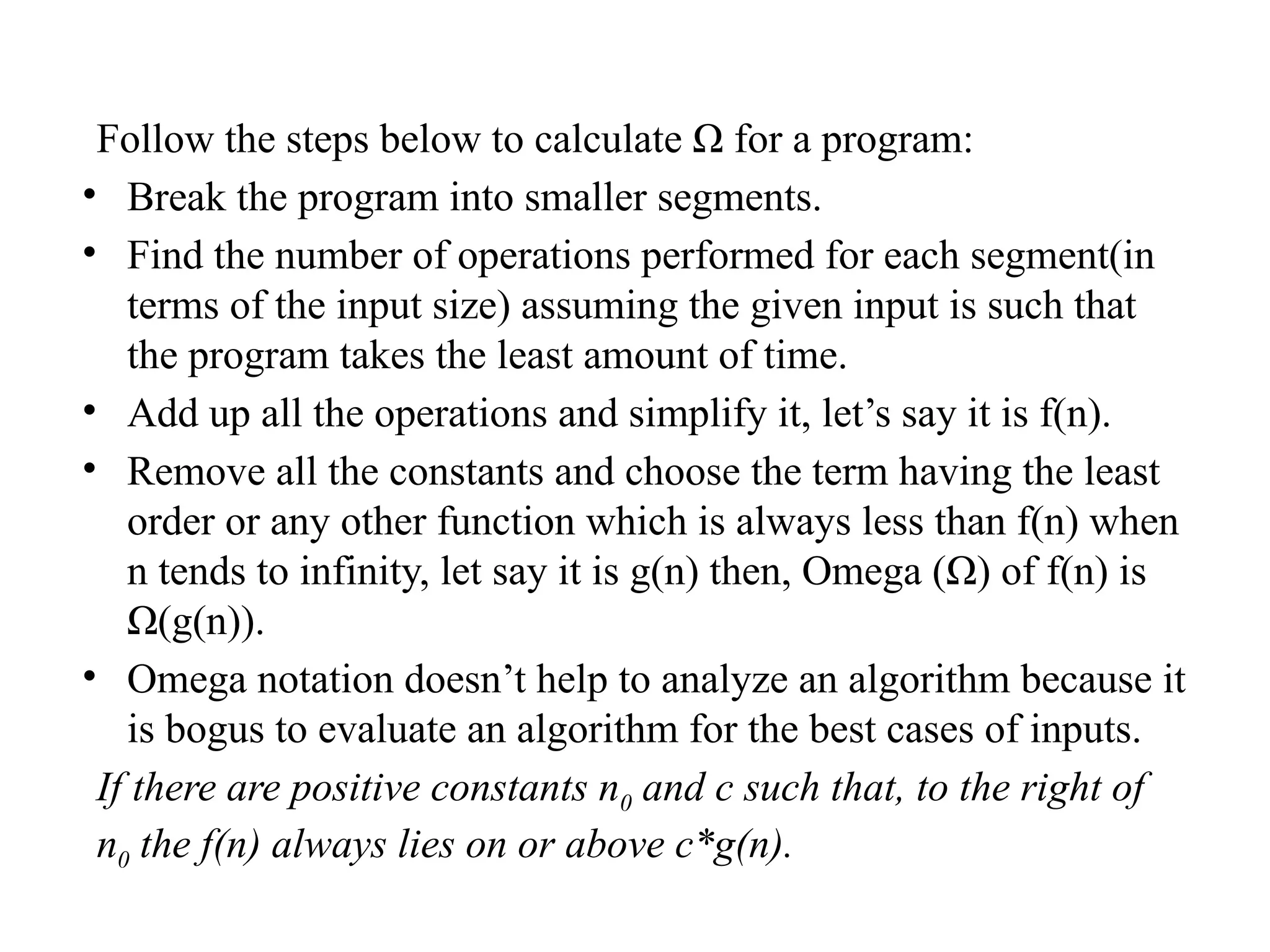
35. Follow the steps below to calculate Ω for a program:
• Break the program into smaller segments.
• Find the number of operations performed for each segment(in
terms of the input size) assuming the given input is such that
the program takes the least amount of time.
• Add up all the operations and simplify it, let’s say it is f(n).
• Remove all the constants and choose the term having the least
order or any other function which is always less than f(n) when
n tends to infinity, let say it is g(n) then, Omega (Ω) of f(n) is
Ω(g(n)).
• Omega notation doesn’t help to analyze an algorithm because it
is bogus to evaluate an algorithm for the best cases of inputs.
If there are positive constants n0 and c such that, to the right of
n0 the f(n) always lies on or above c*g(n).

36. Theta NOTATION
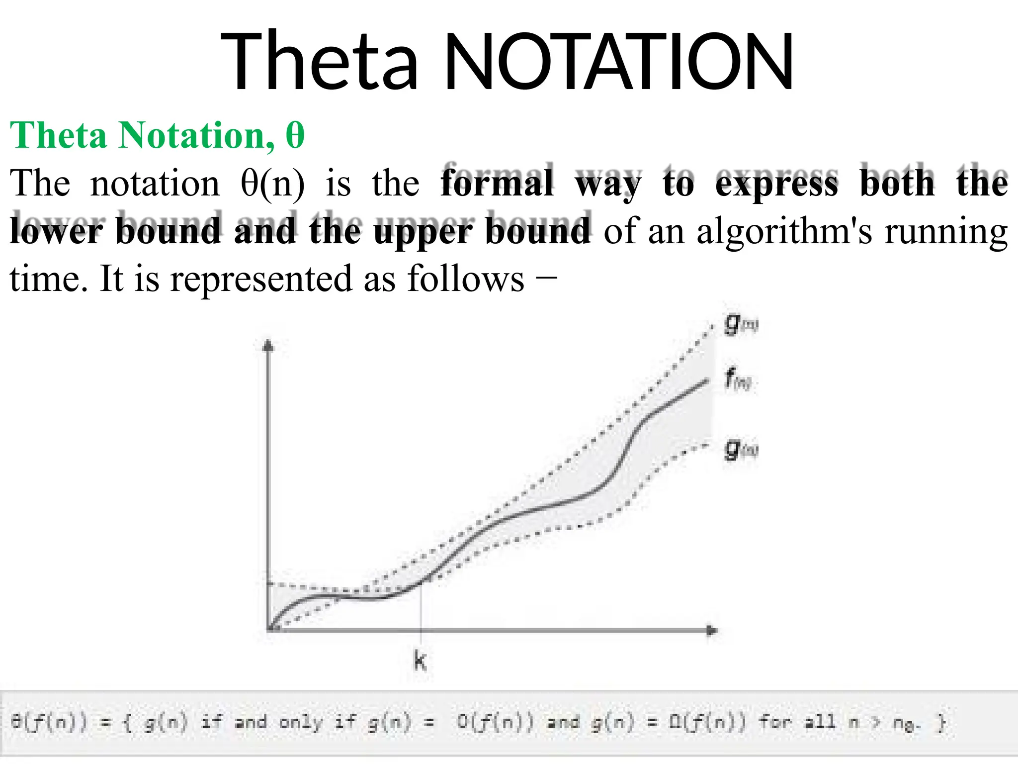
Theta Notation, θ
The notation θ(n) is the formal way to express both the
lower bound and the upper bound of an algorithm's running
time. It is represented as follows −

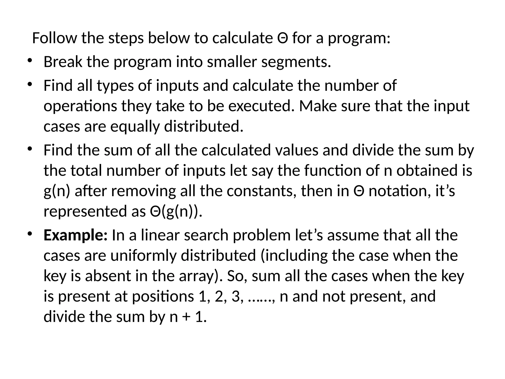
37. Follow the steps below to calculate Θ for a program:
• Break the program into smaller segments.
• Find all types of inputs and calculate the number of
operations they take to be executed. Make sure that the input
cases are equally distributed.
• Find the sum of all the calculated values and divide the sum by
the total number of inputs let say the function of n obtained is
g(n) after removing all the constants, then in Θ notation, it’s
represented as Θ(g(n)).
• Example: In a linear search problem let’s assume that all the
cases are uniformly distributed (including the case when the
key is absent in the array). So, sum all the cases when the key
is present at positions 1, 2, 3, ……, n and not present, and
divide the sum by n + 1.

38. Common Asymptotic Notations

39. DATA
STRUCTURE

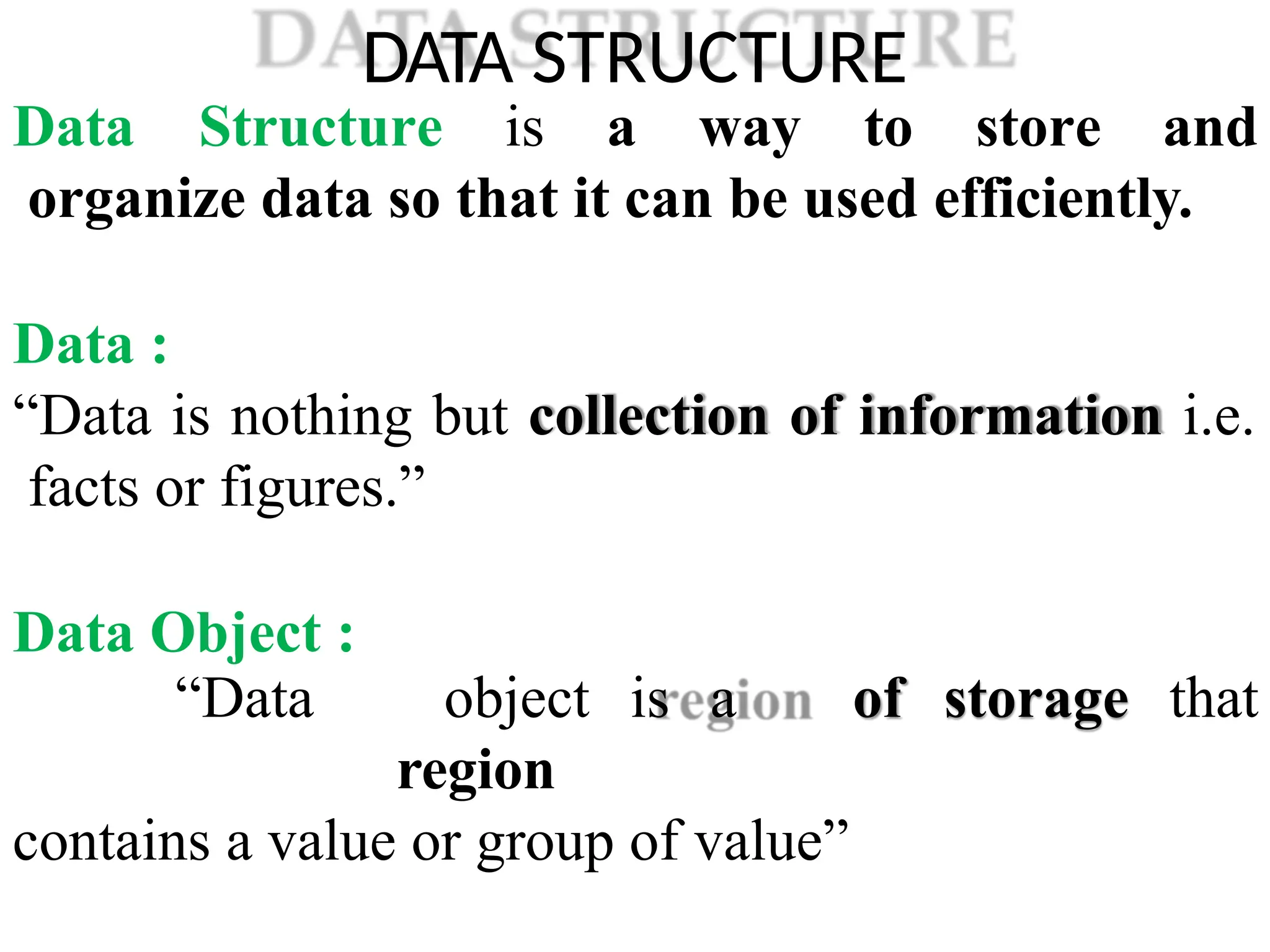
40. DATA STRUCTURE
Data Structure is a way to store and
organize data so that it can be used efficiently.
Data :
“Data is nothing but collection of information i.e.
facts or figures.”
Data Object :
of storage that
“Data object is a
region
contains a value or group of value”

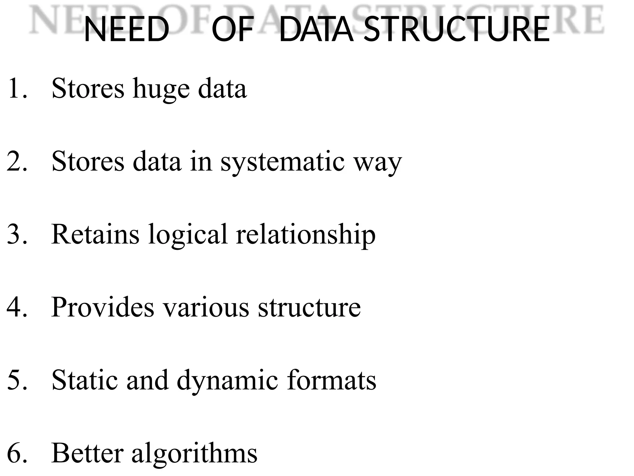
41. NEED OF DATA STRUCTURE
1. Stores huge data
2. Stores data in systematic way
3. Retains logical relationship
4. Provides various structure
5. Static and dynamic formats
6. Better algorithms

42. ABSTRACT DATA TYPE
ADT :
“Abstract data types are mathematical models of a set of data
values or information that share similar behavior or qualities and that can
be specified and identified independent of specific implementations.
Abstract data types, or ADTs, are typically used in algorithms.”
Another definition
of ADT is ADT is set of D,
F and A.
D – domain = Data
object
F – function = set of operations which can carried out on data

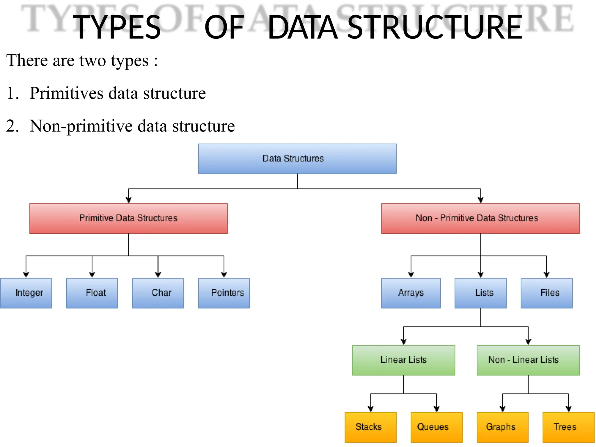
43. TYPES OF DATA STRUCTURE
There are two types :
1. Primitives data structure
2. Non-primitive data structure

44. TYPES OF DATA STRUCTURE
1. Primitives data structure :
“Primitive data structures are those which are predefined
way of storing data by the system. ”
e.g. int, char, float etc
2. Non-primitive data structure :
“The data types that are derived from primary data types are known as
non-Primitive data types. These datatype are used to store group of values.”
e.g. struct, array, linklist, stack, tree , graph etc.

45. Linear and Non-Linear Data
Structure
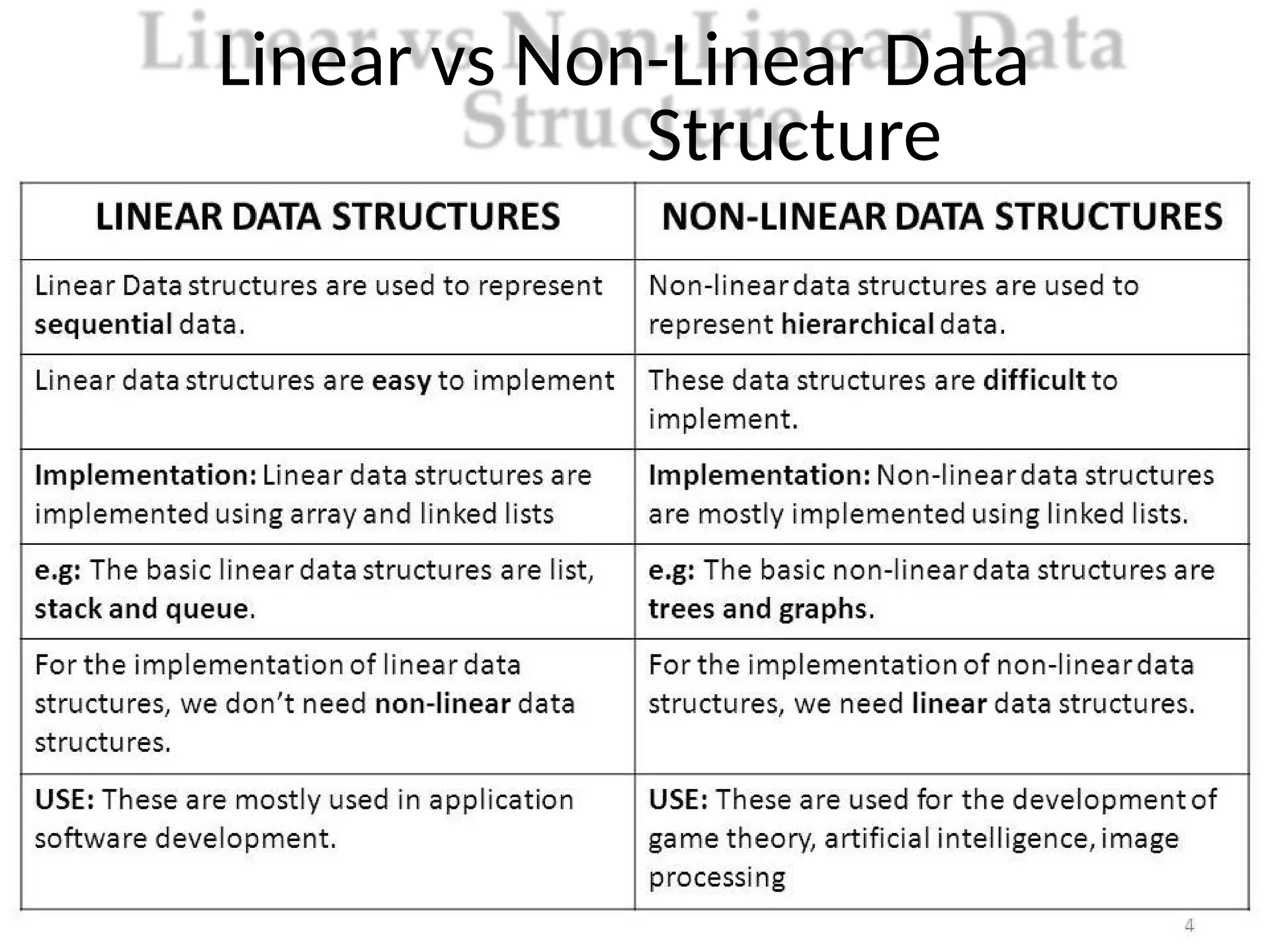
1. Linear Data Strucute :
“Linear data structuretraverses the data elements
sequentially, in which only one data element can directly be
reached”
Ex: Arrays, Linked Lists, stack, queue.
2. Non-Linear Data Strucute :
“Every data item is attached to several other data items in a
way that is specific for reflecting relationships.”
Ex: Graph, Tree

46. Linear vs Non-Linear Data
Structure

47. Static and Dynamic
Data Structure
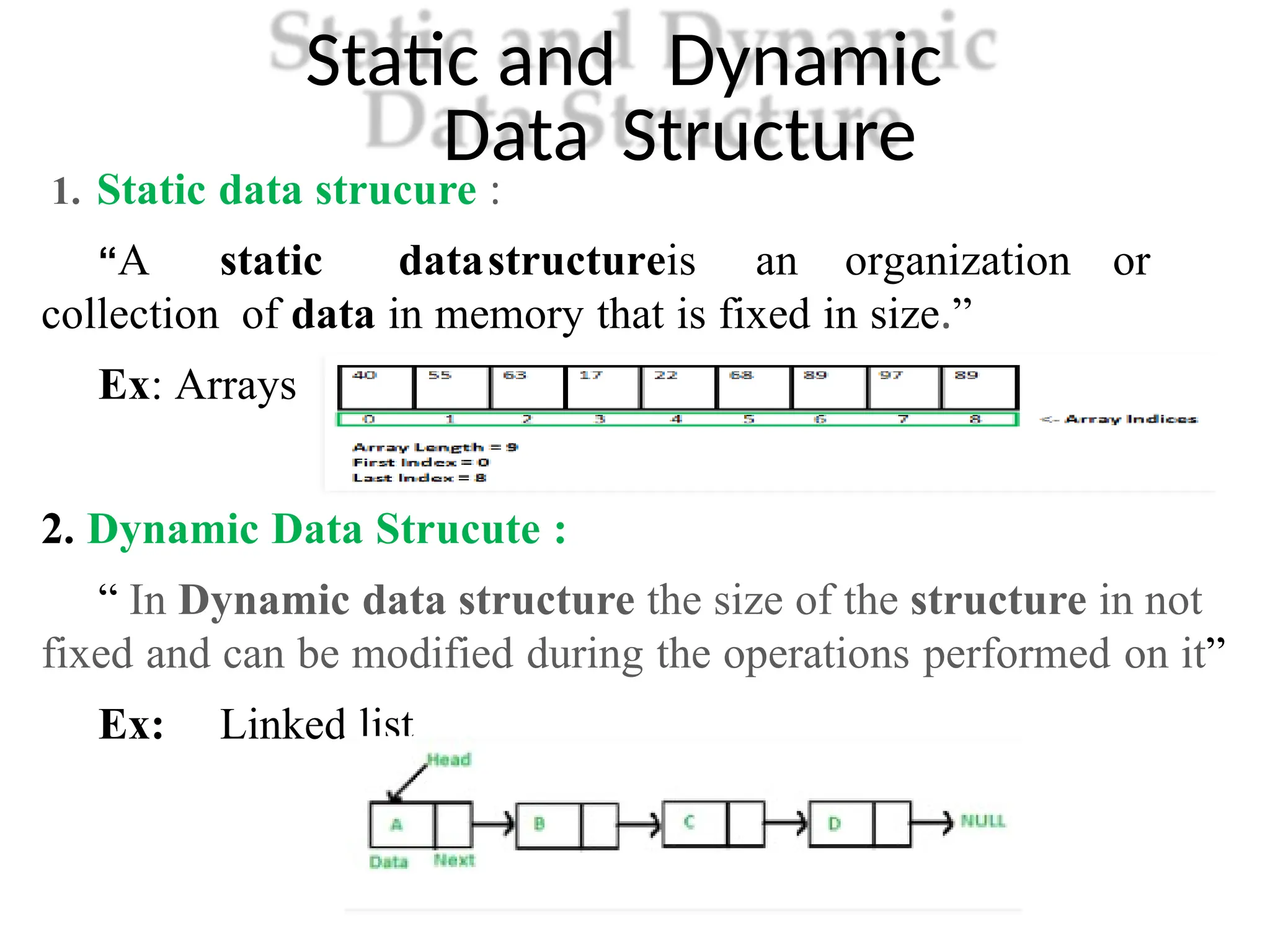
1. Static data strucure :
“A static datastructureis an organization or
collection of data in memory that is fixed in size.”
Ex: Arrays
2. Dynamic Data Strucute :
“ In Dynamic data structure the size of the structure in not
fixed and can be modified during the operations performed on it”
Ex: Linked list

48. Persistent and Ephemeral
Data Structure
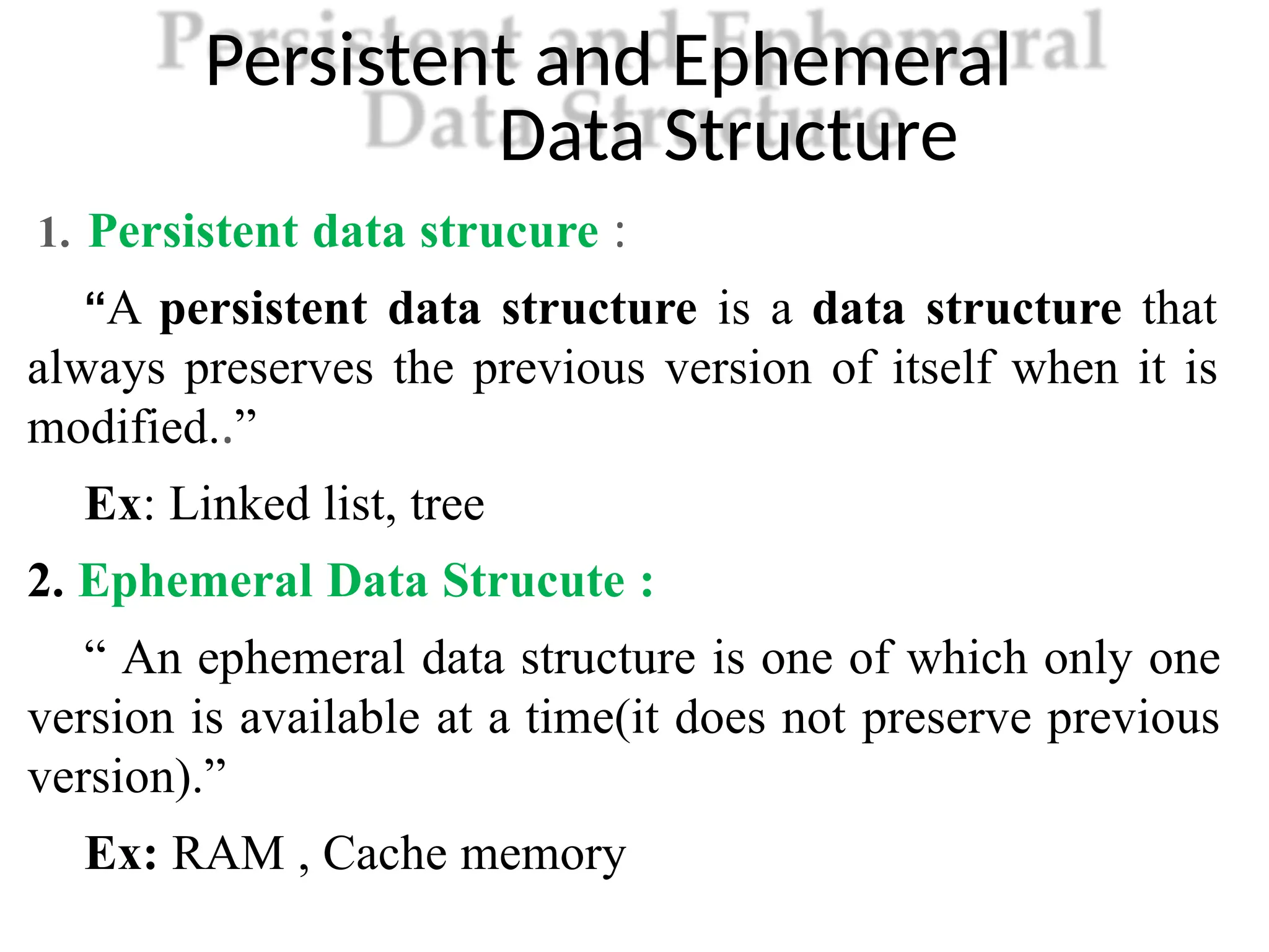
1. Persistent data strucure :
“A persistent data structure is a data structure that
always preserves the previous version of itself when it is
modified..”
Ex: Linked list, tree
2. Ephemeral Data Strucute :
“ An ephemeral data structure is one of which only one
version is available at a time(it does not preserve previous
version).”
Ex: RAM , Cache memory

49. Relationship among Data, Data
Structure and Algorithms
Data is considered as set of facts and figures or data is value of
group of value which is in particular format.
Data structure is method of gathering as well as organizing data
in such manner that several operation can be performed
Problem is defined as a situation or condition which need
to solve to achieve the goals
Algorithm is set of ordered instruction which are written
in simple english language.

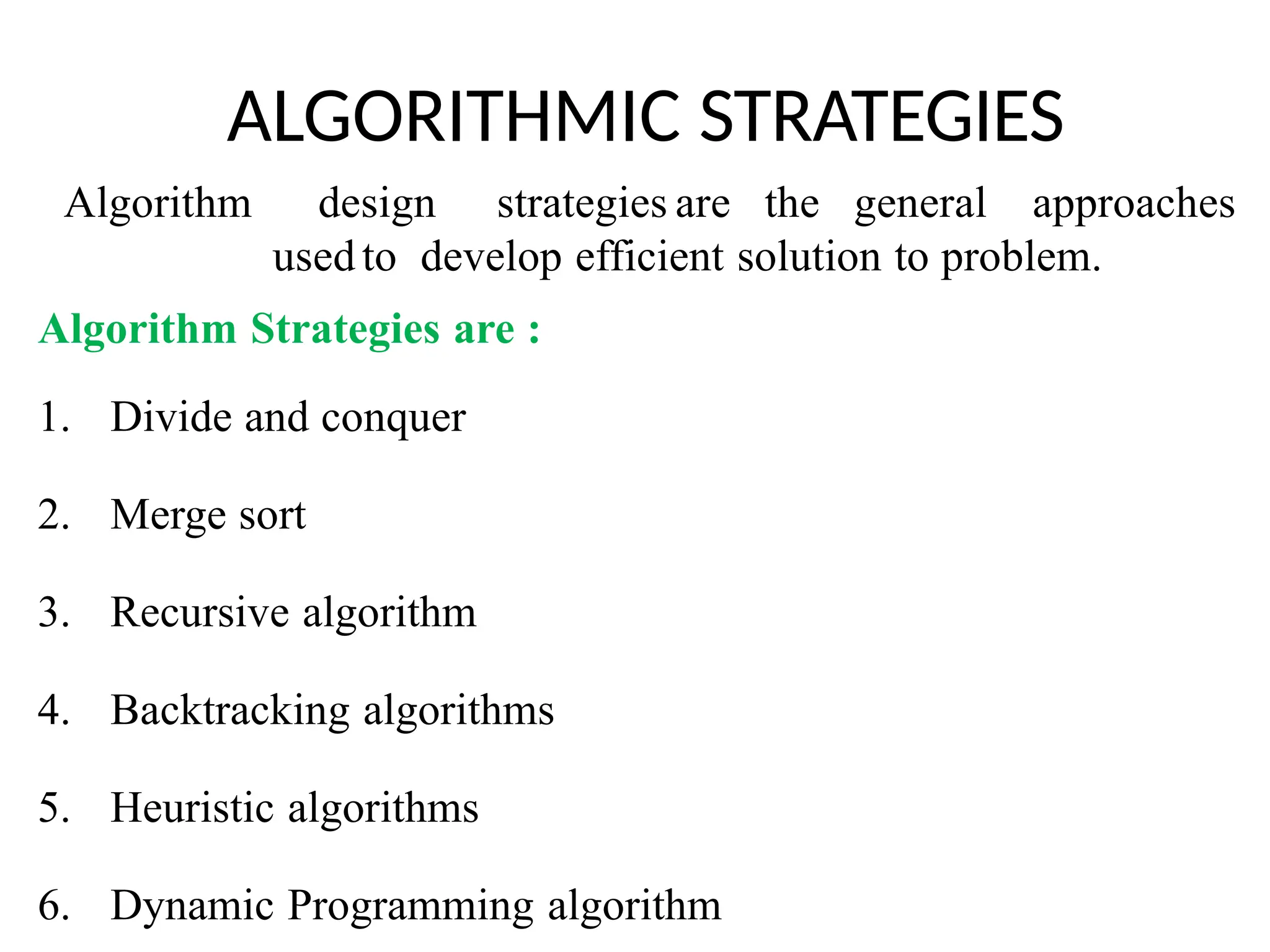
50. ALGORITHMIC STRATEGIES
Algorithm design strategies are the general approaches
usedto develop efficient solution to problem.
Algorithm Strategies are :
1. Divide and conquer
2. Merge sort
3. Recursive algorithm
4. Backtracking algorithms
5. Heuristic algorithms
6. Dynamic Programming algorithm

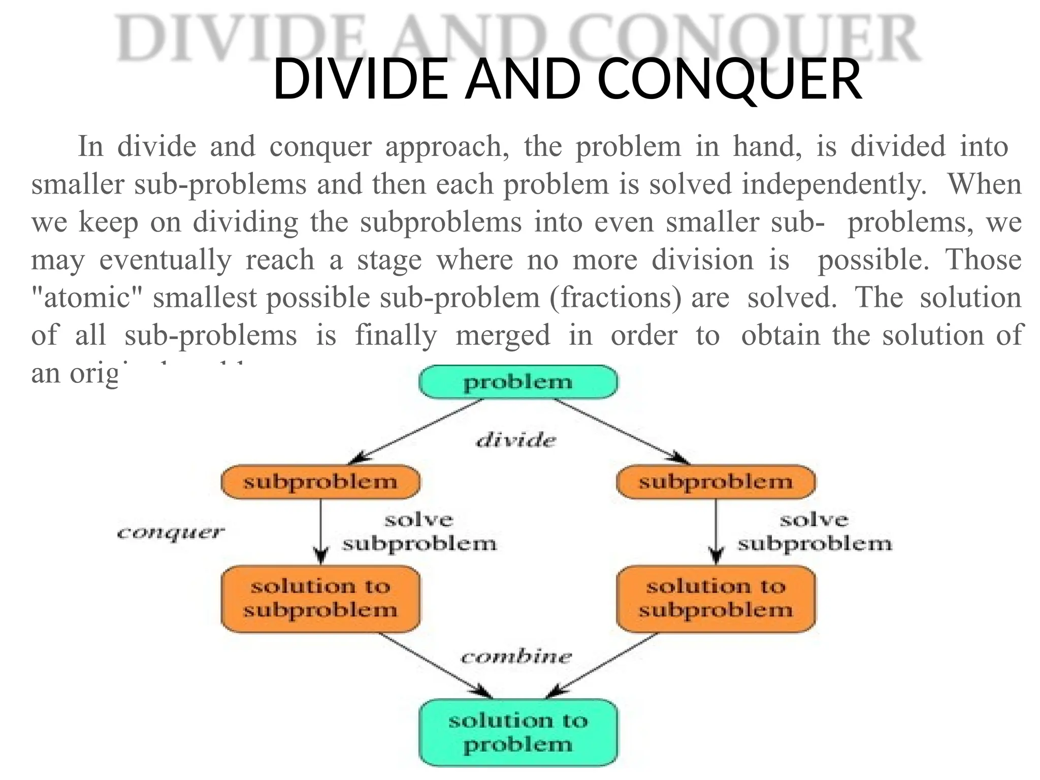
51. DIVIDE AND CONQUER
In divide and conquer approach, the problem in hand, is divided into
smaller sub-problems and then each problem is solved independently. When
we keep on dividing the subproblems into even smaller sub- problems, we
may eventually reach a stage where no more division is possible. Those
"atomic" smallest possible sub-problem (fractions) are solved. The solution
of all sub-problems is finally merged in order to obtain the solution of
an original problem.

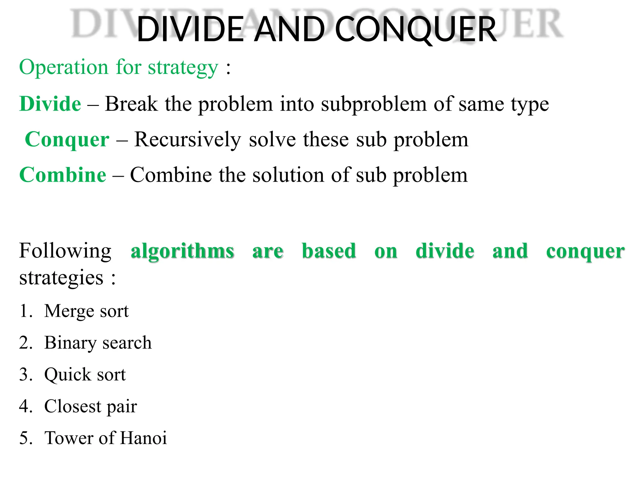
52. DIVIDE AND CONQUER
Operation for strategy :
Divide – Break the problem into subproblem of same type
Conquer – Recursively solve these sub problem
Combine – Combine the solution of sub problem
are based on divide and conquer
Following algorithms
strategies :
1. Merge sort
2. Binary search
3. Quick sort
4. Closest pair
5. Tower of Hanoi

53. DIVIDE AND CONQUER
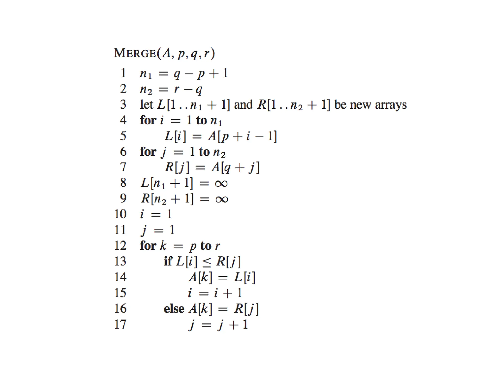
1. Merge sort :
Merge Sort is a divide-and-conquer algorithm. It divides the input array in
two halves, calls itself for the two halves and then merges the two sorted
halves. The merge() function is used for merging two halves. The
merge(arr, l, m, r) is key process that assumes that arr[l..m] and arr[m+1..r]
are sorted and merges the two sorted sub-arrays into one.

55. DIVIDE AND CONQUER
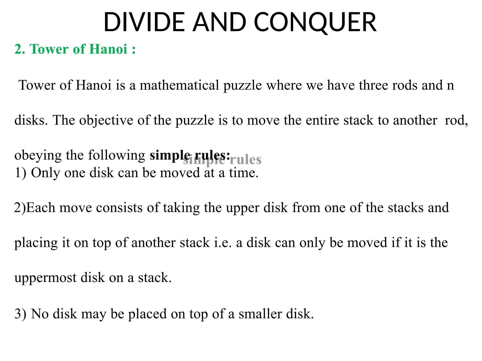
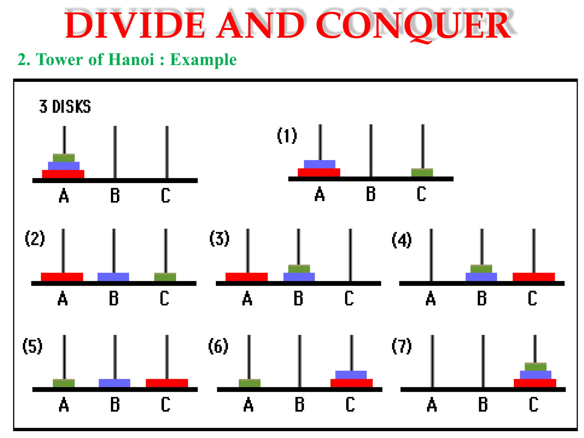
2. Tower of Hanoi :
Tower of Hanoi is a mathematical puzzle where we have three rods and n
disks. The objective of the puzzle is to move the entire stack to another rod,
obeying the following simple rules:
1) Only one disk can be moved at a time.
2)Each move consists of taking the upper disk from one of the stacks and
placing it on top of another stack i.e. a disk can only be moved if it is the
uppermost disk on a stack.
3) No disk may be placed on top of a smaller disk.

56. DIVIDE AND CONQUER
2. Tower of Hanoi : Example

57. GREEDY
STRATEGIES
Greedy algorithm :
An algorithm is designed to achieve an optimum solution for a given
problem. In the greedy algorithm approach, decisions are made from the
given solution domain. Being greedy, the closest solution that seems to
provide an optimum solution is chosen.
Example of greedy strategy :
1. Travelling Salesman Problem
2. Prim's Minimal Spanning Tree Algorithm
3. Kruskal's Minimal Spanning Tree Algorithm
4. Dijkstra's Minimal Spanning Tree Algorithm
5. Knapsack Problem
6. Job Scheduling Problem

58. GREEDY STRATEGIES
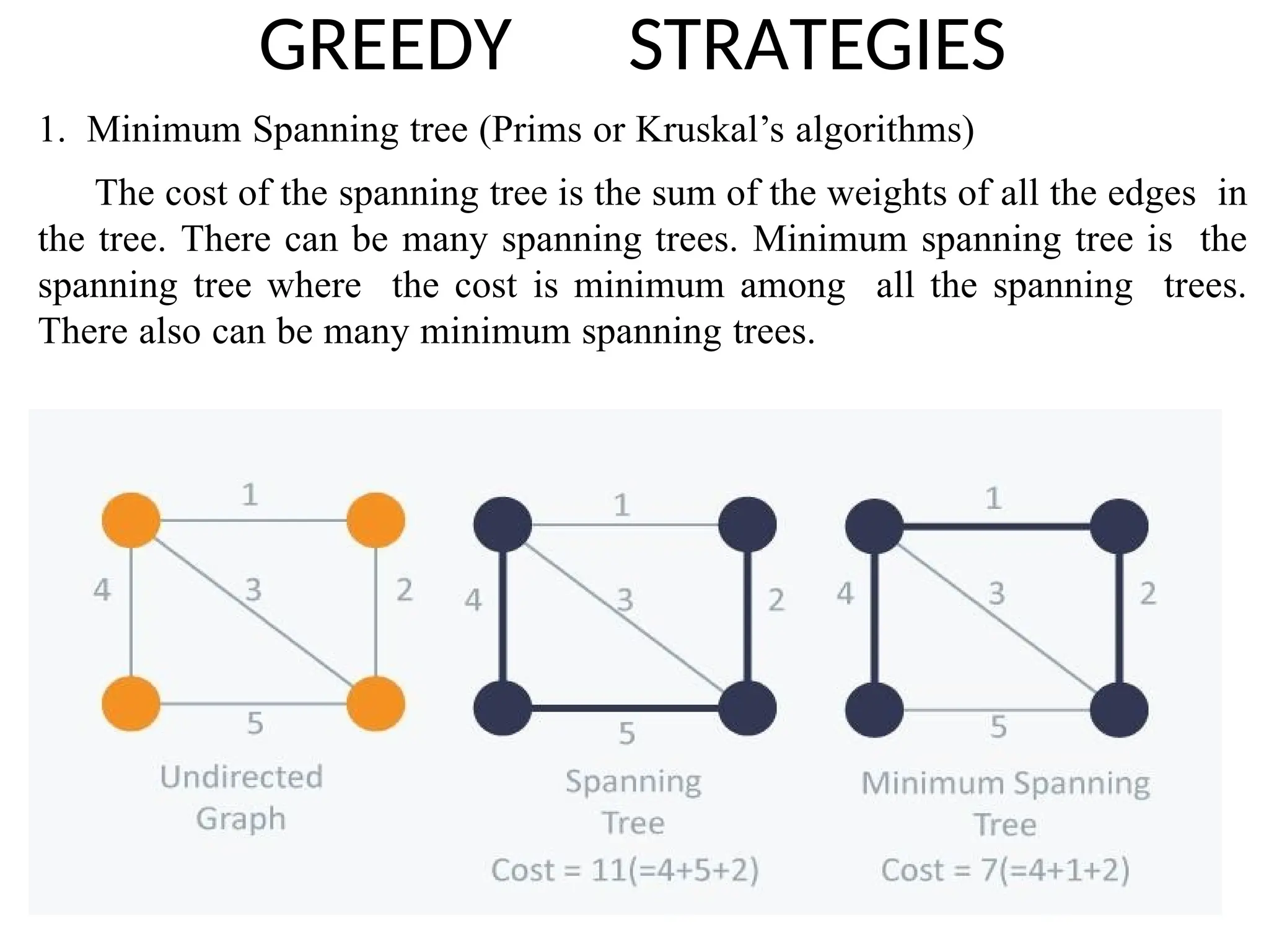
1. Minimum Spanning tree (Prims or Kruskal’s algorithms)
The cost of the spanning tree is the sum of the weights of all the edges in
the tree. There can be many spanning trees. Minimum spanning tree is the
spanning tree where the cost is minimum among all the spanning trees.
There also can be many minimum spanning trees.

59. GREEDY STRATEGIES
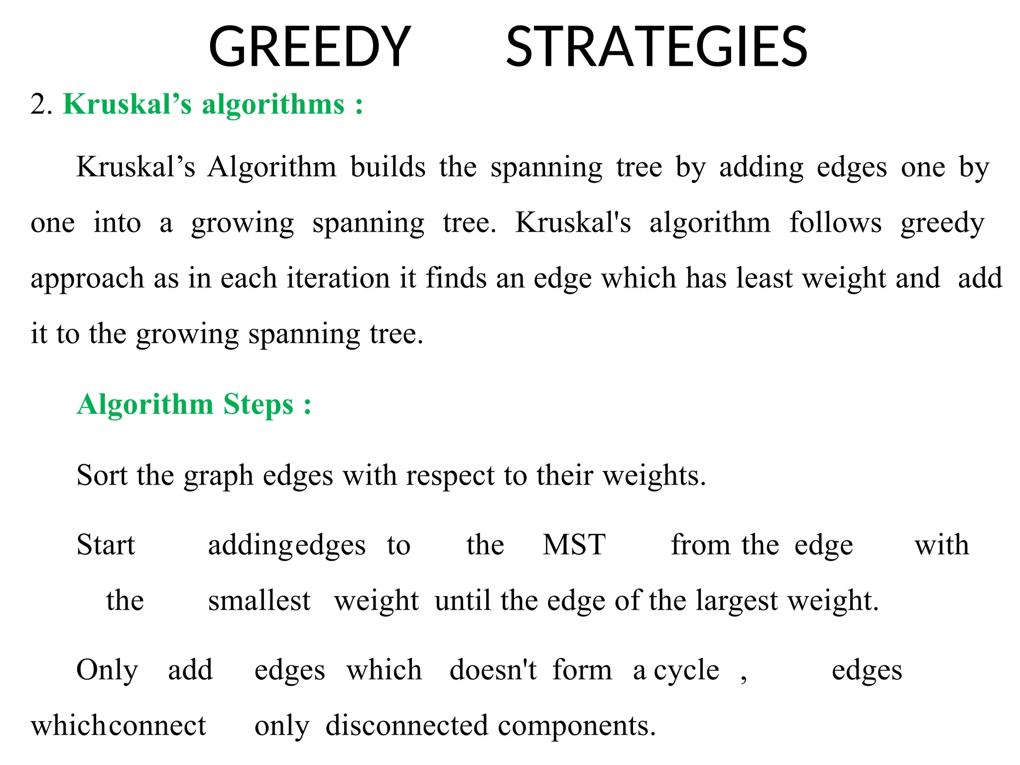
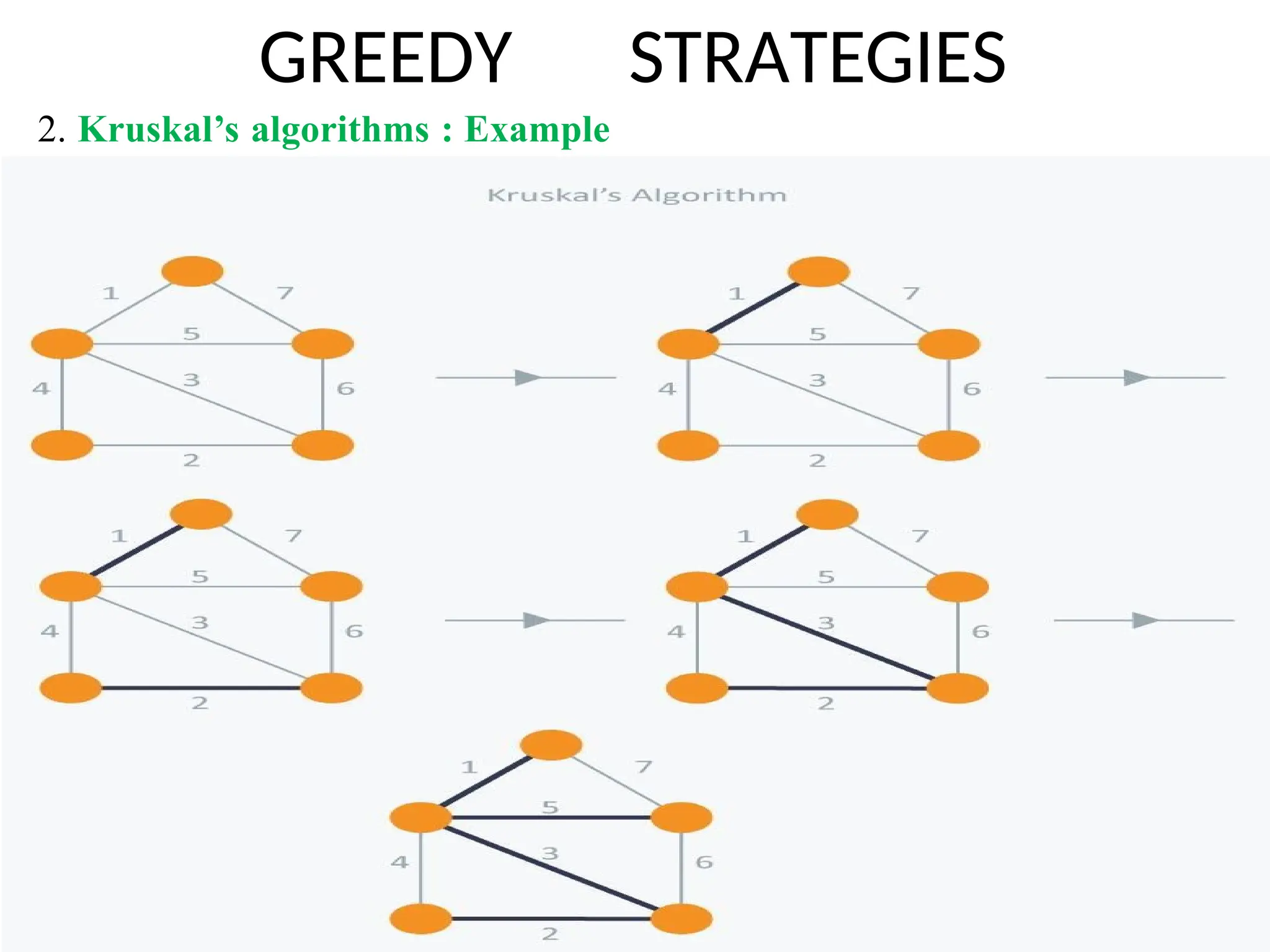
2. Kruskal’s algorithms :
Kruskal’s Algorithm builds the spanning tree by adding edges one by
one into a growing spanning tree. Kruskal's algorithm follows greedy
approach as in each iteration it finds an edge which has least weight and add
it to the growing spanning tree.
Algorithm Steps :
Sort the graph edges with respect to their weights.
Start addingedges to the MST from the edge with
the smallest weight until the edge of the largest weight.
Only add edges which doesn't form a cycle , edges
whichconnect only disconnected components.

60. GREEDY STRATEGIES
2. Kruskal’s algorithms : Example
.

61. GREEDY STRATEGIES
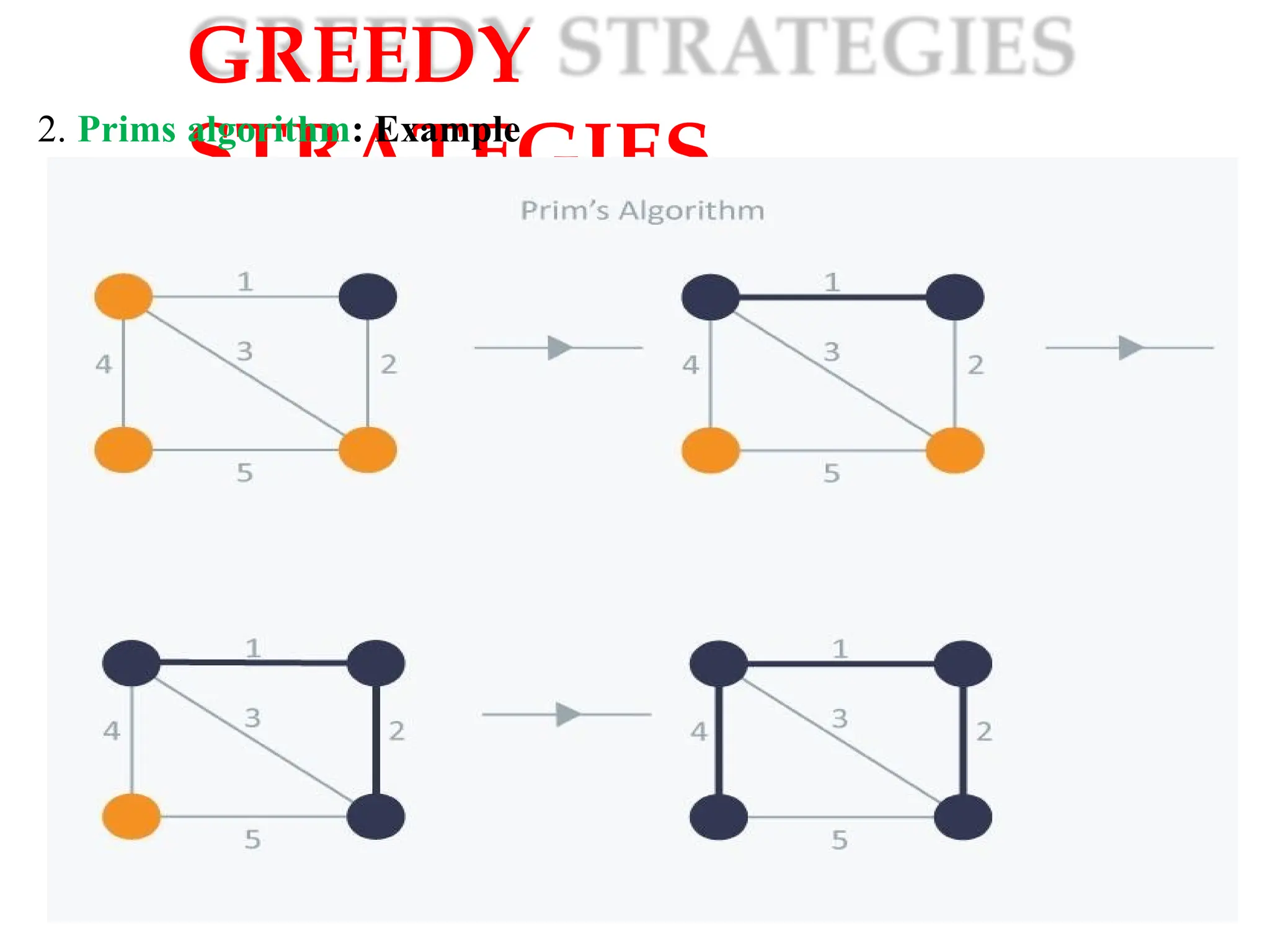
2. Prims algorithm: Prim’s Algorithm also use Greedy approach to find the
minimum spanning tree. In Prim’s Algorithm we grow the spanning tree
from a starting position. Unlike an edge in Kruskal's, we add
vertex to the growing spanning tree in Prim's.
Algorithm Steps:
1. Initialize the minimum spanning tree with a vertex chosen at random.
2.Find all the edges that connect the tree to new vertices, find the minimum
and add it to the tree.
3. Keep repeating step 2 until we get a minimum spanning tree.

62. GREEDY
STRATEGIES
2. Prims algorithm: Example

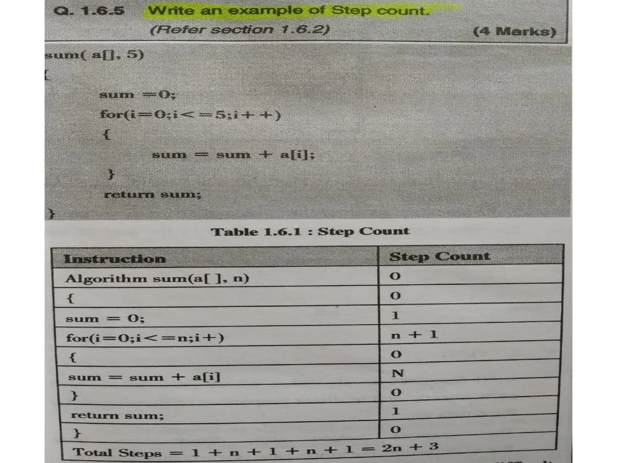
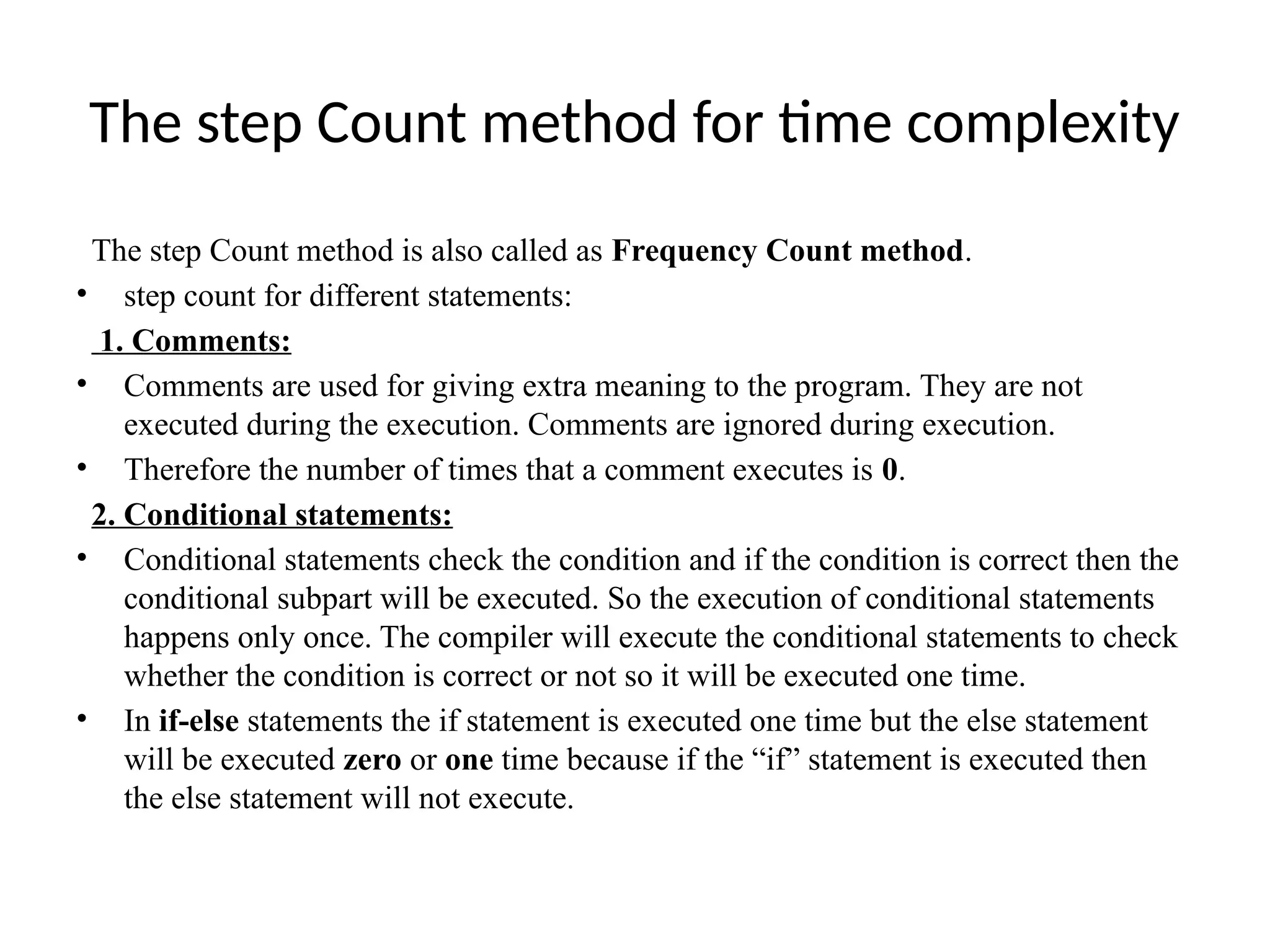
63. The step Count method for time complexity
The step Count method is also called as Frequency Count method.
• step count for different statements:
1. Comments:
• Comments are used for giving extra meaning to the program. They are not
executed during the execution. Comments are ignored during execution.
• Therefore the number of times that a comment executes is 0.
2. Conditional statements:
• Conditional statements check the condition and if the condition is correct then the
conditional subpart will be executed. So the execution of conditional statements
happens only once. The compiler will execute the conditional statements to check
whether the condition is correct or not so it will be executed one time.
• In if-else statements the if statement is executed one time but the else statement
will be executed zero or one time because if the “if” statement is executed then
the else statement will not execute.

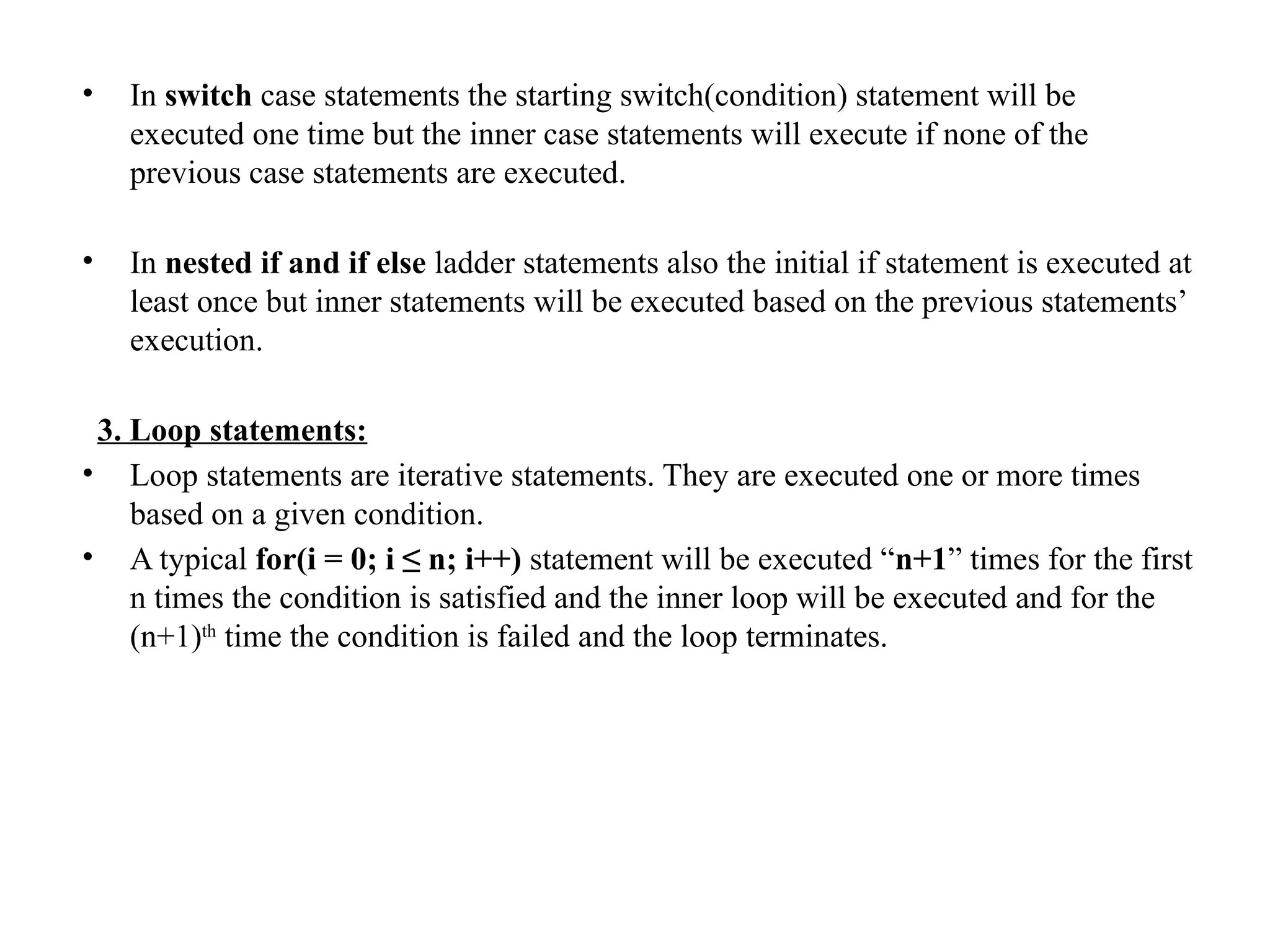
64. • In switch case statements the starting switch(condition) statement will be
executed one time but the inner case statements will execute if none of the
previous case statements are executed.
• In nested if and if else ladder statements also the initial if statement is executed at
least once but inner statements will be executed based on the previous statements’
execution.
3. Loop statements:
• Loop statements are iterative statements. They are executed one or more times
based on a given condition.
• A typical for(i = 0; i ≤ n; i++) statement will be executed “n+1” times for the first
n times the condition is satisfied and the inner loop will be executed and for the
(n+1)th
time the condition is failed and the loop terminates.

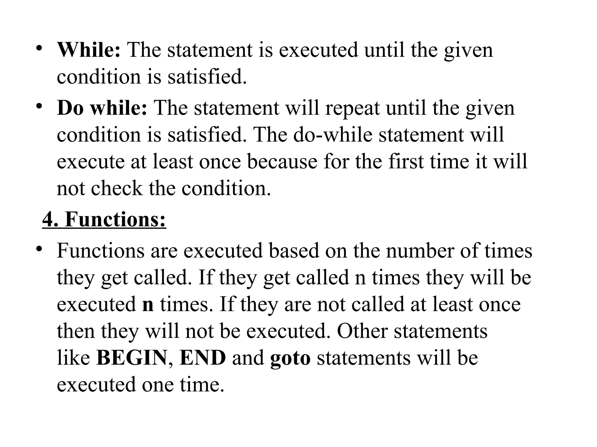
65. • While: The statement is executed until the given
condition is satisfied.
• Do while: The statement will repeat until the given
condition is satisfied. The do-while statement will
execute at least once because for the first time it will
not check the condition.
4. Functions:
• Functions are executed based on the number of times
they get called. If they get called n times they will be
executed n times. If they are not called at least once
then they will not be executed. Other statements
like BEGIN, END and goto statements will be
executed one time.

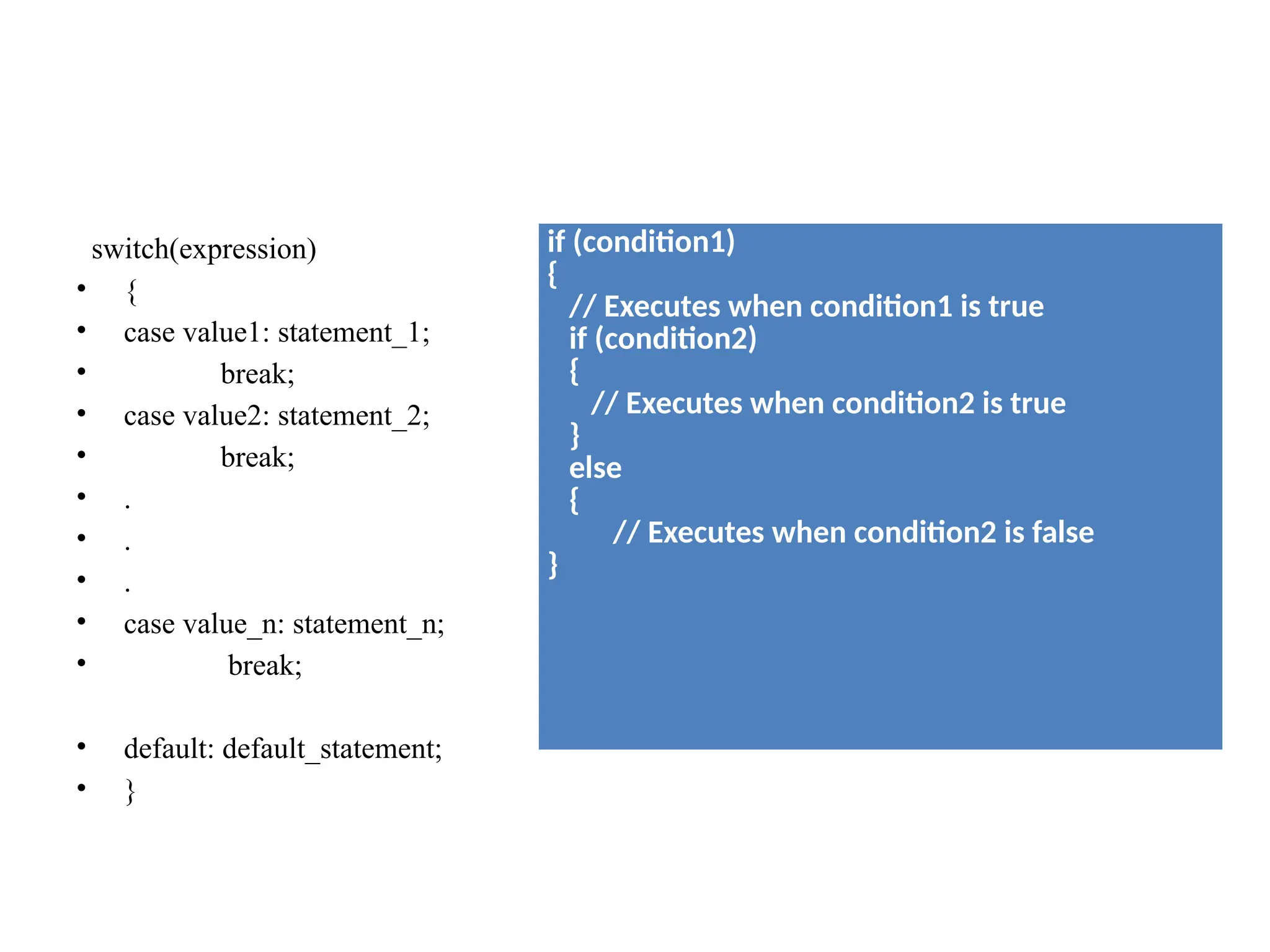
66. switch(expression)
• {
• case value1: statement_1;
• break;
• case value2: statement_2;
• break;
• .
• .
• .
• case value_n: statement_n;
• break;
• default: default_statement;
• }
if (condition1)
{
// Executes when condition1 is true
if (condition2)
{
// Executes when condition2 is true
}
else
{
// Executes when condition2 is false
}

67. Analysis of Linear Search algorithm
Let us consider a Linear Search Algorithm.
Linearsearch(arr, n, key)
{
i = 0;
for(i = 0; i < n; i++)
{
if(arr[i] == key)
{
printf(“Found”);
}
}

68. Where,
i = 0, is an initialization statement and takes O(1) times.
for(i = 0;i < n ; i++), is a loop and it takes O(n+1) times .
if(arr[i] == key), is a conditional statement and takes O(1)
times.
printf(“Found”), is a function and that takes O(0)/O(1) times.
Therefore Total Number of times it is executed is n + 4 times.
As we ignore lower exponents in time complexity total time
became O(n).
Time complexity: O(n).

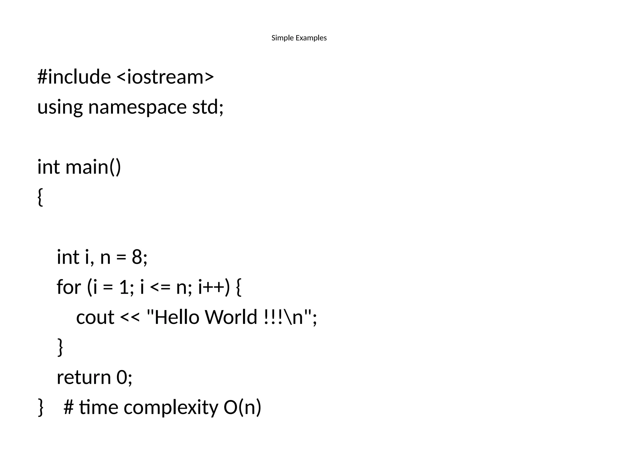
69. Simple Examples
#include <iostream>
using namespace std;
int main()
{
int i, n = 8;
for (i = 1; i <= n; i++) {
cout << "Hello World !!!n";
}
return 0;
} # time complexity O(n)

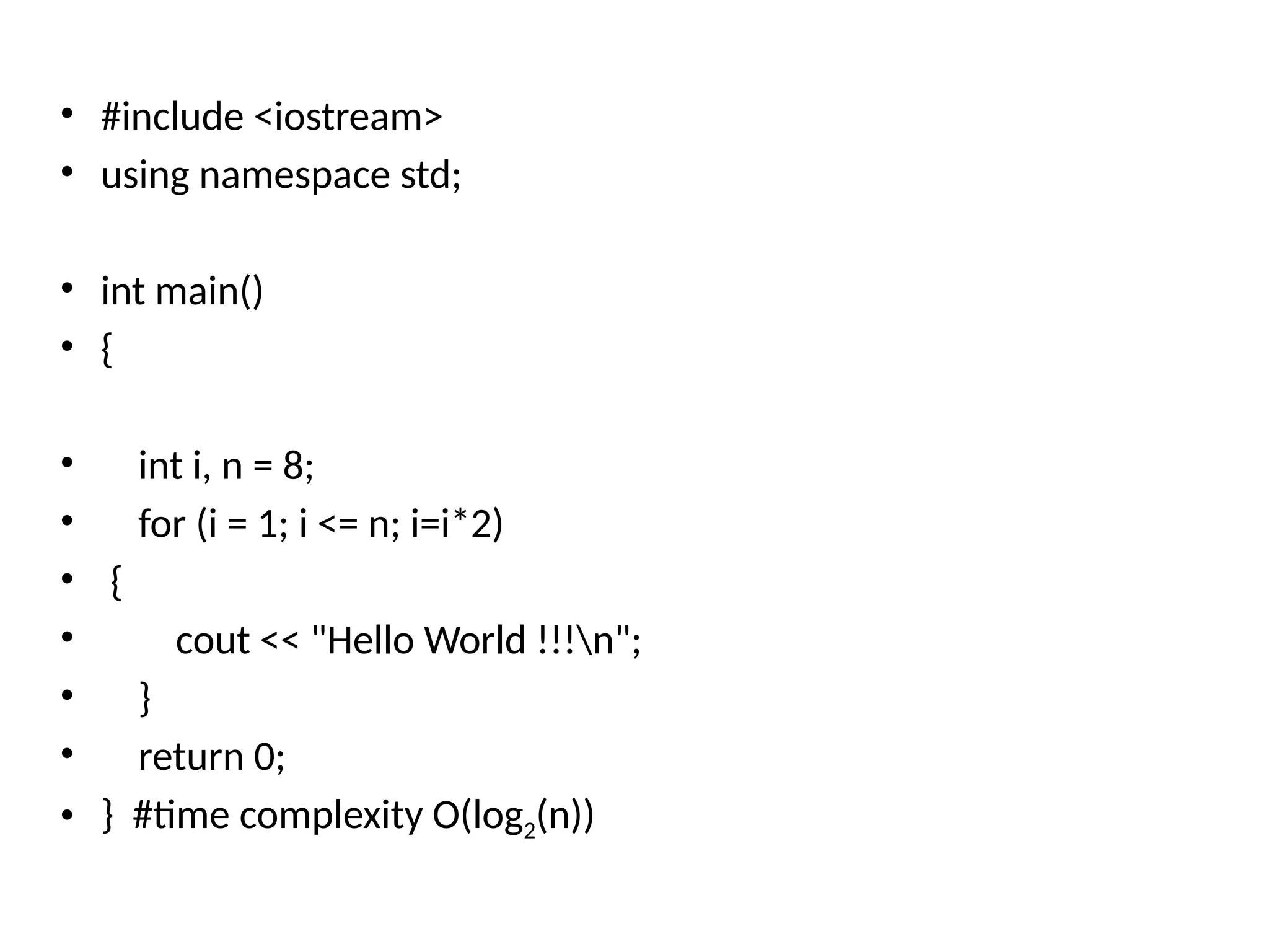
70. • #include <iostream>
• using namespace std;
• int main()
• {
• int i, n = 8;
• for (i = 1; i <= n; i=i*2)
• {
• cout << "Hello World !!!n";
• }
• return 0;
• } #time complexity O(log2(n))

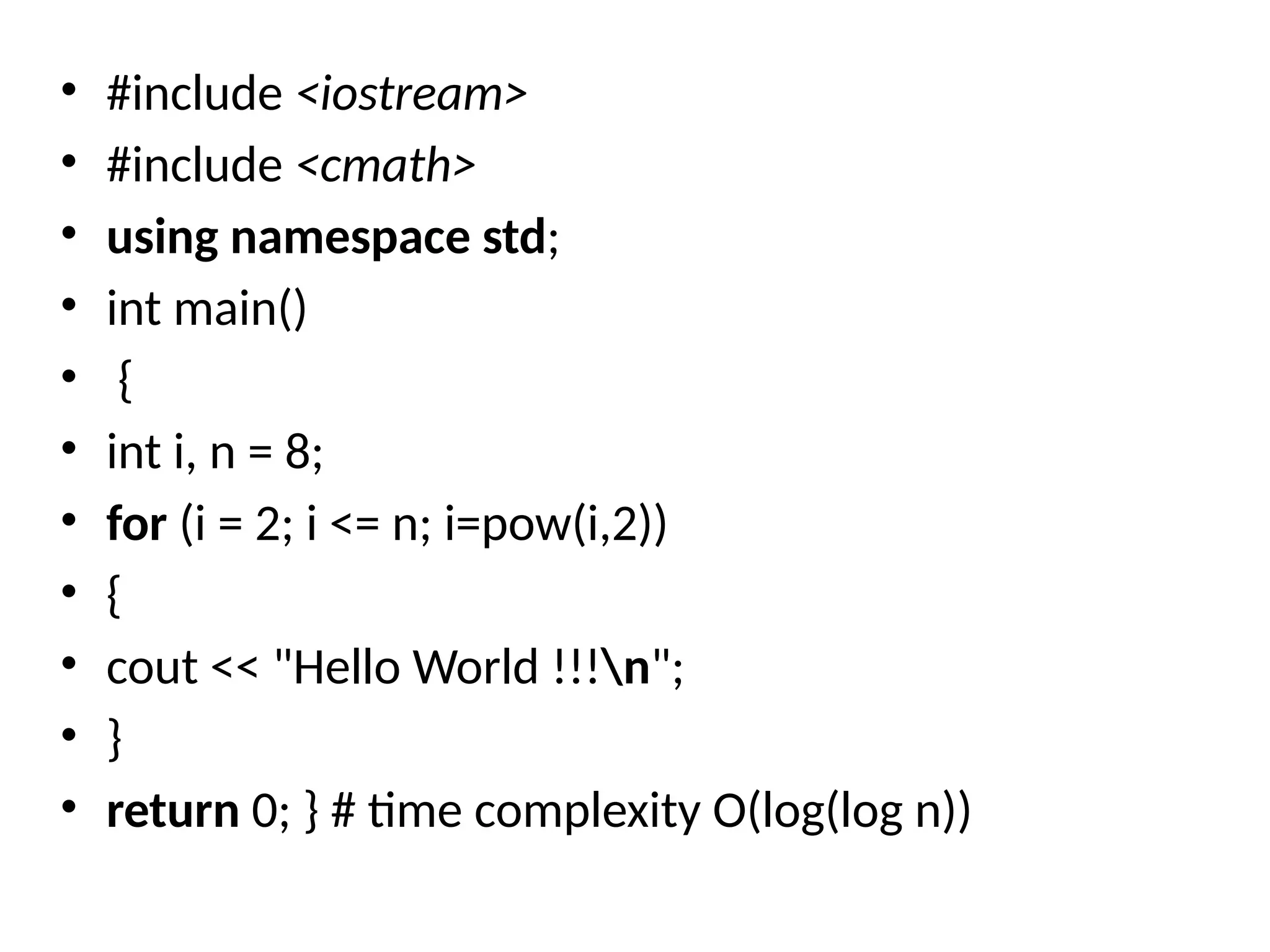
71. • #include <iostream>
• #include <cmath>
• using namespace std;
• int main()
• {
• int i, n = 8;
• for (i = 2; i <= n; i=pow(i,2))
• {
• cout << "Hello World !!!n";
• }
• return 0; } # time complexity O(log(log n))

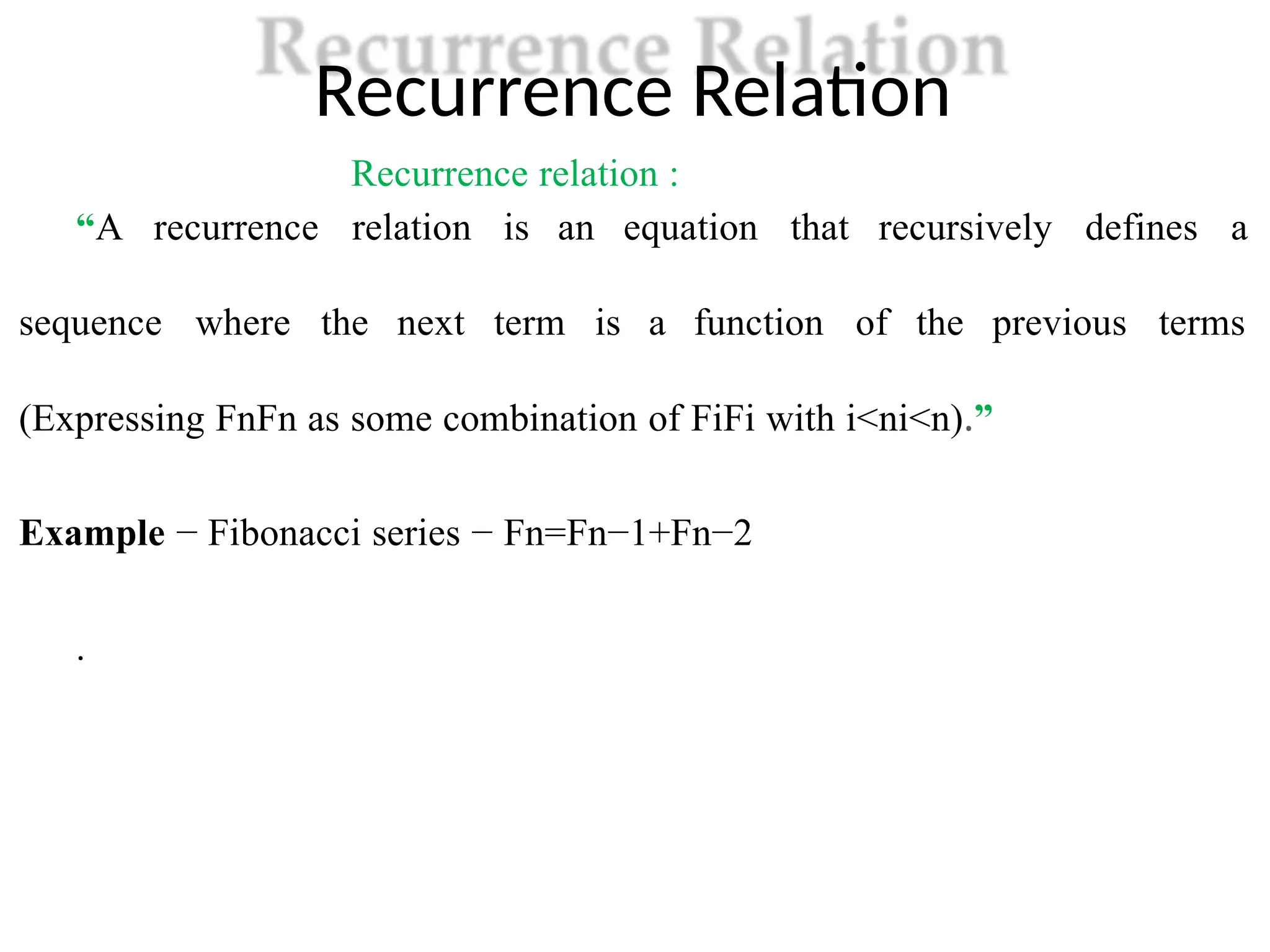
72. Recurrence Relation
Recurrence relation :
“A recurrence relation is an equation that recursively defines a
sequence where the next term is a function of the previous terms
(Expressing FnFn as some combination of FiFi with i<ni<n).”
Example − Fibonacci series − Fn=Fn−1+Fn−2
.

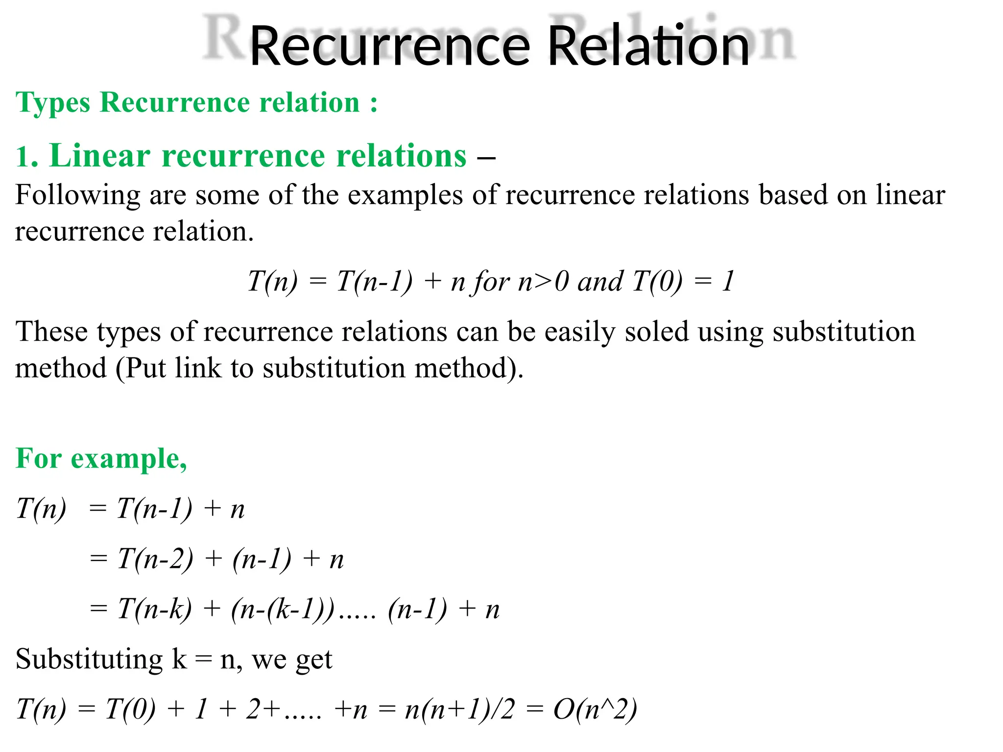
73. Recurrence Relation
Types Recurrence relation :
1. Linear recurrence relations –
Following are some of the examples of recurrence relations based on linear
recurrence relation.
T(n) = T(n-1) + n for n>0 and T(0) = 1
These types of recurrence relations can be easily soled using substitution
method (Put link to substitution method).
For example,
T(n) = T(n-1) + n
= T(n-2) + (n-1) + n
= T(n-k) + (n-(k-1))….. (n-1) + n
Substituting k = n, we get
T(n) = T(0) + 1 + 2+….. +n = n(n+1)/2 = O(n^2)

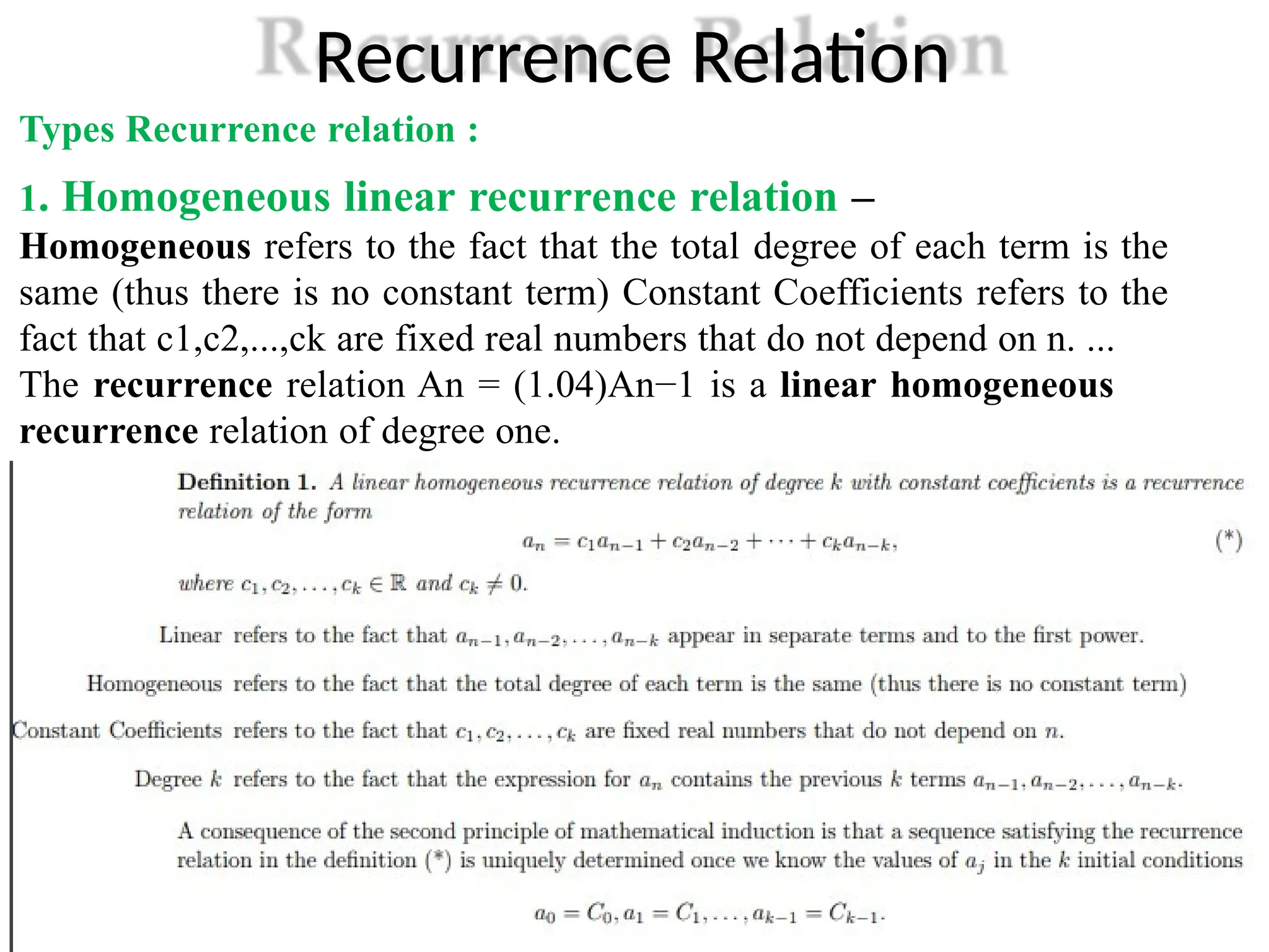
74. Recurrence Relation
Types Recurrence relation :
1. Homogeneous linear recurrence relation –
Homogeneous refers to the fact that the total degree of each term is the
same (thus there is no constant term) Constant Coefficients refers to the
fact that c1,c2,...,ck are fixed real numbers that do not depend on n. ...
The recurrence relation An = (1.04)An−1 is a linear homogeneous
recurrence relation of degree one.
.

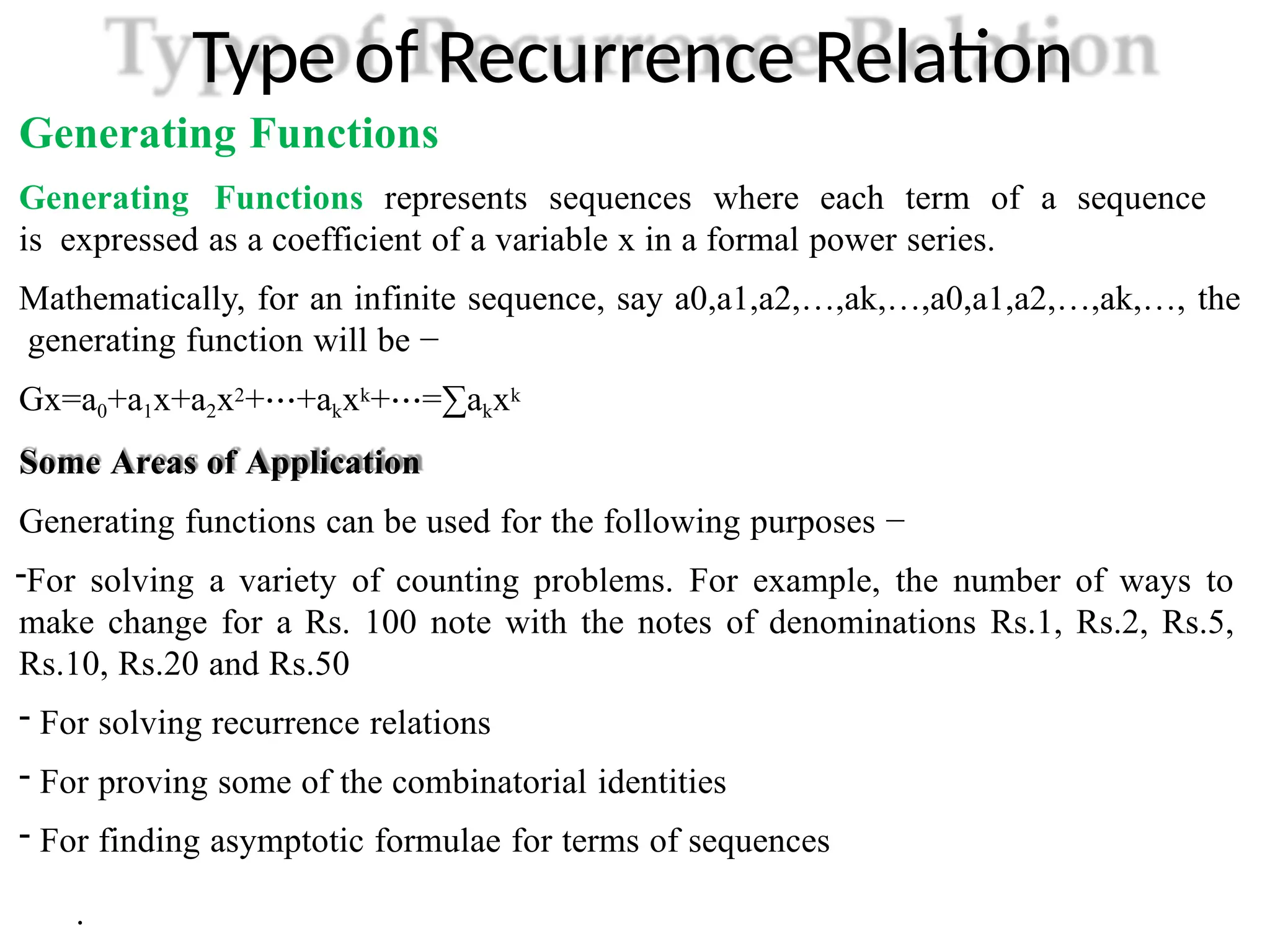
75. Type of Recurrence Relation
Generating Functions
Generating Functions represents sequences where each term of a sequence
is expressed as a coefficient of a variable x in a formal power series.
Mathematically, for an infinite sequence, say a0,a1,a2,…,ak,…,a0,a1,a2,…,ak,…, the
generating function will be −
Gx=a0+a1x+a2x2+⋯+akxk+⋯=∑akxk
Some Areas of Application
Generating functions can be used for the following purposes −
-For solving a variety of counting problems. For example, the number of ways to
make change for a Rs. 100 note with the notes of denominations Rs.1, Rs.2, Rs.5,
Rs.10, Rs.20 and Rs.50
- For solving recurrence relations
- For proving some of the combinatorial identities
- For finding asymptotic formulae for terms of sequences
.