Transactions On Computational Systems Biology Xiii 1st Edition Antti Hkkinen
Transactions On Computational Systems Biology Xiii 1st Edition Antti Hkkinen
Transactions On Computational Systems Biology Xiii 1st Edition Antti Hkkinen
Transactions On Computational Systems Biology Xiii 1st Edition Antti Hkkinen
Transactions On Computational Systems Biology Xiii 1st Edition Antti Hkkinen
1.
Transactions On ComputationalSystems Biology
Xiii 1st Edition Antti Hkkinen download
https://ebookbell.com/product/transactions-on-computational-
systems-biology-xiii-1st-edition-antti-hkkinen-2478234
Explore and download more ebooks at ebookbell.com
2.
Here are somerecommended products that we believe you will be
interested in. You can click the link to download.
Transactions On Computational Systems Biology Xiii 1st Edition Antti
Hkkinen
https://ebookbell.com/product/transactions-on-computational-systems-
biology-xiii-1st-edition-antti-hkkinen-4143750
Transactions On Computational Systems Biology Xii Special Issue On
Modeling Methodologies 1st Edition Rainer Breitling
https://ebookbell.com/product/transactions-on-computational-systems-
biology-xii-special-issue-on-modeling-methodologies-1st-edition-
rainer-breitling-4143748
Transactions On Computational Systems Biology Viii Priami
Corradoeditor
https://ebookbell.com/product/transactions-on-computational-systems-
biology-viii-priami-corradoeditor-20009668
Transactions On Computational Systems Biology X 1st Edition Agostino
Forestiero
https://ebookbell.com/product/transactions-on-computational-systems-
biology-x-1st-edition-agostino-forestiero-2040178
3.
Transactions On ComputationalSystems Biology Xi Muffy Calder
https://ebookbell.com/product/transactions-on-computational-systems-
biology-xi-muffy-calder-4143746
Transactions On Computational Systems Biology Xiv Special Issue On
Computational Models For Cell Processes 1st Edition Oana Andrei
https://ebookbell.com/product/transactions-on-computational-systems-
biology-xiv-special-issue-on-computational-models-for-cell-
processes-1st-edition-oana-andrei-4202966
Transactions On Computational Systems Biology Ii 1st Edition Guillaume
Blin
https://ebookbell.com/product/transactions-on-computational-systems-
biology-ii-1st-edition-guillaume-blin-4239040
Transactions On Computational Systems Biology Iv 1st Edition Robin
Milner Auth
https://ebookbell.com/product/transactions-on-computational-systems-
biology-iv-1st-edition-robin-milner-auth-4239368
Transactions On Computational Systems Biology V 1st Edition Zhong
Huang
https://ebookbell.com/product/transactions-on-computational-systems-
biology-v-1st-edition-zhong-huang-4239628
6.
Lecture Notes inBioinformatics 6575
Edited by S. Istrail, P. Pevzner, and M. Waterman
Editorial Board: A. Apostolico S. Brunak M. Gelfand
T. Lengauer S. Miyano G. Myers M.-F. Sagot D. Sankoff
R. Shamir T. Speed M. Vingron W. Wong
Subseries of Lecture Notes in Computer Science
8.
Corrado Priami Ralph-JohanBack
Ion Petre Erik de Vink (Eds.)
Transactions on
Computational
Systems Biology XIII
1 3
Preface
The many facetsof life are reflected by the multitude of dimensions of sys-
tems biology research at present. Current modeling and analysis approaches
to a systematic understanding of biological phenomena range from quantita-
tive to qualitative, from discrete to continuous, from deterministic to stochastic,
from concrete detailed biological case studies to abstract bio-inspired computing
paradigms. This special issue of the Transactions on Computational Systems Bi-
ology on Computational Models for Cell Processes also mirrors the rich variety
of the field.
The volume is based on the CompMod workshop that took place in Eind-
hoven, the Netherlands, on November 2, 2009. Previously held in Turku, Finland,
the workshop was organized for the second time, now as a satellite event of the
16th International Symposium on Formal Methods, part of FMweek, running
from November 2 to 6, 2009 in Eindhoven. The CompMod workshop aims to
foster a platform gathering researchers in formal methods and related fields in-
terested in the wealth of challenges and opportunities in systems biology. A
specific interest is expressed for papers discussing biological processes requiring
special tools and techniques not investigated so far in the context of formal meth-
ods, as well as extensions of formal methods formalisms introduced to improve
their applicability to biology. For this special issue there has been an additional
open call for paper submissions, with a separate peer-reviewing process.
The papers included illustrate the broad span of aspects of modeling and
analysis of biological systems: evolution of a cell population with selection based
on toxin resistance; a quantitative and tool-supported interpretation of flow ab-
straction in the Systems Biology Graphical Notation; an analytic approach to
dynamic simulation of deformable biological structures; a new stochastic simula-
tion algorithm reconsidering the delay-as-duration principle; a process algebraic
case study on ammonium transport in plant-fungus symbiosis; iterative variable
elimination for steady state equations using algebraic modules in the analysis
of metabolic networks. From different points of view and following various ap-
proaches the papers cover a wide range of topics in Systems Biology, addressing
the dynamics we begin to unravel and computational principles that we start to
identify.
This issue also includes two regular papers by Wallace and Wallace on the
heritability of complex diseases and by Paulevé et al. on the dynamics of gene
regulatory networks.
December 2010 Ralph-Johan Back
Ion Petre
Corrado Priami
Erik de Vink
12.
LNCS Transactions on
ComputationalSystems Biology –
Editorial Board
Corrado Priami, Editor-in-chief University of Trento, Italy
Charles Auffray Genexpress, CNRS
and Pierre & Marie Curie University, France
Matthew Bellgard Murdoch University, Australia
Soren Brunak Technical University of Denmark, Denmark
Luca Cardelli Microsoft Research Cambridge, UK
Zhu Chen Shanghai Institute of Hematology, China
Vincent Danos CNRS, University of Paris VII, France
Eytan Domany Center for Systems Biology, Weizmann Institute, Israel
Walter Fontana Santa Fe Institute, USA
Takashi Gojobori National Institute of Genetics, Japan
Martijn A. Huynen Center for Molecular and Biomolecular Informatics,
The Netherlands
Marta Kwiatkowska University of Birmingham, UK
Doron Lancet Crown Human Genome Center, Israel
Pedro Mendes Virginia Bioinformatics Institute, USA
Bud Mishra Courant Institute and Cold Spring Harbor Lab, USA
Satoru Miayano University of Tokyo, Japan
Denis Noble University of Oxford, UK
Yi Pan Georgia State University, USA
Alberto Policriti University of Udine, Italy
Magali Roux-Rouquie CNRS, Pasteur Institute, France
Vincent Schachter Genoscope, France
Adelinde Uhrmacher University of Rostock, Germany
Alfonso Valencia Centro Nacional de Biotecnologa, Spain
Evolutionary Dynamics ofa Population of Cells
with a Toxin Suppressor Gene
Antti Häkkinen1
, Fred G. Biddle2
, Olli-Pekka Smolander1
,
Olli Yli-Harja1
, and Andre S. Ribeiro1,3
1
Computational Systems Biology Research Group,
Tampere University of Technology, Finland
2
Department of Medical Genetics, Institute of Maternal and Child Health,
Faculty of Medicine, University of Calgary, Canada
3
Center for Computational Physics, University of Coimbra,
P-3004-516 Coimbra, Portugal
Abstract. Environmental changes are known to trigger evolutionary
changes, e.g. by favoring higher mutation rates. We study the evolution-
ary dynamics of a delayed stochastic genetic circuit using a simulator de-
veloped for this aim. We model a cell population subject to selection and
environmental changes. Each cell contains a self-repressing gene whose
protein degrades a toxin. Allowing mutations, we study the adaptability
of this circuit and how the genotypic and phenotypic diversities of the
population evolve. Neutral mutations and equally beneficial evolution-
ary pathways are found to generate complex phenotypic distributions.
We find optimal mutation rates dependent on the amount of toxin and
show that shifting environmental conditions trigger transient increases
in diversity. The results support the hypothesis that evolvability is a
selectable trait.
1 Introduction
Organisms adapt to a wide range of unpredictable environmental changes. Geno-
typic and phenotypic diversity, which play a major role in the organisms’ poten-
tial to adapt to changes, are likely to be heritable and to be partially responsible
for organisms’ robustness [1]. Especially in prokaryotes, noise in gene expression
is a key source of phenotypic diversity [2,3]. Another source is the interaction
between organisms and the environment [4].
In unstable environments, organisms are likely to need higher mutation rates,
unlike in more stable conditions, as high mutation rates tend to cause the ac-
cumulation of deleterious mutations [5]. Selection can only act when there is
variability within a population [6]. Since variability depends on the mutation
rate, the ability to control this rate is a selectable trait. In support of this hy-
pothesis, bacterial mutation rates were found to increase in the initial stages of
colonization of a mouse gut [7], decreasing afterwards.
The ability to generate heritable phenotypic variation is a selectable trait [1].
One such case has been characterized in Bacillus subtilis, which has probabilis-
tic and transient cellular differentiation, dependent on the environment [8]. The
C. Priami et al. (Eds.): Trans. on Comput. Syst. Biol. XIII, LNBI 6575, pp. 1–12, 2011.
c
Springer-Verlag Berlin Heidelberg 2011
17.
2 A. Häkkinenet al.
probability of being in either state is stationary within a given external condi-
tion, and is determined by the noise in ComK expression level [8]. Reduction of
the noise decreases the number of competent cells, suggesting that noise-driven
genetic mechanisms can evolve [9].
Here, we study the evolutionary dynamics of a self-repressing gene responsible
for coping with a toxin, and whose dynamics is driven by a delayed stochastic
simulation algorithm, at the single molecule level. Each model cell has a gene
responsible for resistance to tetracycline that has been characterized in biolu-
minescent Escherichia coli K-12 [10]. Tetracycline resistance is regulated by the
tetA promoter and the TetR protein, which acts as a self-repressor. In the ab-
sence of tetracycline, the TetR protein binds to the promoter and represses own
expression that was induced when tetracycline was added [10]. The model envi-
ronment consists of the amount of exposure of each cell to the toxin tetracycline.
We address the following questions: Do genotypic and phenotypic diversity
depend on environmental conditions? How does the rate of change of the envi-
ronment affect these diversities? Are there optimal mutation rates for a given
environment?
2 Methods
We simulate, at the single cell level, cell populations that are subject to selec-
tion at the end of each generation. The dynamics of each cell is driven by the
delayed Stochastic Simulation Algorithm [11], based on the original SSA [12],
and implemented in SGNSim [13]. The model of gene expression [14] accounts
for stochastic fluctuations and, by using multiple-time delayed reactions, it ac-
counts for the fact that transcription and translation are multiple-step processes
and take non-negligible time to be completed once they are initiated. The model
was validated by matching measurements of the time series of gene expression
at the single molecule level [15,16]. Time delayed reactions are represented as:
A + C → A(τ1 ) + B(τ2 ) + D. When the reaction occurs, C is instantaneously
consumed, and D is instantaneously produced. Substance A is not consumed
but it is placed on a waitlist until it is released after τ1 s, while a new substance
B is produced τ2 s after the reaction occurs [11,13].
To model mutations and cell selection, we developed and implemented a wrap-
per program for SGNSim, named “CellSelector”. CellSelector allows running
multiple independent simulations of single gene models in parallel for a specified
time length, which corresponds to the cells lifetime. In our simulations, for each
set of conditions, we run 100 independent threads. The simulation of the dy-
namics of each cell is seeded with a unique seed to initialize the random number
generator, responsible for the generation of the stochasticity of the simulation
according to the SSA, thus guaranteing that the cells in each generation have
unique trajectories in the state space. The simulator program is available upon
request.
After the fixed lifetime of the cells of a generation is past, the final state of
the each cell is observed. Selection then occurs, based on these states. Namely,
18.
Evolutionary Dynamics ofa Population of Cells 3
the cells are sorted by a fitness measure fit, and those belonging to the least
fit q-quantile are eliminated, while the others are used to produce two or more
duplicates for the subsequent cell generation. In our simulations we always elim-
inate 50% of the cells at the end of each generation, and make two duplicate
cells out of each of the remaining cells that will constitute the cell population of
the next generation.
The initial state of the daughter cells is set to be identical to the final state
of their mother cell (with a new random seed being generated for each daughter
cell). This implies that any mutations accumulated by the mother cell are present
in the daughter cells. Only the fitness measure is set to zero at the beginning of
each cell lifetime.
When toxin is present, it binds to protein p (even when the protein is bound
to the promoter), which therefore can no longer repress the gene, allowing tran-
scription to take place. Being a stochastic system, the higher the number of
toxins in the cell, the more likely it is that the promoter is free to transcribe.
At any given moment, we define “environmental conditions” as the number of
toxins that the cell is subject to.
The environmental conditions determine both how much time cells are subject
to the toxin and the amount of toxin. Toxin (“X”) is introduced in the cells
via reaction (1) at rate cpois (the value of this rate defines the environmental
condition at any given moment) and degrades via reaction (2) at rate dpois .
These reactions are only active when the cell is subject to toxin, and they
impose approximately constant amount of toxin over time during these periods.
Tuning cpois allows controlling such amount:
cpois
−→ X (1)
X
dpois
−→ ∅ (2)
A cell’s fitness is measured throughout its life. The toxin is assumed to be harm-
ful. Excess of protein is also assumed harmful, since in the case of the gene
studied here it leads to cell death due to loss of membrane potential [17]. Thus,
we assume that the goal of each cell and the selection process is to simultane-
ously decrease the amounts of toxin and protein. Finally, in order to inactive a
toxin X , a protein p needs to bind to it, forming the complex Xp. The number
of Xp complexes is a good indicator of the fitness of the cell.
Combining these conditions, fitness is stochastically measured by reaction
(3) (the symbol ∗
indicates that the reactant is not consumed in the reaction,
although it affects the propensity of the reaction [13]):
∗
X +∗
p +∗
Xp
cfit
−→ fit (3)
The propensity (Prop(4)) [12] of reaction (3) is calculated at each step of the
stochastic simulation by equation (4):
Prop(4) = cfitr × ([X] + 1)−1
× ([p] + 1)−1
× ([Xp] + 1) (4)
19.
4 A. Häkkinenet al.
Note, from reaction (3) and the formula used to compute its propensity (4), that
the more toxins X and proteins p exist in the cell, the less fitness units, fit, will
be produced. For that to be possible in the simulation, following the protocols of
SGNSim [13], we introduced in the left hand side of the reaction X and p, so as
to allow the propensity of the reaction to be inversely dependent on the amounts
of these two substances, since the speed of production of fit is determined by
the propensity (defined in (4)) [12].
Reaction (3) doesn’t affect the cells’ dynamics since no substance is consumed
and the product is not a substrate to any reaction. Its propensity [12] determines
how many fitness units are produced and is computed according to equation (4),
in agreement with the fitness conditions proposed. All cells have zero fitness
units in the beginning of their life.
To the best of our knowledge, this method of computing the fitness of a genetic
circuit at runtime by introducing a stochastic reaction in the system has not been
previously used. It is therefore important to note that the dynamics of the other
reactions in the system are not affected in any way, and that the value of fitness
has a stochastic component. According to the SSA, the number of times and the
moments when a reaction occurs is solely determined by its propensity at each
moment [12]. In our model, the dynamics of all other reactions (i.e., the number
and the moment of occurrence of the reactions) are not affected by the reaction
producing fitness units because it does not consume or produce any substances
associated to the other reactions, thereby not affecting their propensities at any
moment.
Further note that this is also true for reactions 13 and 14, since, as seen
later, they do not consume any substances affecting the propensities of the other
reactions in the system. In practical terms, our method is equivalent to, e.g.,
calculating fitness at runtime by having two parallel simulations ongoing simul-
taneously (one for the system, another for fitness calculation) with the latter
being informed of the state of the first at each step.
Additionally, it is noted that while the expression of the propensity of reaction
3 differs from common expressions of propensity of regular chemical reactions
(i.e. linear dependence on each substrate), this does not affect the dynamics or
functioning of the SSA or the simulator. SGNSim [13] uses the formula to obtain
a real value of propensity at each moment which, as in the other reactions,
determines the reaction’s stochastic rate of occurrence.
Gene expression is modeled by multiple time-delayed reactions, one for tran-
scription (5) by RNA polymerase (RNAp), with a stochastic rate constant kt,
and one for translation (6) by ribosomes (rib), with a stochastic rate constant
ktr, according to the model proposed in [14]. As mentioned, in these reactions,
the delays are represented explicitly. E.g. in reaction 5, the notation “RBS(2)”
denotes that the ribosome binding site is only produced and introduced in the
system 2s after the reaction occurs.
Decay reactions degrade p, (7 and 10) and RNA’s (represented by their ribo-
some binding site, RBS [16]) via reaction (8). Reactions (9) model the binding
and unbinding of the self-repressor protein to the gene promoter region (Pro).
20.
Evolutionary Dynamics ofa Population of Cells 5
The binding of X to p when free or when bound to the promoter [10] is modeled
by reactions (11) and (12).
Pro + RNAp
kt
−→ Pro(2) + RNAp(40) + RBS(2) (5)
RBS + rib
ktr
−→ RBS(2) + rib(20) + p(50) (6)
p
dp
−→ ∅ (7)
RBS
dRBS
−→ ∅ (8)
Pro + p
kunrep
krep
Pro.p (9)
Pro.p
dp
−→ Pro (10)
X + p
kpdes
−→ X.p (11)
X + Pro.p
kpdes
−→ X.p + Pro (12)
We assume that the gene is subject to mutations, and that these affect the
rate of transcription as well as the strength of repression, since these rates are
those that most directly affect the rate of production of the protein. Thus, the
rates subject to changes due to mutations in the gene sequence (initiation and
elongation regions) are kt , krep, and kunrep. Affinity between promoter and pro-
tein determines krep and kunrep, while transcription initiation (kt ) is sequence
dependent [18].
We use virtual substances [13] to implement at runtime the effects of muta-
tions in a cell’s dynamics. The propensity of reactions (5) and (9) is computed
as follows. Let K be the original rate constant, nup be a virtual substance that
increases the reaction propensity if its quantity increases, and ndown a virtual
substance that decreases the propensity if its quantity increases. To do this, the
propensity of the reaction, P, is computed by (13):
P = K × (nup + 1) ×
1
1 + ndown
(13)
The propensity can be varied at runtime by reactions (14) and (15). A pair of
reactions (14) and (15) is added for each rate constant subject to changes due
to mutations:
∅
kmut
−→ M × nup (14)
∅
kmut
−→ M × ndown (15)
21.
6 A. Häkkinenet al.
In reactions (14) to (15), tuning kmut allows varying the rate of occurrence of
mutations and by tuning M (number of molecules created in one reaction) one
can set the extent of the variation in the propensity caused by one mutation.
When any of the two reactions, (14) and (15) occur, nup or ndown vary, thus
changing the propensity of the reaction they affect (either transcription, repres-
sion or unrepression). If the change improves the cell fitness, this cell is likely to
be selected for duplication at the end of its lifetime.
It is noted that the rates subject to mutation, i.e. kt , krep, and kunrep, allow
varying both the mean expression as well as the noise strength of the protein
level. Also, due to the existence of the delay on the promoter release, identical
ratios between krep and kunrep will produce the same mean expression level, but
the RNA and the protein levels will have different noise strengths [19].
3 Results
Reactions (1-12), (14) and (15) are implemented in each cell. The unit of time
delays is second (s) and the unit of rate constants is s−1
. Since we model a
gene from E. coli [10] the parameters values are set accordingly, e.g, transla-
tion initiation (ktr = 0.0005 ), RNA decay (dRBS = 0.005 ), and protein decay
(dp = 0.0004 ) [16]. The same applies to the time delays in transcription (5) and
translation (6). The values of the delays are set according to known kinetic pa-
rameters of transcription and translation in E. coli (for a detailed justification
and derivation of the values of these delays please refer to [16]).
Cell division (and selection) occurs at each 1800 s, which is the average divi-
sion time of E. coli. Additionally, we set kpdes to 0.01 which is within realistic
parameter values [20], and cfit to 1.
To impose an average toxin concentration in the cell of, e.g., 10 molecules
X , we set cpois = 0.1 and dpois = 0.01. In a following simulation, cpois will be
varied to subject the cells to different environments at runtime.
The rates that are varying due to mutations are initially set to: kt = 0.0025 ,
krep = 10−4
, and kunrep = 0.1 . Real mutation rates in E. coli are ∼ 10−7
per
cell division, but vary significantly depending on the conditions to which cells
are subject [21]. We vary this rate (kmut ) to study its effects. Unless stated
otherwise, we model 100 cells per generation for 100 generations (100G).
We first tested the effects of varying M , with kmut = 10−4
. Cells are subject
to toxin for periods of 10G with cpois = 0.1 and dpois = 0.001 , interrupted by
periods of 10G not subject to toxin. For M ≤ 2, mutations effects are below the
noise level. Increases in the population’s fitness are only due to selection. For
2 M 10000 the average fitness increases for several generations and reach
a maximum value, equal for all values of M . It takes from 10G to 50G to reach
the maximum fitness.
Next we varied kmut from 10−7
to 1. We set M = 10, so that mutations
cause phenotypic changes significantly above the noise level. For kmut 10−6
and kmut 0.1, fitness only improves due to selection. In the first case, the
number of mutations that can occur within 100G is not sufficient to allow the
22.
Evolutionary Dynamics ofa Population of Cells 7
cells to adapt to the change and, in the second case, due to a too high mutation
rate, the selection that occurs at each generation is not sufficient to prevent the
accumulation of harmful mutations.
Setting kmut to 10−4
and M to 10, we now analyze the phenotypic diver-
sity in a simple environment, namely, where no toxin is present in the first
100G and where, from G100 to G200, cells are subject to toxin (cpois = 0.1 and
dpois = 10−3
) and, finally, no toxin is present thereafter.
To quantify the diversity of the values of the rate constants subject to changes
due to mutations over the population, we compute the ratio between standard
deviation and mean value of these rates, i.e. the coefficient of variation, CV , in
each generation.
In Fig. 1 we plotted the CV of kt, krep and kunrep for 300G. All CV ’s were
comparatively high, i.e. the population had higher phenotypic and genotypic
diversities, after environmental changes and in the initial transient, from G1
to ∼G30, where cells are adapting to an environment without toxin (evolving
towards diminishing the number of proteins by decreasing kt and/or increasing
krep). The other moments are from G100 to G140 and from G200 to G230, the
adaptation periods to the environmental changes (toxin introduced at G100 and
removed at G200). Thus, changes in the environment trigger transient increases
in genotypic and phenotypic diversities in the populations of model cells.
From these results we conclude that, even assuming fixed mutation rates for
simplicity, environmental changes are likely to enhance the degree of variability
of a population. When the environmental conditions change, cells that were
optimally adapted are no longer as fit as before. Thus, recently mutated cells
have greater chances to be fitter in variable environments (in comparison to non
mutated ones) than in stable ones.
In the periods that the cells are fittest (from G30 to G100, from G140 to
G200, and after G230), the population maintains a considerable diversity. This
is due both to the continuous appearance of mutated cells (usually removed in
subsequent generations) and neutral mutations, e.g., causing equal increases in
krep and kunrep, which does not change the average time the gene is repressed.
Neutral mutations are one of the causes for the emergence of complex pheno-
typic distributions (e.g., bimodal) and one example is shown in Fig. 2. In this case
some cells have higher krep than the rest of the population but also higher kunrep
(not shown). Another way for genotypic and consequent phenotypic bifurcations
to appear is when distinct evolutionary pathways have identical fitness, e.g., in-
stead of increasing krep, decreasing the transcription rate kt also diminishes the
number of p’s in the cell).
Finally, we subject populations of initially identical cells to various environ-
ments and measure the average fitness over 100 generations. Toxin is introduced
at random moments for random time durations. The transition rate between
presence and absence of toxin is set to 1/(10 × T) (where T is the cells life-
time). The environments differ in the amount of toxin present. We set cpois to
0.001, 0.1 and 1, while dpois is kept at 0.01. The results are shown in Fig. 3.
23.
8 A. Häkkinenet al.
Fig. 1. Coefficient of variation (CV ) of rates subject to mutation in 1 simulation of
300 cell generations. Toxin absent from G1 to G100 and from G200 to G300. Vertical
dashed lines represent the moments when the environmental conditions changed.
Fig. 2. Population genotypic distribution at G105 of the evolved values of the multi-
plicative factor of krep
There are optimal mutation rates (Fig. 3) whose values depend on the envi-
ronmental conditions, i.e., amounts of toxin. Because the model cells are initially
not well adapted to the presence of virtually no toxin, the higher the amount of
toxin introduced, the higher must be the mutation rate. That is, a determining
24.
Evolutionary Dynamics ofa Population of Cells 9
Fig. 3. Average fitness in 100 G for various toxin dosages and mutation rates
factor of the value of optimal mutation rates is the necessary genotypic and phe-
notypic change to reach maximum fitness. Initially, less well-adapted cells require
higher mutation rates to rapidly create diversity from which fitter cells can be
selected from. This suggests that it is advantageous for cells to tune or evolve
mutation rates depending on the environmental conditions and shifting of these
conditions.
Two factors contribute to the existence of optimal mutation rates of this gene:
if mutation rates are too low, beneficial mutations do not occur fast enough to
improve the population’s fitness in reasonable time and, if mutation rates are
too high, selection is not sufficiently fast to prevent the accumulation of harmful
mutations.
4 Conclusions and Discussion
We implemented in model cells a stochastic model with delays of a self-repressing
gene responsible for Tetracycline resistance [10] in E. coli. We simulated pop-
ulations of cells over several generations, subjecting each cell to a stochastic
environment and providing them the ability to mutate the dynamical properties
of this genetic circuit. At the end of each generation, we selected the fittest cells.
We investigated the role and evolvability of both mean expression as well as
noise strength of this gene, as key variables in the ability of the cell to cope
with changing environmental conditions. We further studied the consequences
of subjecting the cells to fluctuating environmental conditions on the genotypic
and phenotypic diversity of the cell population over time.
Given an initially homogenous population we found that in stable environ-
ments, genotypic diversity is enhanced and then maintained at a given level
by neutral mutations that allow the cells to explore various equally beneficial,
distinct evolutionary pathways.
Environmental changes were found to be the main enhancer of genotypic diver-
sity, in agreement with observations [7]. When subject to changes in the amounts
25.
10 A. Häkkinenet al.
of toxins its subject to, the cell population not only evolves towards changing ap-
propriately the mean gene expression level, but also towards increasing genotypic
diversity in the moments following changes in the external conditions. In some
cases, cells evolved both mean expression level, as well as the noise strength,
which when increasing causes stronger phenotypic diversity.
We also allowed the evolution of the mutation rates themselves, and found
that there are optimal mutation rates whose rate depends on the amount of
toxin the cells were subject to. The higher the amount, the higher the mutation
rate, since the initial genotype of the cells was proper only for minute amounts
of toxin. Higher mutation rates allowed faster reaching of an optimal genotype,
at the cost of a higher rate of failure at the individual level, due to harmful
mutations.
We conclude that the optimal mutation rates in the model cells depend on
both the present level of adaptation of the cells, the necessary degree of change
to reach the optimal genotype, as well as the rate of change of environmental
conditions when these are unstable. We hypothesize that the ability to generate
heritable phenotypic variation [22] as well as the rate of mutation are likely to
be evolvable, selectable traits.
Finally, we note that we opted to subject the cells to approximately constant
amounts of toxin over long periods of time, and when environmental changes
occur, for those changes to be rather “abrupt” in comparison with the total
simulation time of the many cell generations. The more abrupt are the changes
in expected toxin levels, the more likely it is that a mutation occurring after that
change is beneficial in comparison with the previously optimally adapted cells.
In the future it will be of interest to test how the rate at which the change occurs
affects the results. We expect that the smoother is the environmental change the
slower is the selection for mutated cells. However, that will also allow the cell
population to maintain at all times, including during the change, a higher mean
level of fitness as the cells are more capable of adapting to the changes at the
same rhythm as these occur.
To the best of our knowledge, this work is the first view of how a delayed
stochastic model of a small genetic circuit may evolve when subject to environ-
mental changes, where the allowed mutations directly affect the kinetics of the
genetic circuit, and consequent response to the environment. This was feasible
because in the network modeled the protein interacts directly with the toxin.
This is not the common scenario, usually there are far more steps between gene
expression and interaction with the environment. There are several studies of
how perturbations in the environment may affect a population’s evolvability,
genotypic diversity, etc (see e.g. [23]). However, in general, the processes under
evolution are not explicitly modeled. Here we built on these works but, in our
model, it is explicitly accounted both the internal stochasticity of the gene’s
expression dynamics as well as the stochasticity of the environment, and also
the stochasticity of the interaction between each cell and its environment. In
the future, the use of these models may allow improving our understanding on
26.
Evolutionary Dynamics ofa Population of Cells 11
how the stochasticity in gene expression at the molecular level constrains the
evolvability of gene networks.
Acknowledgement. ASR, O-PS, AH, OY-H thank the Academy of Finland
(projects 129657 and 126803) and the Finnish Funding Agency for Technology
and Innovation (project 40284/08). FGB thanks the Alberta Children’s Hospital
Research Foundation.
References
1. Kirschner, M., Gerhart, J.: Evolvability. Proc. Natl. Acad. Sci. U.S.A. 95,
8420–8427 (1998)
2. Arkin, A.P., Ross, J., McAdams, H.H.: Stochastic kinetic analysis of developmental
pathway bifurcation in phage λ-infected Escherichia coli cells. Genetics 149, 1633–
1648 (1998)
3. Samoilov, M., Price, G., Arkin, A.: From fluctuations to phenotypes: The physiol-
ogy of noise. Science STKE 366, re17 (2006)
4. Kellermayer, R.: Physiologic noise obscures genotype-phenotype correlations. Am.
J. Med. Genet. 143A, 1306–1307 (2007)
5. Pal, C., Macia, M., Oliver, A., Schachar, I., Buckling, A.: Coevolution with viruses
drives the evolution of bacterial mutation rates. Nature 450, 1079–1081 (2007)
6. Mayr, E.: Variation. In: Hallgrimsson, B., Hall, B.K. (eds.) A Central Concept in
Biology. Elsevier Academic Press, Amsterdam (2005)
7. Giraud, A., Matic, I., Tenaillon, O., Clara, A., Radman, M., Fons, M., Taddei, F.:
Costs and benefits of high mutation rates: Adaptive evolution of bacteria in the
mouse gut. Science 291, 2606–2608 (2001)
8. Suel, G.M., Garcia-Ojalvo, J., Liberman, L.M., Elowitz, M.B.: An excitable gene
regulatory circuit induces transient cellular differentiation. Nature 440, 545–550
(2006)
9. Maamar, D., Raj, A., Dubnau, D.: Noise in gene expression determines cell fate in
Bacillus subtilis. Science 317, 526–529 (2007)
10. Korpela, M., Kurittu, J., Karvinen, J., Karp, M.: A recombinant Escherichia coli
sensor strain for the detection of tetracyclines. Anal. Chem. 70, 4457–4462 (1998)
11. Roussel, M., Zhu, R.: Validation of an algorithm for delay stochastic simulation of
transcription and translation in prokaryotic gene expression. Phys. Biol. 3, 274–284
(2006)
12. Gillespie, D.T.: Exact stochastic simulation of coupled chemical reactions. J. Phys.
Chem. 81(25), 2340–2361 (1977)
13. Ribeiro, A.S., Lloyd-Price, J.: SGNSim, Stochastic gene networks simulator. Bioin-
formatics 23(6), 777–779 (2007)
14. Ribeiro, A.S., Zhu, R., Kauffman, S.A.: A General modeling strategy for gene
regulatory networks with stochastic dynamics. J. Computational Biology 13(9),
1630–1639 (2006)
15. Yu, J., Xiao, J., Ren, X., Lao, K., Xie, S.: Probing gene expression in live cells,
one protein molecule at a time. Science 311, 1600–1603 (2006)
16. Zhu, R., Ribeiro, A.S., Salahub, D., Kauffman, S.A.: Studying genetic regulatory
networks at the molecular level: Delayed reaction stochastic models. J. Theoretical
Biology 246(4), 725–745 (2007)
27.
12 A. Häkkinenet al.
17. Eckert, B., Beck, C.F.: Overproduction of transposon Tn10-encoded tetracy-
cline resistance protein results in cell death and loss of membrane potential.
J. Bacteriol. 171(6), 3557–3559 (1989)
18. Vogel, U., Jensen, K.: Effects of the antiterminator BoxA on transcription elonga-
tion kinetics and ppGpp inhibition of transcription elongation in Escherichia coli.
J. Biol. Chem. 270(31), 18335–18340 (1995)
19. Ribeiro, A.S., Hakkinen, A., Mannerstrom, H., Lloyd-Price, J., Yli-Harja, O.: Ef-
fects of the promoter open complex formation on gene expression dynamics. Phys.
Rev. E 81(1) (2010)
20. Hillen, W., Berens, C.: Mechanisms underlying expression of Tn10 encoded tetra-
cycline resistance. Annu. Rev. Microbiol. 48, 345–369 (1994)
21. Foster, P.L.: Sorting out mutation rates. Proc. Natl. Acad. Sci. U.S.A. 96, 7617–
7618 (1999)
22. Gerhart, J., Kirschner, M.: Cells, Embryos, and Evolution. Blackwell Science, Inc.,
Malden (1997)
23. Maynard Smith, J.: The Evolution of Sex. Cambridge University Press, Cambridge
(1978)
28.
Translation from theQuantified Implicit Process Flow
Abstraction in SBGN-PD Diagrams to Bio-PEPA
Illustrated on the Cholesterol Pathway
Laurence Loewe1
, Maria Luisa Guerriero1
, Steven Watterson1,2
,
Stuart Moodie3
, Peter Ghazal1,2
, and Jane Hillston1,3
1
Centre for System Biology at Edinburgh, King’s Buildings,
The University of Edinburgh, Edinburgh EH9 3JD, Scotland
Laurence.Loewe@ed.ac.uk, mguerrie@inf.ed.ac.uk,
2
Division of Pathway Medicine, The University of Edinburgh
S.Watterson@ed.ac.uk, P.Ghazal@ed.ac.uk
3
School of Informatics, The University of Edinburgh
Stuart.Moodie@ed.ac.uk, Jane.Hillston@ed.ac.uk
Abstract. For a long time biologists have used visual representations of bio-
chemical networks to gain a quick overview of important structural properties.
Recently SBGN, the Systems Biology Graphical Notation, has been developed to
standardise the way in which such graphical maps are drawn in order to facilitate
the exchange of information. Its qualitative Process Description (SBGN-PD) di-
agrams are based on an implicit Process Flow Abstraction (PFA) that can also be
used to construct quantitative representations, which facilitate automated analy-
ses of the system. Here we explicitly describe the PFA that underpins SBGN-PD
and define attributes for SBGN-PD glyphs that make it possible to capture the
quantitative details of a biochemical reaction network. Such quantitative details
can be used to automatically generate an executable model. To facilitate this, we
developed a textual representation for SBGN-PD called “SBGNtext” and imple-
mented SBGNtext2BioPEPA, a tool that demonstrates how Bio-PEPA models
can be generated automatically from SBGNtext. Bio-PEPA is a process algebra
that was designed for implementing quantitative models of concurrent biochem-
ical reaction systems. The scheme developed here is general and can be easily
adapted to other output formalisms. To illustrate the intended workflow, we model
the metabolic pathway of the cholesterol synthesis. We use this to compute the
statin dosage response of the flux through the cholesterol pathway for different
concentrations of the enzyme HMGCR that is inhibited by statin.
1 Introduction
Biologists are constantly searching for strategies that help them to understand the com-
plexity of life. Navigating the functional molecular interactions within cells has proven
to be an increasing challenge since molecular biological research is filling databases
with detailed knowledge about the molecular mechanics of life. A wide variety of
schemes has been developed to represent such knowledge, ranging from textual rep-
resentations that resemble chemical reactions (e.g. Dizzy [42]) or reaction rules (e.g.
C. Priami et al. (Eds.): Trans. on Comput. Syst. Biol. XIII, LNBI 6575, pp. 13–38, 2011.
c
Springer-Verlag Berlin Heidelberg 2011
29.
14 L. Loeweet al.
BioNetGen, Kappa [13,12,24]) through XML-based standards like SBML [25] to
graphical notations (e.g. [29,43,28,38,15,33]). Graphical maps of biochemical reaction
networks are proving to be powerful tools for facilitating an overview of the interactions
of particular molecules. Recently the Systems Biology Graphical Notation (SBGN) has
emerged as a standard for drawing such reaction diagrams [33,32]. The objective is to
provide molecular systems biologists with an easily understandable description of the
system by generating consistent maps across different editing tools (e.g. CellDesigner
[18], Cytoscape [11], Edinburgh Pathway Editor [46], JDesigner [44]). Like electronic
circuit diagrams, they aim to unambiguously describe the structure of a complex net-
work of interactions using graphical symbols.
To achieve this requires a collection of symbols and rules for their valid combina-
tion. The SBGN Process Description, SBGN-PD, is a visual language with a precise
grammar that builds on an underlying abstraction as the basis of its semantics (see p.40
[33]). We call this underlying abstraction for SBGN-PD the “Process Flow Abstraction”
(PFA). It describes biological pathways in terms of processes that transform elements
of the pathway from one form into another. The usefulness of an SBGN-PD description
critically depends on the faithfulness of the underlying PFA and a tight link between
the PFA and the glyphs used in diagrams. The graphical nature of SBGN-PD allows
only for qualitative descriptions of biological pathways. However, the underlying PFA
is more powerful and also forms the basis for quantitative descriptions that could be
used for analysis. Such descriptions, however, need to allow the inclusion of the corre-
sponding mathematical details like parameters and equations for computing the rate at
which reactions occur.
Here we aim to make explicit the PFA that already underlies SBGN-PD implicitly.
This serves a twofold purpose. First, a better and clearer understanding of the under-
lying abstraction will make it easier for biologists to construct SBGN-PD diagrams.
Second, the PFA is easily quantified and making this explicit can facilitate the quanti-
tative description of SBGN-PD diagrams. Such descriptions can then be used directly
for predicting quantitative properties of the system in simulations. Here we demonstrate
how this could work by mapping SBGN-PD to a quantitative analysis system. We use
the process algebra Bio-PEPA [10,3] as an example, but our mapping can be easily
applied to other formalisms as well.
This paper is an extension of previous work presented at the CompMod09 Workshop
[36]. Besides small improvements throughout the paper we provide more details on
the overall workflow that now includes a working prototype of the Edinburgh Pathway
Editor [46] and a fuller introduction to the Bio-PEPA background. Most importantly we
apply our toolchain to a completely new example with more entities than the MAPK
signalling pathway we used before. As example we now use the metabolic pathway that
produces cholesterol, which is modelled in collaboration with colleagues at the Division
of Pathway Medicine at the University of Edinburgh. We use our model to investigate
how statin inhibits cholesterol production under various circumstances – a question of
considerable medical interest [2,8,31].
The rest of the paper is structured as follows. First we provide an overview of the
implicit PFA with the help of an analogy to a system of water tanks, pipes and pumps
(Section 2). In Section 3 we explain how this system can be extended in order to capture
30.
Cholesterol Pathway: SBGNto Bio-PEPA 15
PFA : water tank
SBGN-PD: entity pool node
Bio-PEPA : species component
S P
E
PFA : pipes
SBGN-PD: consumption/production arcs
Bio-PEPA : operators
PFA : control electronics
SBGN-PD: modulating arcs
Bio-PEPA : operator + kinetic laws
PFA : pump
SBGN-PD: process
Bio-PEPA : action
S P
E
Fig. 1. An overview of the process flow abstraction. The chemical reaction at the top is translated
into an analogy of water tanks, pipes and pumps that can be used to visualise the process flow
abstraction. The various elements are also mapped into SBGN-PD and Bio-PEPA terminology.
quantitative details of the PFA. We then show how SBGN-PD glyphs can be mapped to
a quantitative analysis framework, using the Bio-PEPA modelling environment [3] as
an example (Section 4). In Section 5 we discuss various internal mechanisms and data
structures needed for translation into any quantitative analysis framework. Section 6
demonstrates the intended workflow by using a model of the cholesterol pathway as
an example. We draw a SBGN-PD map of the cholesterol pathway in the Edinburgh
Pathway Editor [46] to visualise it and to add quantitative details. The Edinburgh Path-
way Editor model can be exported as SBGNtext, which is automatically translated into
a Bio-PEPA model by our new translation tool “SBGNtext2BioPEPA” [34,35]. This
model is then investigated in the Bio-PEPA Eclipse Plugin. We end by reviewing re-
lated work and providing some perspectives for further developments.
2 The Implicit Process Flow Abstraction of SBGN-PD
The PFA behind SBGN-PD is best introduced in terms of an analogy to a system of
many water tanks that are connected by pipes. Each pipe either leads to or comes from
a pump whose activity is regulated by dedicated electronics. In the analogy, the water
is moved between the various tanks by the pumps. In a biochemical reaction system,
this corresponds to the biomass that is transformed from one chemical species into
another by chemical reactions. SBGN-PD aims to also allow for descriptions at levels
above individual chemical reactions. Therefore the water tanks or chemical species are
termed “entities” and the pumps or chemical reactions are termed “processes”. For an
overview, see Figure 1. We now discuss the correlations between the various elements
in the analogy and in SBGN-PD in more detail. In this discussion we occasionally
allude to SBGNtext, which is a full textual representation of the semantics of SBGN-PD
(developed to facilitate automated translation of SBGN-PD into other formalisms; see
[34,35]). Here are the key elements of the PFA:
Water tanks = entity pool nodes (EPNs). Each water tank stands for a different
pool of entities, where the amount of water in a tank represents the biomass that
31.
16 L. Loeweet al.
Table 1. Categories of “water tanks” in the PFA correspond to types of entity pool nodes in
SBGN-PD. The complex and the multimers are shown with exemplary auxiliary units that specify
cardinality, potential chemical modifications and other information.
SBGN-PD glyph EPNType class type comment
Unspecified material EPN (unknown specifics)
SimpleChemical material EPN
Macromolecule material EPN
NucleicAcidFeature material EPN
- material
EPN multimer
specified by cardinality
Complex container EPN, arbitrary nesting
Source conceptual
external source
of molecules
Sink conceptual removal from the system
PerturbingAgent conceptual
external influence
on a reaction
is bound in all entities of that particular type that exist in the system. Typical ex-
amples for such pools of identical entities are chemical species like metabolites or
proteins. SBGN-PD does not distinguish individual molecules within pools of en-
tities, as long as they are within the same compartment and identical in all other
important properties. An overview of all types of EPNs (i.e. categories of water
tanks) in SBGN-PD is given in Table 1. To unambiguously identify an entity pool
in SBGNtext and in the code produced for quantitative analysis, each entity pool
is given a unique EntityPoolNodeID. The PFA does not conceptually distinguish
between non-composed entities and entities that are complexes of other entities.
Despite potentially huge differences in complexity they are all “water tanks” and
further quantitative treatment does not treat them differently.
Pipes = consumption and production arcs. Pipes allow the transfer of water from
one tank to another. Similarly, to move biomass from one entity pool to another re-
quires the consumption and production of entities as symbolised by the correspond-
ing arcs in SBGN-PD (see Table 3). These arcs connect exactly one process and one
EPN. The thickness of the pipes could be taken to reflect stoichiometry, which is
the only explicit quantitative property that is an integral part of SBGN-PD. Produc-
tion arcs take on a special role in reversible processes by allowing for bidirectional
flow.
Pumps = processes. Pumps move water through the pipes from one tank to another.
Similarly, processes transform biomass bound in one entity to biomass bound in
another entity, i.e. processes transform one entity into another. The speed of the
32.
Cholesterol Pathway: SBGNto Bio-PEPA 17
pump in the analogy corresponds to the frequency with which the reaction occurs
and determines the amount of water (or biomass) that is transported between tanks
(or that is converted from one entity to another, respectively). Processes can belong
to different types in SBGN-PD (Table 2) and are unambiguously identified by a
unique ProcessNodeID in SBGNtext. This allows arcs to clearly define which
process they belong to and, by finding all its arcs, each process can also identify all
EPNs it is connected to.
Reversible processes. SBGN-PD allows for processes to be reversible if they are
symmetrically modulated (p.28 [33]). Thus, there may be flows in two directions.
However the net flow at any given time will be unidirectional. The PFA does not
prescribe how to implement this. For simplicity, our analogy assumes pumps to
be unidirectional, like many real-world pumps. Thus bidirectional processes in our
analogy are represented as two pumps with corresponding sets of pipes and oppo-
site directions of flow. In a reversible process the products of the forward process
are consumed in the backward process, thus Consumption and Production arcs
can no longer be as clearly separated as in unidirectional processes. To resolve this,
SBGN-PD distinguishes the left-hand side from the right-hand side of a process
and uses only arcs that look like Production arcs to indicate the double role (p.32
[33]). In SBGN-PD reversible process nodes are easy to recognise visually by the
absence of Consumption arcs on both sides. To represent all such arcs either as
Consumption arcs or as Production arcs in SBGNtext would lose the informa-
tion of which arc is on which side of the process node. Thus we define two new
arc types that are only used for products and reactants in the context of reversible
processes: LeftHandSide and RightHandSide.LeftHandSide arcs indicate that
they are consumption arcs in the forward process (and production arcs in the back-
ward process), where as RightHandSide arcs are the corresponding opposite. To
support reversible processes the visual editor needs to identify reversible processes
and assign the corresponding arc types LeftHandSide and RightHandSide to the
arcs. In addition a forward and a backward kinetic law need to be stored to facilitate
breaking up a bidirectional process into two unidirectional processes.
Control electronics for pumps = modulating arcs and logic gates. In the analogy,
pumps need to be regulated, especially in complex settings. This is achieved by
control electronics. In SBGN-PD, the same is done by various types of modulation
arcs, logic arcs and logic gates [33]. They all contribute to determining the fre-
quency of the reaction. Since SBGN-PD does not quantify these interactions, most
of our extensions for quantifying SBGN-PD address this aspect. Each arc con-
nects a “water tank” with a given EntityPoolNodeID and a “pump” with a given
ProcessNodeID. Ordinary modulating arcs can be of type Modulation (most
generic influence on reaction), Stimulation (catalysis or positive allosteric reg-
ulation), Catalysis (special case of stimulation, where activation energy is low-
ered), Inhibition (competitive or allosteric) or NecessaryStimulation
(process is only possible if the stimulation is “active”, i.e. has surpassed some
threshold). The glyphs are shown in Table 3, where their mapping to Bio-PEPA is
discussed. One might misread SBGN-PD to suggest that Consumption /
Production arcs cannot modulate the frequency of a process. However, kinetic
33.
18 L. Loeweet al.
Table 2. Categories of “pumps” in the process flow abstraction correspond to types of processes
in SBGN-PD. The grey lines indicate that more than one EPN can participate in this process.
SBGN-PD glyph ProcessType meaning
Process normal known processes
Association special process that builds complexes
Dissociation special process that dissolves complexes
Omitted several known processes are abstracted
Uncertain existence of this process is not clear
Observable this process is easily observable
laws frequently depend on the concentration of reactants, implying that these arcs
can also contribute to the “control electronics” (e.g. report “level of water in tank”).
Another part of the “control electronics” are logical operators. These simplify mod-
elling, when a biological function can be approximated by a simple on/off logic that
can be represented by boolean operators. SBGN-PD supports this simplification by
providing the logical operators “AND”, “OR” and “NOT”. These take “logic arcs”
as input and output, which convert a molecule count into a digital signal and back.
Groups of water tanks = compartments, submaps and more. The PFA is complete
with all the elements presented above. However, to make SBGN-PD more useful
for modelling in a biological context, SBGN-PD has several features that make it
easier for biologists to recognise various subsets of entities that are related to each
other. For example, entities that belong to the same compartment can be grouped
together in the compartment glyph and functionally related entities can be placed
on the same submap. In the analogy, this corresponds to grouping related water
tanks together. SBGN-PD also supports sophisticated ways for highlighting the in-
ner similarities between entities based on a knowledge of their chemical structure
(e.g. modification of a residue, formation of a complex). Stretching the analogy,
this corresponds to a way of highlighting some similarities between different wa-
ter tanks. These groupings are only conceptual and have no effect on quantitative
analysis, as long as different “water tanks” remain separate.
3 Extensions for Quantitative Analysis
The process flow abstraction that is implicit in all SBGN process diagrams can be used
as a basis to quantify the systems they describe. Following the introduction to the PFA
above, we now discuss the attributes that need to be added to the various SBGN-PD
glyphs in order to allow for automatic translation of SBGN-PD diagrams into quantita-
tive models. These attributes are stored as strings in SBGNtext (our textual representa-
tion of SBGN-PD, see [35]) and are attached to the corresponding glyphs by a graphical
34.
Cholesterol Pathway: SBGNto Bio-PEPA 19
SBGN-PD editor. They do not require a visual representation that compromises the vi-
sual ease-of-use that SBGN-PD aims for. A prototypic example of how the quantitative
information could be added in a visual editor is provided by the Edinburgh Pathway
Editor [46] and shown in Figure 2. Next we discuss the various attributes that are nec-
essary for the glyphs of SBGN-PD to support quantitative analysis. We do not discuss
SBGN-PD glyphs for auxiliary units, submaps, tags and equivalence arcs here, as they
do not require extensions for supporting quantitative analysis.
3.1 Quantitative Extensions of EntityPoolNodes
For quantitative analysis, each unique EPN requires an InitialMoleculeCount to
unambiguously define how many entities exist in this pool in the initial state. We fol-
lowed developments in the SBML standard in using counts of molecules instead of
concentrations, since SBGN-PD also allows for multiple compartments, making the
use of concentrations very cumbersome (see section 4.13.6, p.71f. in [25]). For entities
of type Perturbation, the InitialMoleculeCount is interpreted as the numerical
value associated with the perturbation, even though its technical meaning is not a count
of molecules. Entities of the type Source or Sink are both assumed to be effectively
unlimited, so InitialMoleculeCount does not have a meaning for these entities. Be-
yond a unique EntityPoolNodeID and InitialMoleculeCount, no other informa-
tion on entities is required for quantitative analysis.
3.2 Quantitative Extensions of Arcs
Arcs link entities and processes by storing their respective IDs and the ArcType. The
simplest arcs are of type Consumption or Production and do not require numerical
information beyond the stoichiometry that is already defined in SBGN-PD as a property
of arcs that can be displayed visually in standard SBGN-PD editors. Logic arcs will be
discussed below. All modulating arcs are part of the “control electronics” and affect the
frequency with which a process happens. They link to EPNs to inform the process about
the presence of enzymes, for example. Modulation is usually governed by parameters
or other important quantities for the given process (e.g. Michaelis-Menten constant).
To make the practical encoding of a model easier, we define process pa-
rameters that conceptually belong to a particular modulating entity as a list of
QuantitativeProperties in the arc pointing to that entity. This is equivalent to see-
ing the set of parameters of a reaction as something that is specific to the interaction
between a particular modulator and the process it modulates. Other approaches are also
possible, but lead to less elegant implementations. Storing parameters in equations re-
quires frequent and possibly error-pronechanges (e.g. many different Michaelis-Menten
equations). One could also argue that the catalytic features are a property of the enzyme
and thus make parameters part of EPNs; however this would mean that all the reac-
tions catalysed by the same enzyme would have the same parameters or would require
cumbersome naming conventions to manage different affinities for different substrates.
To refer to parameters we specify the ManualEquationArcIDof an arc and then the
name of the parameter that is stored in the list of QuantitativeProperties of that
arc. This scheme reduces clutter by limiting the scope of the relevant namespace (only
few arcs per process exist, so ManualEquationArcIDs only need to be unique within
35.
20 L. Loeweet al.
A
B
Fig. 2. An example of how attributes attached to SBGN-PD glyphs and stored as strings can be
used to add quantitative information to a visual representation of a biochemical reaction network.
These screenshots from the Edinburgh Pathway Editor (Version 3.0.0-alpha13) [46] show a se-
lected glyph with its attributes that are automatically displayed in the properties window. (A)
EntityPoolNode “Entity Count” is mapped to InitialMoleculeCount. (B) ProcessNode with
attributes for entering the propensity functions for the forward and backward reactions. “Export
Name” facilitates the production of readable Bio-PEPA models.
that immediate neighbourhood). Thus parameter names can be brief, since they only
need to be unique within the arc. The ManualEquationArcID is specified by the user
in the visual SBGN-PD editor and differs from ArcID, a globally unique identifier that
is automatically generated by the graphical editor. The ManualEquationArcID allows
for user-defined generic names that are easy to remember, such as “Km” and “vm” for
Michaelis-Menten reactions. It should be easily accessible within the graphical editor,
just as the parameters that are stored within an arc.
Logical operators and logic arcs. To facilitate the use of logical operators in quantitative
analyses one needs to convert the integer molecule counts of the involved EPNs to
binary signals amenable to boolean logic. Thus SBGNtext supports “incoming logic
arcs” that connect a “source entity” or “source logical result” with a “destination logic
operator” and apply an “input threshold” to decide whether the source is above the
threshold (“On”) or below the threshold (“Off”). To this end, a graphical editor needs
to support the “input threshold” as a numerical attribute that the user can enter; all other
information recorded in incoming logic arcs is already part of an SBGN diagram. Once
all signals are boolean, they can be processed by one or several logical operators, until
the result of this operation is given in the form of either 0 (“Off”) or 1 (“On”). This
result then needs to be converted back to an integer or float value that can be further
processed to compute process frequencies. Thus a graphical editor needs to support
corresponding attributes for defining a low and a high output level.
36.
Cholesterol Pathway: SBGNto Bio-PEPA 21
3.3 Quantitative Extensions of ProcessNodes
For quantitative analyses, a ProcessNode must have a unique name and a kinetic law
that represents the propensity, which is proportional to the probability that this process
occurs next in a stochastic model, based on the current global state of the model. In a
deterministic model this equation gives a rate law that is expressed in terms of abso-
lute molecule numbers, not concentrations. Since the ProcessType is not required for
quantitative analyses, it does not matter whether a process is an ordinary Process,
an Uncertain process or an Observable process, for example. For all these Pro-
cessNodes, graphical editors need to support attributes for the manual specification of
a ProcessNodeID, and a PropensityFunction. These attributes are then stored in
SBGNtext. If support for bidirectional processes is desired, then graphical editors need
to facilitate entering a propensity function for the backward process as well. Propensity
functions compute the propensity of a unidirectional process to be the next event in the
model and can be used directly by simulation algorithms and ODE solvers [20].
A PropensityFunction can be given directly (see current prototype of Edinburgh
Pathway Editor [46]; Figure 2), but the full definition of SBGNtext specifies propen-
sities by referring to aliases. This can simplify the specification of models and hence
reduce errors. For instantiation, a translator needs to replace all aliases by their true
identity. We use the following syntax for a parameter alias that is substituted by the
actual numeric value (or a globally defined parameter) from the corresponding arc:
par: ManualEquationArcID.QuantitativePropertyName
While translating to Bio-PEPA this would be simply substituted with a corresponding
parameter name. The parameter is then defined elsewhere in the Bio-PEPA model to
have the numerical value stored in the corresponding property of the arc. To allow the
numerical analysis tool to access an EPN count at runtime we replace the following
entity alias by the EntityPoolNodeID that the corresponding arc links to:
ent: ManualEquationArcID
This is shorter than the EntityPoolNodeID and allows the reuse of propensity func-
tions if kinetic laws are identical and the manual IDs follow the same pattern. It is
desirable that there is no need to specify the EntityPoolNodeID since it is fairly long
and generated automatically to reflect various properties that make it unique. It would
be cumbersome to refer to in the equation and it would require a mechanism to access
the automatically generated EntityPoolNodeID before a SBGNtext file is generated.
Also any changes to an entity that would affect its EntityPoolNodeIDwould then also
require a change in all corresponding propensity functions, a potentially error-prone
process. The same substitution mechanism can be used to provide access to proper-
ties of compartments (see [35]). In addition to these aliases, functions use the typical
standard arithmetic rules and operators that are directly passed through to the next level.
4 Mapping SBGN-PD Elements to Bio-PEPA
In this section we explain how to use the semantics of SBGN-PD to map a SBGN-PD
model to a formalism for quantitative analysis. We are using Bio-PEPA as an example,
37.
22 L. Loeweet al.
but our approach is general and can be applied to many other formalisms that support
the modelling of chemical reactions.
4.1 The Bio-PEPA Language
Bio-PEPA is a stochastic process algebra which models biochemical pathways as inter-
actions of distinct entities representing reactions of chemical species [10,3]. A process
algebra model captures the behaviour of a system as the actions and interactions be-
tween a number of entities, where the latter are often termed “processes”, “agents” or
“components”. In PEPA [23] and Bio-PEPA [10] these are built up from simple se-
quential components. Different process algebras support different modelling styles for
biochemical systems [5]. Stochastic process algebras, such as PEPA [23] or the stochas-
tic π-calculus [41], associate a random variable with each action to represent the mean
of its exponentially distributed waiting time. In the stochastic π-calculus, interactions
are strictly binary whereas in Bio-PEPA the more general multiway synchronisation is
supported. Bio-PEPA is based on the following underlying principles (see [10] for more
details):
– modelling follows the “reagent-centric” style, which means that different species
components denote different types of reagents;
– only irreversible reactions are considered: reversible reactions can be seen as the
union of a pair of forward and backward reactions;
– the reactants of the reaction can only decrease their concentration, the products can
only increase it, whereas enzymes and inhibitors do not change;
– a single species in different states (e.g. phosphorylated, free, bound ligand, in dif-
ferent compartments, ...) is regarded as different species and represented by distinct
sequential components;
– compartments are static and do not play an active role in reactions, but they can
be used to constrain reaction occurrences to a particular location and propensity
functions can depend on their size. Here for the sake of simplicity, we assume all
species are located in the same compartment.
The syntax of Bio-PEPA is defined as [10] :
S ::= (α, κ) op S | S + S | C P ::= P
L
P | S (x)
where S is a sequential species component that represents a chemical species (termed
“process” in some other process algebras and “EntityPoolNode” in SBGN-PD), C is a
name referring to a species component defined as C ≡ S , P is a model component that
describes the set L of possible interactions between species components (these “interac-
tions” or “actions” correspond to “processes” in SBGN-PD and can represent chemical
reactions). An initial count of molecules or a concentration of S is given by x ∈ R+
0 . In
the prefix term “(α, κ) op S ”, κ is the stoichiometry coefficient and the operator op indi-
cates the role of the species in the reaction α. Specifically, op = ↓ denotes a reactant,
↑ a product, ⊕ an activator, an inhibitor and a generic modifier, which indicates
more generic roles than ⊕ or . The operator “+” expresses a choice between possible
actions. Finally, the process P
L
Q denotes the synchronisation between components:
38.
Cholesterol Pathway: SBGNto Bio-PEPA 23
the set L determines those activities on which the operands are forced to synchronise.
When L is the set of common actions, we use the shorthand notation P
∗
Q. A Bio-
PEPA model P is defined as a 6-tuple V, N, K, FR,Comp, P , where: V is the set of
compartments, N is the set of quantities describing each species, K is the set of all pa-
rameters referenced elsewhere, FR is the set of functional rates that define all required
kinetic laws, Comp is the set of definitions of species components S that highlight the
reactions a species can take part in and P is the system model component.
A variety of analysis techniques can be applied to a single Bio-PEPA model, facilitat-
ing the easy validation of analysis results when the analyses address the same issues [4]
and enhancing insight when the analyses are complementary [9,1]. Currently supported
analysis techniques include stochastic simulation at the molecular level, ordinary dif-
ferential equations, probabilistic and statistical model-checking and numerical analysis
of continuous time Markov chains [10,3,17]. Additional analysis techniques are facili-
tated by compositional reasoning, which allows the automated extension of elementary
proofs of qualitative features to complex models. Examples for such qualitative analy-
ses include deadlock and livelock detection and model-checking of a model against a
logical formula.
4.2 SBGN-PD Mapping
Here we map the core elements of SBGN-PD to Bio-PEPA (see [34] for an implemen-
tation).
Entity Pool Nodes. Due to the rich encoding of information in the EntityPoolNode-
ID, Bio-PEPA can treat each distinct EntityPoolNodeID as a distinct species com-
ponent. This removes the need to explicitly consider any other aspects such as entity
type, modifications, complex structures and compartments, as all such information is
implicitly passed on to Bio-PEPA by using the EntityPoolNodeID as the name for
the corresponding species component. The definition of the set N of a Bio-PEPA sys-
tem requires the attribute InitialMoleculeCount for each EPN (see Section 3).
Processes. All SBGN-PD ProcessTypes are represented as reactions in Bio-PEPA.
Compiling the corresponding set FR relies on the attribute PropensityFunction and
a substitution mechanism that makes it easy to define these functions manually. To help
humans understand references to processes in the sets FR and Comp requires recog-
nisable names for SBGN-PD ProcessNodeIDs that map directly to their identifiers in
Bio-PEPA. Thus graphical editors need to support manual ProcessNodeIDs.
Reversible processes. The translator supports reversible SBGN-PD processes by di-
viding them into two unidirectional processes for Bio-PEPA. The translator reuses the
manually assigned ProcessNodeID and augments it by “ F” for forward reactions
and “ B” for backward reactions. These two unidirectional processes are then treated
independently. When compiling the species components in Bio-PEPA, every time a
LeftHandSide arc is found, the translator assumes that the corresponding forward
and backward processes have been defined and will augment the process name appro-
priately, while adding the corresponding Bio-PEPA operator for reactant and product.
39.
24 L. Loeweet al.
Table 3. “Water pipes and control electronics”: Mapping arcs between entities and processes in
SBGN-PD to operators in Bio-PEPA species components. “Symbols” are the formal syntax of
Bio-PEPA, while “code” gives the concrete syntax used in the Bio-PEPA Eclipse Plug-in [3].
SBGN-PD glyph ArcType Bio-PEPA symbol Bio-PEPA code
Consumption ↓
Production ↑
LeftHandSide ↓ and ↑ and
RightHandSide ↑ and ↓ and
Modulation (.)
Stimulation ⊕ (+)
Catalysis ⊕ (+)
Inhibition (-)
NecessaryStimulation (.)
RightHandSide arcs are handled in the same way. Thus the production arc glyph in
SBGN-PD has three distinct meanings as shown in Table 3.
Arcs. The arcs in SBGN-PD define which entities participate in which processes. Thus
arcs play a pivotal role in defining the species components in Bio-PEPA. Since arcs can
store kinetic parameters, they are also important for defining parameters in Bio-PEPA.
As kinetic law definitions in Bio-PEPA frequently refer to such parameters, we use
the ArcID that is automatically generated by the graphical editor to substitute the local
manual arc references in propensity functions by globally unique parameters names
(see Section 3). The type of an arc indicates both the role of the connected entity in the
process (consumed reactant, product or rate modifier) and the chemical nature of the
reaction (catalysis, stimulation, inhibition, necessary stimulation or the most generic
modification). Thus the type of an arc can be mapped directly to the operator “op”
described in the Bio-PEPA syntax shown in Table 3. All mappings are straightforward
except NecessaryStimulation (previously called Trigger), which we mapped to
the generic modifier to indicate that this interaction inhibits below and stimulates
above a given threshold.
Logical operators. Logical operators require the conversion of integer molecule counts
of the relevant EPNs to binary signals and after some boolean logic processing back to
low and high integer values. As evident from the implementation scheme above, the use
of all quantitative properties culminates in the correct formulation of the corresponding
propensity functions that determine the probability that the corresponding process will
be the next to occur. Thus an implementation of logical operators requires that their
results be included in the corresponding propensity functions. The current scheme of
implementing propensity functions relies heavily on substituting the various compo-
nents into the final equation, so that Bio-PEPA will ultimately only see one formula per
40.
Cholesterol Pathway: SBGNto Bio-PEPA 25
propensity function. In this context the implementation of logical operators requires the
insertion of a formula in the propensity function that computes the result of the boolean
operations from their integer input. An arbitrarily complex logic operator network can
be constructed from the following basic building blocks:
– Convert from integers or double floats to boolean values. This is best done by a
specially defined mathematical function that takes an integer or float signal and
compares it to a specified threshold, returning either 0 (signal ≤ threshold) or 1
(signal threshold). The definition of such a function is not complicated and can
be implemented with the help of the Heaviside step function that is available in the
Bio-PEPA Eclipse Plug-in.
– Map boolean operators: AND → multiply all boolean inputs to get output. NOT
→ use the arithmetic expression output = (1 − input). OR → sum all inputs (0/1)
and test if it is greater than 1 using the threshold function.
5 Converter Implementation and Internal Representation
We chose Java as implementation language for the converter described above, due to
the good portability of the resulting binaries and for interoperability with the Bio-PEPA
Eclipse Plug-in [3]. We defined a grammar for SBGNtext in the Extended Backus-
Naur-Form (EBNF) as supported by ANTLR [39], which automatically compiles the
Java sources for the parser that stores all important parsing results in a number of co-
herently organised internal TreeMaps. To generate a Bio-PEPA model three main loops
over these TreeMaps are necessary: over all entities, over all processes and over all
parameters. To illustrate the translation we refer to “code” examples from Figure 3.
The loop over all entities (e.g. “m LSS Ent”) compiles the species components as
well as the model component required by Bio-PEPA. The latter is a list of all partici-
pating EntityPoolNodeIDs combined by the cooperation operator “ ∗ ” or
∗
that
automatically synchronises on all common actions (“∗”). This simplification depends
on all processes in SBGN-PD having unique names and fixed lists of reactants with
no mutually exclusive alternatives in them. The first condition can be enforced by the
tools that produce the code, the second is ensured by the reaction-style of describing
processes in SBGN-PD. For example, SBGN-PD does not allow for a single reaction
called “bind”, which states that A binds with either B or C to produce D. In Bio-PEPA
these alternative reactions could be given the same name and careful construction of
the model equation could then ensure that only one of B or C participates in any one
occurrence of the reaction. To describe the same model in SBGN-PD requires two reac-
tions with different names (A+B→D; A+C→D;). This is then translated into the correct
Bio-PEPA model using only “ ∗ ”. Hence individual actions synchronised by the
cooperation operator do not need to be tracked in this system.
For each species component a loop over all arcs finds the arcs that are connected
to it (e.g. “st33”) and that store all relevant ProcessNodeIDs (e.g. “LSS Proc”). The
same loop determines the respective role of the component (as reflected by the choice
of the Bio-PEPA operator in Table 3; e.g. “(+)”). To compile this we loop over all
arcs to find the arcs that connect to a particular entity. Since the arc also contains the
41.
26 L. Loeweet al.
... // header
EntityPoolNode m_LSS_Ent {
EPNName = LSS ;
EPNType = Macromolecule ;
EPNState = { } ;
InitialMoleculeCount = 10000 ;
} ... // more EPNs
ProcessNode LSS_Proc {
ProcessType = Process;
PropensityFunction =
par: enz.kcat*ent: enz*ent: subs
/ (par: enz.Km_CountCell + ent: subs) ;
} ... // more ProcessNodes
Arc st33 {
ManualEquationArcID = enz ;
ArcType = Stimulation ;
Entity = m_LSS_Ent ;
Process = LSS_Proc ;
Stoichiometry = 1 ;
QuantitativeProperties = {
( Km_CountCell = 0.015 * omega )
( kcat = 1000.0 )
} ;
} ... // more Arcs
... // ending
st33_Km_CountCell = 0.015 * omega;
st33_kcat = 1000.0;
... // more parameters
kineticLawOf LSS_Proc :
st33_kcat * m_LSS_Ent
* m_23oxydosqualene_Ent
/ ( st33_Km_CountCell *
m_23oxydosqualene_Ent )
; ... // more kinetic laws
m_LSS_Ent =
( LSS_Proc , 1 ) (+) m_LSS_Ent
; ... // more species components
// model component with initial counts per cell
m_LSS_Ent [10000] *
m_23oxydosqualene_Ent[0] * ...
// more species components [initial count]
SBGNtext
Bio-PEPA
SBGN
Process
Description
2,3-oxydosqualene
LSS
lanosterol
Fig. 3. Transformation of biochemical reaction systems in the automated workflow from
SBGN-PD to Bio-PEPA. Using an extract of the cholesterol pathway model discussed below,
this example shows how parts from one representation are transformed into parts of another. The
code excerpts focus on the enzyme (“LSS Proc”) and the reaction it catalyses (“LSS Proc”). Pa-
rameters such as kinetic constants and initial amounts of species must be scaled from the start in
the Edinburgh Pathway Editor to represent discrete molecule counts.
process ID and no further information about a process is required here, there is no
need to loop over all processes as well. By combining the information stored in the
TreeMaps of entities and arcs, it is possible to compile the relevant information for Bio-
PEPA species components. The fact that multiple arcs can connect the same entity to
multiple reactions and the same reaction to multiple entities facilitates the preservation
of SBGNs capacity to model reactions with many entities during the translation process.
The loop over all processes (e.g. “LSS Proc”) compiles the kinetic laws by substi-
tuting aliases (e.g. “ent: enz” or “par: enz.kcat” ) for EPNs (“m LSS Ent”)
and parameters (“st33 kcat”) in the propensity functions specified in the graphical
editor. Each function is handled separately by a dedicated function parser that queries
the TreeMaps generated when parsing the SBGNtext file.1
1
Our prototypic implementation of the workflow presented here passes propensity functions
entered in the Edinburgh Pathway Editor without modification to Bio-PEPA. A version of
SBGNtext2BioPEPA that substitutes parameters in functions is available from [34].
42.
Cholesterol Pathway: SBGNto Bio-PEPA 27
The loop over all quantitative properties of the model defines the parameters in
Bio-PEPA (e.g. “st33 kcat”). It is possible to avoid this step by inserting the direct
numerical values into the equations processed in the second loop. However, this sub-
stantially reduces the readability of equations in the Bio-PEPA model and makes it
difficult for third party tools to assist in the automated generation of parameter com-
binations. Thus we defined a scheme that automatically generates parameter names to
maximise the readability of equations (combine ArcID “st33” and name of the quanti-
tative property “kcat”).
To facilitate walking through the various collections specified above, the TreeMaps
are organised in four sets, one set for entities, one for processes, one for arcs and one for
quantitative properties. Each of these sets is characterised by a common key to all maps
within the set. This facilitates the retrieval of related parse products for the same key
from a different map. Since all this information is accessible from Java code, it is easily
conceivable to use the sources produced in this work for reading SBGNtext files in a
wide variety of contexts. The system is easy to deploy, since it involves few files and the
highly portable ANTLR runtime library. Our converter is called SBGNtext2BioPEPA
and sources are available [34].
6 Example: Competitive Inhibition in the Cholesterol Pathway
6.1 A Model of the Cholesterol Synthesis Pathway
Here we illustrate our translation workflow by using the cholesterol synthesis pathway
as an example. We first draw an SBGN-PD map of this pathway (Figure 4) in the Ed-
inburgh Pathway Editor (EPE) [46] based on the biochemical reactions listed in KEGG
[27]. Then we add the necessary quantitative extensions as attributes to the correspond-
ing glyphs in EPE (for screenshot see Figure 2), before we export the model from
EPE to SBGNtext. SBGNtext is automatically translated to Bio-PEPA with the help
of SBGNtext2BioPEPA [34]. Finally the model is simulated in the Bio-PEPA Eclipse
Plugin Version 0.1.7 [3] using the Gibson-Bruck stochastic simulation method [19]
and the Adaptive Dormant Prince ODE solver. Fluxes are computed from the exported
time courses as described below. Since our model is focussed on the flux of de novo
cholesterol production, we choose to ignore the complex processes that degrade or store
cholesterol.
Scaling of the System. Since Bio-PEPA and SBML [25] describe systems in terms of
explicit molecule counts and not concentrations, we introduce a scaling factor Ω which
is used to represent the size of the system. The factor Ω effectively converts a concentra-
tion [mM] into a molecular count by multiplying it with Avogadro’s number and a vol-
ume. As a volume we cannot use the typical volume of a cell, since cholesterol synthesis
is confined to the endoplasmatic reticulum, which comprises only a fraction of the cell.
At this stage we do not have information about the volume of a cell dedicated to choles-
terol synthesis. However, rough estimates show that many typical enzymes that are not
produced in particularly high copy numbers exist in about 104
copies / cell. Thus we
43.
28 L. Loeweet al.
acetyl-CoA
HMGCS1
HMG-CoA
HMGCR
mevalonate
MVK
mevalonate-5P
PMVK
mevalonate-5PP
MVD
isopentyl-PP
EUPPS
farnesyl-PP
FDFT1
squalene
CYP51A1
4,4-dimethyl-cholestra-8,14,24-trienol
SQLE
2,3-oxydosqualene
LSS
lanosterol
GGPS FDPS
TM7SF2
14-demethyl-lanosterol
NSDHL
3-keto-4-methyl-zymosterol
HSD17B7
4-methyl-zymosterol
zymosterol
desmosterol
7-dehydro-desmosterol
SC4MOL
4-methyl-zymosterol-carboxalate
cholestra-7,24-dien-3beta-ol
cholesterol
DHCR24
cholestra-8,en-3beta-ol
EBP
lathosterol
SC5DL
7-dehydro-cholesterol
DHCR7
statin
Fig. 4. A SBGN-PD representation of the cholesterol pathway as taken from KEGG [27], drawn
in the Edinburgh Pathway Editor [46]. Metabolites are marked as yellow to highlight the mostly
linear structure of the pathway. Enzymes are coloured in cyan and the inhibitory statin in red. A
constant flow of acetyl-CoA is assumed to enter the system.
choose Ω such that a 10 mM enzyme concentration translates into 10000 copies / cell
(Ω = 1000), giving our model a realistic scale. Explicitly representing Ω increases the
flexibility of the model by allowing quick changes to the size of the system2
.
2
Since parameters cannot be defined explicitly in the current EPE prototype, we model Ω as
a “dummy-species”, that does not take part in reactions, but has a constant value, which can
be referred to in propensity functions for the purpose of scaling KM. Since the initial “Entity
Count” needs to be an integer of the right size we enter 10000 directly (= 10 · Ω).
44.
Cholesterol Pathway: SBGNto Bio-PEPA 29
Table 4. Kinetic parameters for Michaelis-Menten reactions as used in our model. Values for the
reaction rate parameters were taken from BRENDA [7] where possible. In order to have units
uniformly in terms of molecule counts, KM needs to be multiplied with the system size Ω that is
also used to specify the enzyme count (see as in Eq.1). Values marked with “*” are hypothetical.
Reactions not listed here are assumed to follow mass action kinetics with rate constants of 1000
(reactants: 4-methyl-zymosterol, cholestra-7,24-dien-3β-ol, 7-dehydro-desmosterol) or {0.05, 50}
× 10 Ω (product: acetyl-CoA).
Enzyme Enzyme count Turnover kcat [1/h] KM [mM]
HMGCS1 10 Ω * 1000 * 0.01
HMGCR {3, 10, 30} Ω * 500 * 0.07
MVK 10 Ω * 1000 * 0.024
PMVK 10 Ω * 36720 0.025
MVD 10 Ω * 17640 0.0074
EUPPS 10 Ω * 1000 * 0.01 *
GGPS 10 Ω * 1000 * 0.01 *
FDPS 10 Ω * 1000 * 0.01 *
FDFT1 10 Ω * 1908 0.0023
SQLE 1000 Ω * 65.88 0.0077
LSS 10 Ω * 1000 * 0.015
CYPY1A1 10 Ω * 1000 * 0.005
TM7SF2 10 Ω * 1000 * 0.0333
SC4MOL 10 Ω * 1000 * 0.01 *
NSDHL 10 Ω * 1000 * 0.007
HSD17B7 1000 Ω * 177.48 0.236
DHCR24 - zymosterol 10 Ω * 1000 * 0.037
DHCR24 - desmosterol 10 Ω * 1000 * 0.01 *
EBP - cholestra-8,en3β-ol 10 Ω * 5122.8 0.01 *
EBP - zymosterol 10 Ω * 1522.8 0.05
SC5DL 10 Ω * 1000 * 0.032
DHCR7 10 Ω * 1000 * 0.277
Reaction Kinetics. Our typical kinetic law (propensity function for stochastic simula-
tions; rate law for ODE) for standard Michaelis Menten kinetics as entered in EPE is
kcat · EnzymeName Ent · m S ubstrateName Ent
(KM · Ω) + m S ubstrateName Ent
(1)
This function is used to model all reactions that involve one enzyme and one metabo-
lite. To do this we retrieved kinetic parameter values from BRENDA [7]. If no kinetic
45.
30 L. Loeweet al.
parameter was found for an enzyme, we assumed a turnover of kcat=1000 [1 / h] and
a Michaelis-Menten constant of KM=0.01 [mM], which is of the same order of mag-
nitude as the mean of corresponding values of other enzymes that have been observed
in experiments. Table 4 reports all relevant parameters used in our model. The reaction
catalysed by HMGCR has been described as a rate limiting step of the cholesterol path-
way [30,37]. To capture this notion in our model we increase the enzyme copy numbers
for SQLE and HSD17B7, two slow reactions for which both kcat and KM are known.
For reactions without an enzyme in Figure 4 we assumed mass action kinetics. We
chose rates so that they would not be limiting in this system and would not force the
accumulation of large amounts of reactants (see Table 4).
The first mass action reaction is special since it determines the flux of acetyl-CoA
into the system. In the absence of degradation reactions for intermediate metabolites
and the endproduct cholesterol, the influx determines the rate of cholesterol production
– unless intermediate metabolites accumulate (see below). We chose to model two sce-
narios: a low-flux scenario that represents situations where acetyl-CoA in the cell is di-
rected away from cholesterol synthesis and a high-flux scenario that reflects conditions
of more abundant acetyl-CoA. In the low and high flux scenarios 500 = 0.05 · 10 Ω and
500000 = 50 · 10 Ω molecules of acetyl-CoA are introduced into the system, respec-
tively (10 Ω was chosen to be of the same order of magnitude as the typical number of
copies per enzyme).
In order to model competitive inhibition by statin we use the following kinetic law:
kcat · EnzymeName Ent · m S ubstrateName Ent
m S ubstrateName Ent + (KM · Ω) · (1 + m InhibitorName Ent/(Ω · KI))
(2)
where HMGCR is the enzyme, HMG-CoA the metabolite, statin the inhibitor and
KI = 0.000044 [mM] the inhibition constant average of 11 values for human cells found
in BRENDA; values for other reactions are given in Table 4 . From the nature of this
function it follows that any number of inhibitor molecules can be rendered ineffective,
if countered by a sufficiently large number of metabolites (see results below).
Measurement of Cholesterol Flux. Due to the linear structure of the pathway, its uni-
directional flow and the lack of degradation of intermediate products, a steady flow
of acetyl-CoA leads to a steady production of cholesterol. If the rate of an intermedi-
ate reaction is too low, the production of cholesterol is slowed down temporarily until
the substrate of the reaction has accumulated enough to compensate for the reduction.
A simulation in the high flux environment without statin and for HMGCR = 30000
showed that all intermediates equilibrate after less than 5 minutes and then fluctuate
around fairly low molecule counts (most around zero, all below 500). To facilitate mea-
surements of cholesterol production flux F, we omitted cholesterol degrading reactions.
Instead we compute F, the flux of newly synthesised molecules of cholesterol / hour as
F =
CT2
− CT1
T2 − T1
(3)
where C represents accumulated counts of synthesised cholesterol molecules in the
system at the corresponding points T1 and T2 and time is measured in hours.
46.
Cholesterol Pathway: SBGNto Bio-PEPA 31
0
1x10⁵
2x10⁵
3x10⁵
4x10⁵
5x10⁵
6x10⁵
cholesterol
flux
[molecules
/
hour]
HMGCR = 3000
HMGCR = 10000
HMGCR = 30000
0.0
100.0
200.0
300.0
400.0
500.0
1 10 100 1000 104
105
106
107
cholesterol
flux
[molecules
/
hour]
statin molecules in the system
HMGCR = 3000
HMGCR = 10000
HMGCR = 30000
A
B
Fig. 5. Response of cholesterol flux to different amounts of statin molecules in the system. (A)
Assuming a high influx of acetyl-CoA as computed by the Adaptive Dormant Prince ODE solver
predicts mean expected values. This approximation works well for large molecule counts. (B)
Assuming a low influx of acetyl-CoA as computed by the Gibson-Bruck stochastic simulator
shows the variability associated with low copy numbers of molecules. Values were computed
by the the Bio-PEPA Plugin 0.1.7 and report the average of five runs with error bars denoting
standard deviations. We deliberately avoided averaging over many more repeats to highlight the
stochastic nature of the system.
47.
32 L. Loeweet al.
200
250
300
350
400
450
1 10 100 1000 10000 100000 1000000
cholesterol
flux
IC50
[molec.
/
hour]
HMGCR molecules
Fig. 6. The stochastic variability of the flux of cholesterol for a wide range of enzyme copy
numbers with a corresponding number of inhibitory statin molecules as given below. The higher
flux for 1 and 3 HMGCR molecules is caused by rounding off fractions computed by equation
(4) to get molecule counts. Error bars denote standard deviations observed in 50 stochastic runs,
measuring flux in the last hour of 2h simulations, as computed by the Gibson-Bruck stochas-
tic simulator. The number of statin molecules used in the simulations shown here for a given
HMGCR count were computed by rounding the result of equation (4). This resulted in the fol-
lowing HMGCR → statin pairs: 1 → 0; 3 → 1; 10 → 6; 30 → 18; 100 → 62; 300 → 188; 1000
→ 628; 3000 → 1885; 1 × 10⁴
→ 6285; 3 × 10⁴
→ 18857; 1 × 10⁵
→ 62857; 3 × 10⁵
→ 188571;
1 × 10⁶
→ 628571.
Visual inspection of all time courses with only 1 statin molecule present indicates
that the cholesterol increase follows a straight line almost immediately from the start.
This is confirmed by comparisons between the fluxes measured over the first and last
quarter of the first hour simulated in ODEs which differ by less than 5%, a difference
that is exceeded by the stochastic noise in the low-flux system. For stochastic simu-
lations, measuring flux over a whole hour integrates more events leading to less vari-
ance than measuring shorter intervals. Thus we report as F the number of cholesterol
molecules synthesised in the first hour after starting the simulation with all metabo-
lites at zero. Since this number varies in stochastic simulations, we report the mean and
standard deviation of five simulations in this case. As discussed below, the structure of
this system is such that eventually cholesterol production will always reach a level that
is equivalent to the influx of acetyl-CoA, even though this may be unrealistic in a cell
because HMG-CoA is degraded in some other way or produced at lower rates. Thus it
is desirable to measure flux as early as possible in this system; hence we limited most
of our measurements to the first hour.
48.
Cholesterol Pathway: SBGNto Bio-PEPA 33
0.0
100.0
200.0
300.0
400.0
500.0
1 10 100 1000 10000 100000 1000000 10000000
cholesterol
flux
[molecules
/
hour]
statin molecules in the system
1h
10h
100h
Fig. 7. Statin loses its inhibitory power if enough HMG-CoA accumulates over time in the ab-
sence of other degradation routes. The error bars denote the standard deviation of five different
stochastic runs, as computed by the Gibson-Bruck stochastic simulator.
6.2 Simulation Results and Biological Interpretation
Statins (or HMG-CoA reductase inhibitors) are drugs widely-used to lower cholesterol
levels [8,31,2]. They act by inhibiting the production of mevalonate that is catalysed
by HMGCR, a step widely believed to be rate limiting for cholesterol production [21].
Much previous work has investigated this step in isolation [21,30,37], but little is known
about the quantitative dynamics of the whole pathway. Here we analyse a model that
provides the opportunity to quantitatively investigate the dynamics of the whole path-
way. We have chosen values for unknown parameters that reflect the intuition of many
biologists that HMGCR is rate limiting. This provides an optimal starting point for
exploring the potential of statin to inhibit cholesterol production.
More specifically we are interested in evaluating how the function of statin is affected
by natural diversity in the rate at which HMGCR catalyses the reaction that is blocked
competitively by statin [30,37]. Such diversity in rate can come from variation in the
numbers of enzymes per cell (e.g. different transcription, translation and degradation
rates) or from variation in the turnover of the enzyme as caused by point mutations
affecting its catalytic centre. We simulated the model in two settings, one with a high
flux of acetyl-CoA using ODEs and one with a low flux of acetyl-CoA using stochastic
simulations, reflecting conditions when the cell directs acetyl-CoA elsewhere. For each
set we chose effective numbers of HMGCR = 3000, 10000 and 30000 copies per cell
to capture natural diversity. We then measured for each of these six sets (3x ODE, 3x
stochastic simulations) the flux of cholesterol at 14 different statin molecule counts in
the system, spanning over seven orders of magnitude.
49.
34 L. Loeweet al.
The ODE analysis in Figure 5A shows that cells with higher effective concentrations
of HMGCR require larger doses of statin to shut down cholesterol synthesis. Repeat-
ing the same for a low flux of acetyl-CoA using stochastic simulations confirms this
and indicates that the flux of acetyl-CoA into this pathway does not affect the relative
power of statins to shut down cholesterol production (although it does affect the abso-
lute amount produced; see y-axes in Figure 5 for comparison). Changes appear to be
linear in that 10x more HMGCR requires 10x more statin to block and a 1000x higher
flux requires 1000x more statin to reduce it to the level of the low flux we observed.
The slight increase in flux with some of the numbers of statin molecules in Figure 5B
is not significant (see error bars).
To investigate the effects of statin on the variability of flux at very low copy numbers
of HMGCR we calculated the analytically expected number of statin molecules that
blocks 50% of the flux of acetyl-CoA to cholesterol under a regime that leads to a local
equilibrium of 500 molecules of HMG-CoA (this is similar to our low-flux regime).
The expected number of inhibitor molecules I that achieves this effect is given by
I = KIΩ
kcatES − S TF − TFKMΩ
TFKMΩ
(4)
where E counts the enzyme HMGCR, S counts the substrate HMG-CoA (assumed to
be 500), kcat = 500 [1/h], KM=0.07 [mM], Ω=1000, T is the target flux to cholesterol
assumed to be 500 [1/h], F = 50% is the fraction to which the flux should be reduced
by statin and KI = 0.000044 [mM] is the inhibition constant of statin. Figure 6 shows
that the stochastic variability of the flux of cholesterol does not depend on the enzyme
copy number although it is not possible to adjust the flux precisely for very few enzymes
since the number of statin molecules has to be an integer (rounding off caused the higher
flux in Figure 6).
Our model also allows us to investigate acquired tolerance towards statin as caused
by the structure of the pathway. Figure 7 shows a comparison of the low flux environ-
ment with HMGCR = 10000, as observed over 1 h, 10 h and 100 h (each measured
flux averages only over the last hour before the end of the observation interval, where
the observations start in equilibrium at 0 h with the addition of statin and end after the
specified time). Assuming that HMG-CoA is not degraded by alternative pathways and
all reactions are irreversible, a more than 10x higher statin concentration is needed to
block cholesterol production over 10 h than when only 1 h needs to be blocked.
Shutting down cholesterol production by competitive inhibition in our model leads to
a continuous buildup of HMG-CoA since this metabolite is continuously produced and
is not otherwise degraded. Because inhibition depends on an excess of statin in com-
parison to the metabolite HMG-CoA (see equation 2), given enough time the buildup
of HMG-CoA will overpower any number of inhibitor molecules, making the pathway
tolerant to the number of inhibiting molecules applied. This is demonstrated by the need
for higher statin molecule numbers to shut down cholesterol production over longer pe-
riods of time (see Figure 7). In real cells an unbounded increase of any metabolite is
not possible and might even be actively avoided by cells, thus acquired statin tolerance
is limited in a natural setting. Nevertheless these findings indicate that the flexibility of
pathways in circumventing obstacles needs to be considered in addition to variability in
HMGCR levels and acetyl-CoA flux when calculating the right dose of statins.
50.
Cholesterol Pathway: SBGNto Bio-PEPA 35
7 Related Work
There are various languages associated with tools that map visual diagrams to quanti-
tative modelling environments (e.g. SPiM [40], BlenX [14], Kappa [12], Snoopy [22],
EPN-PEPA [45], JDesigner [44]). However the corresponding graphical notations are
not as rich as SBGN-PD and are thus not easily applied to the wide range of scenarios
that SBGN-PD was designed for. Since SBGN-PD is emerging as a new standard, it is
clearly desirable to translate from SBGN-PD to a quantitative environment.
Since the first draft of SBGN-PD has been published in August 2008, a number
of tools have been developed to support it, including the Edinburgh Pathway Editor
[46], Arcadia for visualisation [47] , TinkerCell that is linked to the Systems Biol-
ogy Workbench [6], and PathwayLab [26]. The graphical editor CellDesigner [18] sup-
ports a subset of SBGN-PD and can translate it into SBML which is supported by
many quantitative analysis tools. However the process of adding quantitative infor-
mation involves cumbersome manual interventions. This motivated work for SBML-
squeezer [16], a CellDesigner plug-in that supports the automatic construction of
generalised mass action kinetics equations. While the automated suggestions for the
kinetic laws from SBMLsqueezer might be of interest for some problems, the gener-
ated reactions contain many parameters that are extraordinarily difficult to estimate.
Thus it is preferable to also allow the user to enter arbitrary kinetic laws that may
have to be hand-crafted, but whose equations are simpler and require fewer parame-
ter estimates. In SBGNtext2BioPEPA this is combined with mechanisms to reuse the
code for such kinetic laws, greatly reducing practical difficulties and the potential for
errors.
8 Conclusion and Perspectives
Since biologists are much more comfortable with drawing visual diagrams than writing
code, support for translating SBGN-PD into quantitative analysis frameworks can play
a key role in facilitating quantitative modelling. Our experiences with modelling the
cholesterol pathway have highlighted the value of quick access to details of the model
from an SBGN-PD compliant editor like Edinburgh Pathway Editor. The tool-chain de-
scribed here efficiently transforms a graphical SBGN-PD model into SBGNtext, which
is then compiled into a Bio-PEPA model that is ready for simulation. The simulation
results presented here show that this system can indeed be used for analysing non-trivial
questions.
The workflow presented here critically depends on the process flow abstraction that
implicitly underlies SBGN-PD. We have explicitly described this process flow abstrac-
tion and used it to design a mechanism for translating SBGN-PD into a computa-
tional model that can be used for quantitative analysis. In order to do this we build
on SBGNtext, a textual representation of SBGN-PD that we created [34,35] and that
focusses on the key functional SBGN-PD content, avoiding the clutter that comes from
storing graphical details. We have developed our translator SBGNtext2BioPEPA in Java
to facilitate its integration with the Bio-PEPA Eclipse Plugin and the Systems Biol-
ogy Software Infrastructure (SBSI) that is currently under development at the Centre
51.
36 L. Loeweet al.
for Systems Biology at Edinburgh (http://csbe.bio.ed.ac.uk/).SBGNtext2BioPEPA con-
tains a parser for SBGNtext based on a formal ANTLR EBNF grammar and is freely
available [34]. Building on the process flow abstraction and the internal representation
of entities, processes, arcs and parameters in our code facilitates implementing transla-
tions of SBGNtext to other modelling languages.
Acknowledgements. We thank Stephen Gilmore for helpful comments that improved
this manuscript. The Centre for Systems Biology Edinburgh is a Centre for Integrative
Systems Biology (CISB) funded by BBSRC and EPSRC, reference BB/D019621/1.
References
1. Akman, O.E., Guerriero, M.L., Loewe, L., Troein, C.: Complementary approaches to un-
derstanding the plant circadian clock. In: Proc. of FBTC 2010. EPTCS, vol. 19, pp. 1–19
(2010)
2. Baigent, C., Keech, A., Kearney, P.M., Blackwell, L., Buck, G., Pollicino, C., Kirby, A.,
Sourjina, T., Peto, R., Collins, R., Simes, R.: Efficacy and safety of cholesterol-lowering
treatment: prospective meta-analysis of data from 90,056 participants in 14 randomised trials
of statins. Lancet 366, 1267–1278 (2005)
3. Bio-PEPA homepage, http://www.biopepa.org/; To install the Bio-PEPA Eclipse Plug-
in by Adam Duguid follow the links from
http://homepages.inf.ed.ac.uk/jeh/Bio-PEPA/Tools.html (2009)
4. Calder, M., Duguid, A., Gilmore, S., Hillston, J.: Stronger computational modelling of sig-
nalling pathways using both continuous and discrete-state methods. In: Priami, C. (ed.)
CMSB 2006. LNCS (LNBI), vol. 4210, pp. 63–77. Springer, Heidelberg (2006)
5. Calder, M., Hillston, J.: Process algebra modelling styles for biomolecular processes. In:
Priami, C., Back, R.-J., Petre, I. (eds.) Transactions on Computational Systems Biology XI.
LNCS (LNBI), vol. 5750, pp. 1–25. Springer, Heidelberg (2009)
6. Chandran, D., Bergmann, F., Sauro, H.: TinkerCell: modular CAD tool for synthetic biology.
Journal of Biological Engineering 3(1), 19 (2009), http://www.tinkercell.com
7. Chang, A., Scheer, M., Grote, A., Schomburg, I., Schomburg, D.: BRENDA, AMENDA and
FRENDA the enzyme information system: new content and tools in 2009. Nucleic Acids
Res. 37, D588–D592 (2009), http://www.brenda-enzymes.org/
8. Chasman, D.I., Posada, D., Subrahmanyan, L., Cook, N.R., Stanton Jr., V.P., Ridker, P.M.:
Pharmacogenetic study of statin therapy and cholesterol reduction. JAMA 291, 2821–2827
(2004)
9. Ciocchetta, F., Gilmore, S., Guerriero, M.L., Hillston, J.: Integrated Simulation and Model-
Checking for the Analysis of Biochemical Systems. In: Proc. of PASM 2008. ENTCS,
vol. 232, pp. 17–38 (2009)
10. Ciocchetta, F., Hillston, J.: Bio-PEPA: a Framework for the Modelling and Analysis of Bio-
logical Systems. Theoretical Computer Science 410(33-34), 3065–3084 (2009)
11. Cytoscape Consortium: Cytoscape Home page (2009), http://cytoscape.org/
12. Danos, V., Feret, J., Fontana, W., Harmer, R., Krivine, J.: Rule-based modelling of cellular
signalling. In: Caires, L., Li, L. (eds.) CONCUR 2007. LNCS, vol. 4703, pp. 17–41. Springer,
Heidelberg (2007)
13. Danos, V., Laneve, C.: Formal molecular biology. Theoretical Computer Science 325,
69–110 (2004)
52.
Cholesterol Pathway: SBGNto Bio-PEPA 37
14. Dematté, L., Priami, C., Romanel, A.: The BlenX Language: A Tutorial. In: Bernardo, M.,
Degano, P., Tennenholtz, M. (eds.) SFM 2008. LNCS, vol. 5016, pp. 313–365. Springer,
Heidelberg (2008)
15. Demir, E., Babur, O., Dogrusoz, U., Gursoy, A., Nisanci, G., Cetin-Atalay, R., Ozturk, M.:
PATIKA: an integrated visual environment for collaborative construction and analysis of
cellular pathways. Bioinformatics 18, 996–1003 (2002)
16. Draerger, A., Hassis, N., Supper, J., Schröder, A.Z.: SBMLsqueezer: A CellDesigner plug-in
to generate kinetic rate equations for biochemical networks. BMC Systems Biology 2, 39
(2008)
17. Duguid, A., Gilmore, S., Guerriero, M.L., Hillston, J., Loewe, L.: Design and Development
of Software Tools for Bio-PEPA. In: Proc. of WSC 2009, pp. 956–967. IEEE Press, Los
Alamitos (2009)
18. Funahashi, A., Matsuoka, Y., Jouraku, A., Morohashi, M., Kikuchi, N., Kitano, H.: CellDe-
signer 3.5: A Versatile Modeling Tool for Biochemical Networks. Proceedings of the
IEEE 96(issue 8), 1254–1265 (2008), http://www.celldesigner.org/
19. Gibson, M.A., Bruck, J.: Efficient Exact Stochastic Simulation of Chemical Systems with
Many Species and Many Channels. J. Phys. Chem. 104, 1876–1889 (2000)
20. Gillespie, D.T.: Stochastic Simulation of Chemical Kinetics. Annu. Rev. Phys. Chem. 58,
35–55 (2007)
21. Goldstein, J.L., Brown, M.S.: Regulation of the mevalonate pathway. Nature 343, 425–430
(1990)
22. Heiner, M., Richter, R., Schwarick, M., Rohr, C.: Snoopy – A tool to design and execute
graph-based formalisms. Petri Net Newsletter 74, 8–22 (2008),
http://www-dssz.informatik.tu-cottbus.de/software/snoopy.html
23. Hillston, J.: A Compositional Approach to Performance Modelling. Cambridge University
Press, Cambridge (1996)
24. Hlavacek, W.S., Faeder, J.R., Blinov, M.L., Posner, R.G., Hucka, M., Fontana, W.: Rules for
modeling signal-transduction systems. Science STKE 344, re6 (2006)
25. Hucka, M., Hoops, S., Keating, S., Le Novère, N., Sahle, S., Wilkinson, D.: Systems Biol-
ogy Markup Language (SBML) Level 2 Version 4 Release 1. Nature Proceedings (2008),
http://dx.doi.org/10.1038/npre.2008.2715.1 and
http://sbml.org/Documents/Specifications
26. Jansson, A., Jirstrand, M.: Biochemical modeling with Systems Biology Graphical Notation.
Drug Discovery Today (2010)
27. Kanehisa, M., Goto, S., Furumichi, M., Tanabe, M., Hirakawa, M.: KEGG for representation
and analysis of molecular networks involving diseases and drugs. Nucleic Acids Res. 38,
D355–D360 (2010), http://www.genome.jp/kegg/
28. Kitano, H., Funahashi, A., Matsuoka, Y., Oda, K.: Using process diagrams for the graphical
representation of biological networks. Nature Biotechnology 23, 961–966 (2005)
29. Kohn, K.W., Aladjem, M.I., Kim, S., Weinstein, J.N., Pommier, Y.: Depicting combinatorial
complexity with the molecular interaction map notation. Mol. Syst. Biol. 2, 51 (2006)
30. Krauss, R.M., Mangravite, L.M., Smith, J.D., Medina, M.W., Wang, D., Guo, X., Rieder,
M.J., Simon, J.A., Hulley, S.B., Waters, D., Saad, M., Williams, P.T., Taylor, K.D., Yang,
H., Nickerson, D.A., Rotter, J.I.: Variation in the 3-hydroxyl-3-methylglutaryl coenzyme a
reductase gene is associated with racial differences in low-density lipoprotein cholesterol
response to simvastatin treatment. Circulation 117, 1537–1544 (2008)
31. Law, M.R., Wald, N.J., Rudnicka, A.R.: Quantifying effect of statins on low density lipopro-
tein cholesterol, ischaemic heart disease, and stroke: systematic review and meta-analysis.
BMJ 326, 1423 (2003)
53.
38 L. Loeweet al.
32. Le Novère, N., Hucka, M., Mi, H., Moodie, S., Schreiber, F., Sorokin, A., Demir, E., Wegner,
K., Aladjem, M.I., Wimalaratne, S.M., Bergman, F.T., Gauges, R., Ghazal, P., Kawaji, H., Li,
L., Matsuoka, Y., Villeger, A., Boyd, S.E., Calzone, L., Courtot, M., Dogrusoz, U., Freeman,
T.C., Funahashi, A., Ghosh, S., Jouraku, A., Kim, S., Kolpakov, F., Luna, A., Sahle, S.,
Schmidt, E., Watterson, S., Wu, G., Goryanin, I., Kell, D.B., Sander, C., Sauro, H., Snoep,
J.L., Kohn, K., Kitano, H.: The Systems Biology Graphical Notation. Nature Biotechnol-
ogy 27, 735–741 (2009)
33. Le Novère, N., Moodie, S., Sorokin, A., Hucka, M., Schreiber, F., Demir, E., Mi, H.,
Matsuoka, Y., Wegner, K., Kitano, H.: Systems Biology Graphical Notation: Process Dia-
gram Level 1. Nature Preceedings (2008),
http://hdl.handle.net/10101/npre.2008.2320.1
34. Loewe, L.: The SBGNtext2BioPEPA homepage (2009),
http://csbe.bio.ed.ac.uk/SBGNtext2BioPEPA/index.php
35. Loewe, L., Moodie, S., Hillston, J.: Defining a textual representation for SBGN Process
Diagrams and translating it to Bio-PEPA for quantitative analysis of the MAPK signal trans-
duction cascade. Tech. rep., School of Informatics, University of Edinburgh (2009),
http://csbe.bio.ed.ac.uk/SBGNtext2BioPEPA/index.php
36. Loewe, L., Moodie, S., Hillston, J.: Quantifying the implicit process flow abstraction
in SBGN-PD diagrams with Bio-PEPA. In: Proc. of CompMod 2009. EPTCS, vol. 6,
pp. 93–107 (2009), http://arxiv.org/abs/0910.1410
37. Medina, M.W., Gao, F., Ruan, W., Rotter, J.I., Krauss, R.M.: Alternative splicing of 3-
hydroxy-3-methylglutaryl coenzyme A reductase is associated with plasma low-density
lipoprotein cholesterol response to simvastatin. Circulation 118, 355–362 (2008)
38. Moodie, S.L., Sorokin, A., Goryanin, I., Ghazal, P.: A Graphical Notation to Describe the
Logical Interactions of Biological Pathways. J. Integr. Bioinformatics 3(2), 36 (2006)
39. Parr, T.: The Definitive ANTLR Reference: Building Domain-Specific Languages. The Prag-
matic Bookshelf, Raleigh (2007), http://www.antlr.org/
40. Phillips, A.: A Visual Process Calculus for Biology. In: Symbolic Systems Biology: Theory
and Methods, Jones and Bartlett Publishers (to appear, 2010),
http://research.microsoft.com/en-us/projects/spim/
41. Priami, C.: Stochastic π-calculus. The Computer Journal 38(7), 578–589 (1995)
42. Ramsey, S., Orrell, D., Bolouri, H.: Dizzy: stochastic simulation of large-scale genetic regu-
latory networks. J. Bioinf. Comp. Biol. 3(2), 415–436 (2005),
http://magnet.systemsbiology.net/software/Dizzy/
43. Raza, S., Robertson, K.A., Lacaze, P.A., Page, D., Enright, A.J., Ghazal, P., Freeman, T.C.:
A logic-based diagram of signalling pathways central to macrophage activation. BMC Syst.
Biol. 2, 36 (2008)
44. Sauro, H.M., Hucka, M., Finney, A., Wellock, C., Bolouri, H., Doyle, J., Kitano, H.: Next
generation simulation tools: the Systems Biology Workbench and BioSPICE integration.
OMICS 7(4), 355–372 (2003), For the graphical front end JDesigner
http://www.sys-bio.org/software/jdesigner.htm
45. Shukla, A.: Mapping the Edinburgh Pathway Notation to the Performance Evaluation Process
Algebra. Master’s thesis, University of Trento, Italy (2007)
46. Sorokin, A., Paliy, K., Selkov, A., Demin, O., Dronov, S., Ghazal, P., Goryanin, I.: The Path-
way Editor: A tool for managing complex biological networks. IBM J. Res. Dev. 50, 561–573
(2006), http://www.bioinformatics.ed.ac.uk/epe/; This work used the Edinburgh
Pathway Editor prototype version EPE-3.0.0-alpha13 from
http://epe.sourceforge.net/SourceForge/EPE.html
47. Villéger, A.C., Pettifer, S.R., Kell, D.B.: Arcadia: a visualization tool for metabolic pathways.
Bioinformatics 26(11), 1470–1471 (2010)
54.
Impulse-Based Dynamic Simulationof
Deformable Biological Structures
Rhys Goldstein and Gabriel Wainer
Carleton University, Ottawa ON K1S5B6, Canada
Abstract. We present a new impulse-based method, called the Teth-
ered Particle System (TPS), for the dynamic simulation of deformable
biological structures. The TPS is unusual in that it may capture a grad-
ual process of deformation using only instantaneous impulses that oc-
cur in response to particle collisions. This paper describes the method
and its application to synaptic vesicle clusters and deformable biological
membranes. Unlike many alternative methods, which require solutions
to systems of equations or inequalities, the calculations in a TPS simula-
tion are all analytic. The TPS also alleviates the need to choose regular
time intervals appropriate for biological entities that may differ in size by
orders of magnitude. The method is promising for simulations of small-
scale self-assembling deformable biological structures exhibiting random
motion.
1 Introduction
Simulation is becoming an increasingly common tool among biologists and med-
ical researchers, complementing traditional experimental techniques. As Kitano
explains in [11], experimental data is first used to form a hypothesis, and that
hypothesis may be investigated with a simulation. Predictions made by the sim-
ulation can then be tested using in vitro and in vivo studies, and the new exper-
imental data may lead to new hypotheses. This iterative process can be applied
to basic research on biological systems, as well the development of drugs and
other treatments.
Modeling and simulation methods that capture the dynamics of deformable
biological structures are frequently targeted at surgical planning and training
[3], as well as the analysis of prosthetics [8]. Models of smaller-scale deformable
biological structures are rarer, but examples include the simulated deformation
of 8-μm red blood cells [19], and that of membrane-sculpting proteins on the
10-nm scale [12].
The most common methods for simulating the dynamics of deformable struc-
tures are mass-spring-damper systems and the finite element method [7]. Our
method, the Tethered Particle System (TPS), differs in that it uses only impulses
to alter motion. Impulse-based methods have previously been used to simulate
rigid bodies, but are generally neglected or considered unsuitable for objects that
deform. It is counterintuitive to model deformable structures with impulses, as
C. Priami et al. (Eds.): Trans. on Comput. Syst. Biol. XIII, LNBI 6575, pp. 39–60, 2011.
c
Springer-Verlag Berlin Heidelberg 2011
XVIII.
A NAVAL andMILITARY TECHNICAL DICTIONARY OF THE FRENCH
LANGUAGE. By LIEUT-COL. BURN, R.A. Crown 8vo. 15s.
XIX.
HANDBOOK of FAMILIAR QUOTATIONS. From English Authors. Fcap.
8vo. 5s.
JOHN MURRAY, Albemarle Street.
Just published, pp. 720, plates 24, price 21s.
A HISTORY of INFUSORIAL ANIMALCULES, living and fossil, with
Descriptions of all the Species, and Abstracts of the Systems of
Ehrenberg, Dujardin, Kützing, Siebold, c. By ANDREW PRITCHARD,
ESQ., M.R.I.
Also, price 5s.,
A GENERAL HISTORY OF ANIMALCULES, with 500 Engravings.
Also, price 8s. 6d.,
MICROGRAPHIA, or Practical Essays on Microscopes.
London: WHITTAKER CO.,
Ave Maria Lane.
THE FIRST NUMBER of the MONTHLY JOURNAL OF THE
PHOTOGRAPHIC SOCIETY will be published on March 3.
All communications to be sent to the Council, at No. 4. Trafalgar
Square, Charing Cross.
57.
Members are requestedto send their Addresses, that the Journal
may be forwarded to them; and those who have not paid their first
Subscriptions should do so immediately.
The Ordinary General Meetings will be held at the Society of Arts,
John Street, Adelphi, the first Thursday in each Month, during the
Session, at 8 o'Clock, precisely. The next Meeting on Thursday, 3rd
March.
Advertisements for the First Number of the Journal cannot be
inserted unless sent to the Publishers before 2 o'clock on Monday,
the 28th February.
TAYLOR FRANCIS, Red Lion Court, Fleet Street.
THOMAS BAKER'S CATALOGUE of Cheap and Valuable SECOND-
HAND BOOKS, including the entire THEOLOGICAL LIBRARY of a
Clergyman deceased, may be had Gratis on application.
19. Goswell Street, London.
CATALOGUE OF ELZEVIR and other CLASSICS; Books from Pugin's
Library; and Miscellaneous, Curious, and Cheap English and Foreign
Books. Also a Catalogue of Cheap Engravings (No. 90. for March) will
be sent Gratis and Postage Free, Town or Country, on application to
W. S. LINCOLN, Cheltenham House, Westminster Road, London.
JUST PUBLISHED.—A Catalogue of VALUABLE BOOKS from the
Libraries of the late KING LOUIS-PHILIPPE, from the Palais-Royal
and the Chateau de Neuilly, of the Earl of MOUNTNORRIS (Lord
VALENTIA the Traveller), including some rare EARLY MANUSCRIPT
VOYAGES, H. SALT'S ORIGINAL DRAWINGS, ETC., and others lately
bought by THOMAS KERSLAKE, Bookseller, No. 3. Park Street,
58.
BRISTOL, will befranked to any Gentleman's address accompanied
by Four Stamps for Postage.
MAITLAND ON THE PROPHECIES OF ANTICHRIST.
In 8vo., price 2s. 6d. (by post 3s.), the second edition, enlarged, of
AN ATTEMPT TO ELUCIDATE THE PROPHECIES CONCERNING
ANTICHRIST: with Remarks on some Works of J. H. Frere, Esq. By
the REV. S. R. MAITLAND, D.D., F.R.S., F.S.A., sometime Librarian
to the late Archbishop of Canterbury, and Keeper of the MSS. at
Lambeth.
RIVINGTONS, St. Paul's Church Yard, and Waterloo Place.
NEW VOLUME OF ARNOLD'S SCHOOL CLASSICS.—CICERO.
Just published, price 5s. 6d.
SELECTIONS from CICERO. Part IV.: De FINIBUS MALORUM et
BONORUM: (on the SUPREME GOOD.) With a Preface, and English
Notes, partly from Madvig and others, by the REV. JAMES BEAVEN,
D.D., late Professor of Theology in King's College, Toronto.
RIVINGTONS, St. Paul's Church Yard, and Waterloo Place;
Of whom may be had (in the same Series),
SELECTIONS from CICERO, with ENGLISH NOTES, viz.;
PART I. ORATIONS: the Fourth against Verres; the Orations against
Catiline; and that for the Poet Archias. 4s.
PART II. EPISTLES: arranged in the order of time; with Accounts of
the Consuls, events of each year, c. 5s.
59.
PART III. TUSCULANDISPUTATIONS (Entire). 5s. 6d.
The Notes abound in critical and philological remarks of great
value. They are copious without being redundant, clearly
expressed, and always to the point. All allusions and technical
expressions are fully explained. A master's hand is discernible in
the translations occasionally given of particular portions that
present any difficulty.—Athenæum.
Printed by Thomas Clark Shaw, of No. 8. New Street Square, at No. 5.
New Street Square, in the Parish of St. Bride, in the City of London;
and published by George Bell, of No. 186. Fleet Street, in the Parish
of St. Dunstan in the West, in the City of London, Publisher, at No.
186. Fleet Street aforesaid.—Saturday, February 26. 1853.
60.
*** END OFTHE PROJECT GUTENBERG EBOOK NOTES AND
QUERIES, NUMBER 174, FEBRUARY 26, 1853 ***
Updated editions will replace the previous one—the old editions
will be renamed.
Creating the works from print editions not protected by U.S.
copyright law means that no one owns a United States
copyright in these works, so the Foundation (and you!) can copy
and distribute it in the United States without permission and
without paying copyright royalties. Special rules, set forth in the
General Terms of Use part of this license, apply to copying and
distributing Project Gutenberg™ electronic works to protect the
PROJECT GUTENBERG™ concept and trademark. Project
Gutenberg is a registered trademark, and may not be used if
you charge for an eBook, except by following the terms of the
trademark license, including paying royalties for use of the
Project Gutenberg trademark. If you do not charge anything for
copies of this eBook, complying with the trademark license is
very easy. You may use this eBook for nearly any purpose such
as creation of derivative works, reports, performances and
research. Project Gutenberg eBooks may be modified and
printed and given away—you may do practically ANYTHING in
the United States with eBooks not protected by U.S. copyright
law. Redistribution is subject to the trademark license, especially
commercial redistribution.
START: FULL LICENSE
PLEASE READ THISBEFORE YOU DISTRIBUTE OR USE THIS WORK
To protect the Project Gutenberg™ mission of promoting the
free distribution of electronic works, by using or distributing this
work (or any other work associated in any way with the phrase
“Project Gutenberg”), you agree to comply with all the terms of
the Full Project Gutenberg™ License available with this file or
online at www.gutenberg.org/license.
Section 1. General Terms of Use and
Redistributing Project Gutenberg™
electronic works
1.A. By reading or using any part of this Project Gutenberg™
electronic work, you indicate that you have read, understand,
agree to and accept all the terms of this license and intellectual
property (trademark/copyright) agreement. If you do not agree
to abide by all the terms of this agreement, you must cease
using and return or destroy all copies of Project Gutenberg™
electronic works in your possession. If you paid a fee for
obtaining a copy of or access to a Project Gutenberg™
electronic work and you do not agree to be bound by the terms
of this agreement, you may obtain a refund from the person or
entity to whom you paid the fee as set forth in paragraph 1.E.8.
1.B. “Project Gutenberg” is a registered trademark. It may only
be used on or associated in any way with an electronic work by
people who agree to be bound by the terms of this agreement.
There are a few things that you can do with most Project
Gutenberg™ electronic works even without complying with the
full terms of this agreement. See paragraph 1.C below. There
are a lot of things you can do with Project Gutenberg™
electronic works if you follow the terms of this agreement and
help preserve free future access to Project Gutenberg™
electronic works. See paragraph 1.E below.
63.
1.C. The ProjectGutenberg Literary Archive Foundation (“the
Foundation” or PGLAF), owns a compilation copyright in the
collection of Project Gutenberg™ electronic works. Nearly all the
individual works in the collection are in the public domain in the
United States. If an individual work is unprotected by copyright
law in the United States and you are located in the United
States, we do not claim a right to prevent you from copying,
distributing, performing, displaying or creating derivative works
based on the work as long as all references to Project
Gutenberg are removed. Of course, we hope that you will
support the Project Gutenberg™ mission of promoting free
access to electronic works by freely sharing Project Gutenberg™
works in compliance with the terms of this agreement for
keeping the Project Gutenberg™ name associated with the
work. You can easily comply with the terms of this agreement
by keeping this work in the same format with its attached full
Project Gutenberg™ License when you share it without charge
with others.
1.D. The copyright laws of the place where you are located also
govern what you can do with this work. Copyright laws in most
countries are in a constant state of change. If you are outside
the United States, check the laws of your country in addition to
the terms of this agreement before downloading, copying,
displaying, performing, distributing or creating derivative works
based on this work or any other Project Gutenberg™ work. The
Foundation makes no representations concerning the copyright
status of any work in any country other than the United States.
1.E. Unless you have removed all references to Project
Gutenberg:
1.E.1. The following sentence, with active links to, or other
immediate access to, the full Project Gutenberg™ License must
appear prominently whenever any copy of a Project
Gutenberg™ work (any work on which the phrase “Project
64.
Gutenberg” appears, orwith which the phrase “Project
Gutenberg” is associated) is accessed, displayed, performed,
viewed, copied or distributed:
This eBook is for the use of anyone anywhere in the United
States and most other parts of the world at no cost and
with almost no restrictions whatsoever. You may copy it,
give it away or re-use it under the terms of the Project
Gutenberg License included with this eBook or online at
www.gutenberg.org. If you are not located in the United
States, you will have to check the laws of the country
where you are located before using this eBook.
1.E.2. If an individual Project Gutenberg™ electronic work is
derived from texts not protected by U.S. copyright law (does not
contain a notice indicating that it is posted with permission of
the copyright holder), the work can be copied and distributed to
anyone in the United States without paying any fees or charges.
If you are redistributing or providing access to a work with the
phrase “Project Gutenberg” associated with or appearing on the
work, you must comply either with the requirements of
paragraphs 1.E.1 through 1.E.7 or obtain permission for the use
of the work and the Project Gutenberg™ trademark as set forth
in paragraphs 1.E.8 or 1.E.9.
1.E.3. If an individual Project Gutenberg™ electronic work is
posted with the permission of the copyright holder, your use and
distribution must comply with both paragraphs 1.E.1 through
1.E.7 and any additional terms imposed by the copyright holder.
Additional terms will be linked to the Project Gutenberg™
License for all works posted with the permission of the copyright
holder found at the beginning of this work.
1.E.4. Do not unlink or detach or remove the full Project
Gutenberg™ License terms from this work, or any files
65.
containing a partof this work or any other work associated with
Project Gutenberg™.
1.E.5. Do not copy, display, perform, distribute or redistribute
this electronic work, or any part of this electronic work, without
prominently displaying the sentence set forth in paragraph 1.E.1
with active links or immediate access to the full terms of the
Project Gutenberg™ License.
1.E.6. You may convert to and distribute this work in any binary,
compressed, marked up, nonproprietary or proprietary form,
including any word processing or hypertext form. However, if
you provide access to or distribute copies of a Project
Gutenberg™ work in a format other than “Plain Vanilla ASCII” or
other format used in the official version posted on the official
Project Gutenberg™ website (www.gutenberg.org), you must,
at no additional cost, fee or expense to the user, provide a copy,
a means of exporting a copy, or a means of obtaining a copy
upon request, of the work in its original “Plain Vanilla ASCII” or
other form. Any alternate format must include the full Project
Gutenberg™ License as specified in paragraph 1.E.1.
1.E.7. Do not charge a fee for access to, viewing, displaying,
performing, copying or distributing any Project Gutenberg™
works unless you comply with paragraph 1.E.8 or 1.E.9.
1.E.8. You may charge a reasonable fee for copies of or
providing access to or distributing Project Gutenberg™
electronic works provided that:
• You pay a royalty fee of 20% of the gross profits you derive
from the use of Project Gutenberg™ works calculated using the
method you already use to calculate your applicable taxes. The
fee is owed to the owner of the Project Gutenberg™ trademark,
but he has agreed to donate royalties under this paragraph to
the Project Gutenberg Literary Archive Foundation. Royalty
66.
payments must bepaid within 60 days following each date on
which you prepare (or are legally required to prepare) your
periodic tax returns. Royalty payments should be clearly marked
as such and sent to the Project Gutenberg Literary Archive
Foundation at the address specified in Section 4, “Information
about donations to the Project Gutenberg Literary Archive
Foundation.”
• You provide a full refund of any money paid by a user who
notifies you in writing (or by e-mail) within 30 days of receipt
that s/he does not agree to the terms of the full Project
Gutenberg™ License. You must require such a user to return or
destroy all copies of the works possessed in a physical medium
and discontinue all use of and all access to other copies of
Project Gutenberg™ works.
• You provide, in accordance with paragraph 1.F.3, a full refund of
any money paid for a work or a replacement copy, if a defect in
the electronic work is discovered and reported to you within 90
days of receipt of the work.
• You comply with all other terms of this agreement for free
distribution of Project Gutenberg™ works.
1.E.9. If you wish to charge a fee or distribute a Project
Gutenberg™ electronic work or group of works on different
terms than are set forth in this agreement, you must obtain
permission in writing from the Project Gutenberg Literary
Archive Foundation, the manager of the Project Gutenberg™
trademark. Contact the Foundation as set forth in Section 3
below.
1.F.
1.F.1. Project Gutenberg volunteers and employees expend
considerable effort to identify, do copyright research on,
transcribe and proofread works not protected by U.S. copyright
67.
law in creatingthe Project Gutenberg™ collection. Despite these
efforts, Project Gutenberg™ electronic works, and the medium
on which they may be stored, may contain “Defects,” such as,
but not limited to, incomplete, inaccurate or corrupt data,
transcription errors, a copyright or other intellectual property
infringement, a defective or damaged disk or other medium, a
computer virus, or computer codes that damage or cannot be
read by your equipment.
1.F.2. LIMITED WARRANTY, DISCLAIMER OF DAMAGES - Except
for the “Right of Replacement or Refund” described in
paragraph 1.F.3, the Project Gutenberg Literary Archive
Foundation, the owner of the Project Gutenberg™ trademark,
and any other party distributing a Project Gutenberg™ electronic
work under this agreement, disclaim all liability to you for
damages, costs and expenses, including legal fees. YOU AGREE
THAT YOU HAVE NO REMEDIES FOR NEGLIGENCE, STRICT
LIABILITY, BREACH OF WARRANTY OR BREACH OF CONTRACT
EXCEPT THOSE PROVIDED IN PARAGRAPH 1.F.3. YOU AGREE
THAT THE FOUNDATION, THE TRADEMARK OWNER, AND ANY
DISTRIBUTOR UNDER THIS AGREEMENT WILL NOT BE LIABLE
TO YOU FOR ACTUAL, DIRECT, INDIRECT, CONSEQUENTIAL,
PUNITIVE OR INCIDENTAL DAMAGES EVEN IF YOU GIVE
NOTICE OF THE POSSIBILITY OF SUCH DAMAGE.
1.F.3. LIMITED RIGHT OF REPLACEMENT OR REFUND - If you
discover a defect in this electronic work within 90 days of
receiving it, you can receive a refund of the money (if any) you
paid for it by sending a written explanation to the person you
received the work from. If you received the work on a physical
medium, you must return the medium with your written
explanation. The person or entity that provided you with the
defective work may elect to provide a replacement copy in lieu
of a refund. If you received the work electronically, the person
or entity providing it to you may choose to give you a second
opportunity to receive the work electronically in lieu of a refund.
68.
If the secondcopy is also defective, you may demand a refund
in writing without further opportunities to fix the problem.
1.F.4. Except for the limited right of replacement or refund set
forth in paragraph 1.F.3, this work is provided to you ‘AS-IS’,
WITH NO OTHER WARRANTIES OF ANY KIND, EXPRESS OR
IMPLIED, INCLUDING BUT NOT LIMITED TO WARRANTIES OF
MERCHANTABILITY OR FITNESS FOR ANY PURPOSE.
1.F.5. Some states do not allow disclaimers of certain implied
warranties or the exclusion or limitation of certain types of
damages. If any disclaimer or limitation set forth in this
agreement violates the law of the state applicable to this
agreement, the agreement shall be interpreted to make the
maximum disclaimer or limitation permitted by the applicable
state law. The invalidity or unenforceability of any provision of
this agreement shall not void the remaining provisions.
1.F.6. INDEMNITY - You agree to indemnify and hold the
Foundation, the trademark owner, any agent or employee of the
Foundation, anyone providing copies of Project Gutenberg™
electronic works in accordance with this agreement, and any
volunteers associated with the production, promotion and
distribution of Project Gutenberg™ electronic works, harmless
from all liability, costs and expenses, including legal fees, that
arise directly or indirectly from any of the following which you
do or cause to occur: (a) distribution of this or any Project
Gutenberg™ work, (b) alteration, modification, or additions or
deletions to any Project Gutenberg™ work, and (c) any Defect
you cause.
Section 2. Information about the Mission
of Project Gutenberg™
69.
Project Gutenberg™ issynonymous with the free distribution of
electronic works in formats readable by the widest variety of
computers including obsolete, old, middle-aged and new
computers. It exists because of the efforts of hundreds of
volunteers and donations from people in all walks of life.
Volunteers and financial support to provide volunteers with the
assistance they need are critical to reaching Project
Gutenberg™’s goals and ensuring that the Project Gutenberg™
collection will remain freely available for generations to come. In
2001, the Project Gutenberg Literary Archive Foundation was
created to provide a secure and permanent future for Project
Gutenberg™ and future generations. To learn more about the
Project Gutenberg Literary Archive Foundation and how your
efforts and donations can help, see Sections 3 and 4 and the
Foundation information page at www.gutenberg.org.
Section 3. Information about the Project
Gutenberg Literary Archive Foundation
The Project Gutenberg Literary Archive Foundation is a non-
profit 501(c)(3) educational corporation organized under the
laws of the state of Mississippi and granted tax exempt status
by the Internal Revenue Service. The Foundation’s EIN or
federal tax identification number is 64-6221541. Contributions
to the Project Gutenberg Literary Archive Foundation are tax
deductible to the full extent permitted by U.S. federal laws and
your state’s laws.
The Foundation’s business office is located at 809 North 1500
West, Salt Lake City, UT 84116, (801) 596-1887. Email contact
links and up to date contact information can be found at the
Foundation’s website and official page at
www.gutenberg.org/contact
70.
Section 4. Informationabout Donations to
the Project Gutenberg Literary Archive
Foundation
Project Gutenberg™ depends upon and cannot survive without
widespread public support and donations to carry out its mission
of increasing the number of public domain and licensed works
that can be freely distributed in machine-readable form
accessible by the widest array of equipment including outdated
equipment. Many small donations ($1 to $5,000) are particularly
important to maintaining tax exempt status with the IRS.
The Foundation is committed to complying with the laws
regulating charities and charitable donations in all 50 states of
the United States. Compliance requirements are not uniform
and it takes a considerable effort, much paperwork and many
fees to meet and keep up with these requirements. We do not
solicit donations in locations where we have not received written
confirmation of compliance. To SEND DONATIONS or determine
the status of compliance for any particular state visit
www.gutenberg.org/donate.
While we cannot and do not solicit contributions from states
where we have not met the solicitation requirements, we know
of no prohibition against accepting unsolicited donations from
donors in such states who approach us with offers to donate.
International donations are gratefully accepted, but we cannot
make any statements concerning tax treatment of donations
received from outside the United States. U.S. laws alone swamp
our small staff.
Please check the Project Gutenberg web pages for current
donation methods and addresses. Donations are accepted in a
number of other ways including checks, online payments and
71.
credit card donations.To donate, please visit:
www.gutenberg.org/donate.
Section 5. General Information About
Project Gutenberg™ electronic works
Professor Michael S. Hart was the originator of the Project
Gutenberg™ concept of a library of electronic works that could
be freely shared with anyone. For forty years, he produced and
distributed Project Gutenberg™ eBooks with only a loose
network of volunteer support.
Project Gutenberg™ eBooks are often created from several
printed editions, all of which are confirmed as not protected by
copyright in the U.S. unless a copyright notice is included. Thus,
we do not necessarily keep eBooks in compliance with any
particular paper edition.
Most people start at our website which has the main PG search
facility: www.gutenberg.org.
This website includes information about Project Gutenberg™,
including how to make donations to the Project Gutenberg
Literary Archive Foundation, how to help produce our new
eBooks, and how to subscribe to our email newsletter to hear
about new eBooks.
72.
Welcome to ourwebsite – the perfect destination for book lovers and
knowledge seekers. We believe that every book holds a new world,
offering opportunities for learning, discovery, and personal growth.
That’s why we are dedicated to bringing you a diverse collection of
books, ranging from classic literature and specialized publications to
self-development guides and children's books.
More than just a book-buying platform, we strive to be a bridge
connecting you with timeless cultural and intellectual values. With an
elegant, user-friendly interface and a smart search system, you can
quickly find the books that best suit your interests. Additionally,
our special promotions and home delivery services help you save time
and fully enjoy the joy of reading.
Join us on a journey of knowledge exploration, passion nurturing, and
personal growth every day!
ebookbell.com


![Evolutionary Dynamics of a Population of Cells
with a Toxin Suppressor Gene
Antti Häkkinen1
, Fred G. Biddle2
, Olli-Pekka Smolander1
,
Olli Yli-Harja1
, and Andre S. Ribeiro1,3
1
Computational Systems Biology Research Group,
Tampere University of Technology, Finland
2
Department of Medical Genetics, Institute of Maternal and Child Health,
Faculty of Medicine, University of Calgary, Canada
3
Center for Computational Physics, University of Coimbra,
P-3004-516 Coimbra, Portugal
Abstract. Environmental changes are known to trigger evolutionary
changes, e.g. by favoring higher mutation rates. We study the evolution-
ary dynamics of a delayed stochastic genetic circuit using a simulator de-
veloped for this aim. We model a cell population subject to selection and
environmental changes. Each cell contains a self-repressing gene whose
protein degrades a toxin. Allowing mutations, we study the adaptability
of this circuit and how the genotypic and phenotypic diversities of the
population evolve. Neutral mutations and equally beneficial evolution-
ary pathways are found to generate complex phenotypic distributions.
We find optimal mutation rates dependent on the amount of toxin and
show that shifting environmental conditions trigger transient increases
in diversity. The results support the hypothesis that evolvability is a
selectable trait.
1 Introduction
Organisms adapt to a wide range of unpredictable environmental changes. Geno-
typic and phenotypic diversity, which play a major role in the organisms’ poten-
tial to adapt to changes, are likely to be heritable and to be partially responsible
for organisms’ robustness [1]. Especially in prokaryotes, noise in gene expression
is a key source of phenotypic diversity [2,3]. Another source is the interaction
between organisms and the environment [4].
In unstable environments, organisms are likely to need higher mutation rates,
unlike in more stable conditions, as high mutation rates tend to cause the ac-
cumulation of deleterious mutations [5]. Selection can only act when there is
variability within a population [6]. Since variability depends on the mutation
rate, the ability to control this rate is a selectable trait. In support of this hy-
pothesis, bacterial mutation rates were found to increase in the initial stages of
colonization of a mouse gut [7], decreasing afterwards.
The ability to generate heritable phenotypic variation is a selectable trait [1].
One such case has been characterized in Bacillus subtilis, which has probabilis-
tic and transient cellular differentiation, dependent on the environment [8]. The
C. Priami et al. (Eds.): Trans. on Comput. Syst. Biol. XIII, LNBI 6575, pp. 1–12, 2011.
c
Springer-Verlag Berlin Heidelberg 2011](https://image.slidesharecdn.com/1239117-250515023507-560aa707/75/Transactions-On-Computational-Systems-Biology-Xiii-1st-Edition-Antti-Hkkinen-16-2048.jpg)
![2 A. Häkkinen et al.
probability of being in either state is stationary within a given external condi-
tion, and is determined by the noise in ComK expression level [8]. Reduction of
the noise decreases the number of competent cells, suggesting that noise-driven
genetic mechanisms can evolve [9].
Here, we study the evolutionary dynamics of a self-repressing gene responsible
for coping with a toxin, and whose dynamics is driven by a delayed stochastic
simulation algorithm, at the single molecule level. Each model cell has a gene
responsible for resistance to tetracycline that has been characterized in biolu-
minescent Escherichia coli K-12 [10]. Tetracycline resistance is regulated by the
tetA promoter and the TetR protein, which acts as a self-repressor. In the ab-
sence of tetracycline, the TetR protein binds to the promoter and represses own
expression that was induced when tetracycline was added [10]. The model envi-
ronment consists of the amount of exposure of each cell to the toxin tetracycline.
We address the following questions: Do genotypic and phenotypic diversity
depend on environmental conditions? How does the rate of change of the envi-
ronment affect these diversities? Are there optimal mutation rates for a given
environment?
2 Methods
We simulate, at the single cell level, cell populations that are subject to selec-
tion at the end of each generation. The dynamics of each cell is driven by the
delayed Stochastic Simulation Algorithm [11], based on the original SSA [12],
and implemented in SGNSim [13]. The model of gene expression [14] accounts
for stochastic fluctuations and, by using multiple-time delayed reactions, it ac-
counts for the fact that transcription and translation are multiple-step processes
and take non-negligible time to be completed once they are initiated. The model
was validated by matching measurements of the time series of gene expression
at the single molecule level [15,16]. Time delayed reactions are represented as:
A + C → A(τ1 ) + B(τ2 ) + D. When the reaction occurs, C is instantaneously
consumed, and D is instantaneously produced. Substance A is not consumed
but it is placed on a waitlist until it is released after τ1 s, while a new substance
B is produced τ2 s after the reaction occurs [11,13].
To model mutations and cell selection, we developed and implemented a wrap-
per program for SGNSim, named “CellSelector”. CellSelector allows running
multiple independent simulations of single gene models in parallel for a specified
time length, which corresponds to the cells lifetime. In our simulations, for each
set of conditions, we run 100 independent threads. The simulation of the dy-
namics of each cell is seeded with a unique seed to initialize the random number
generator, responsible for the generation of the stochasticity of the simulation
according to the SSA, thus guaranteing that the cells in each generation have
unique trajectories in the state space. The simulator program is available upon
request.
After the fixed lifetime of the cells of a generation is past, the final state of
the each cell is observed. Selection then occurs, based on these states. Namely,](https://image.slidesharecdn.com/1239117-250515023507-560aa707/75/Transactions-On-Computational-Systems-Biology-Xiii-1st-Edition-Antti-Hkkinen-17-2048.jpg)
![Evolutionary Dynamics of a Population of Cells 3
the cells are sorted by a fitness measure fit, and those belonging to the least
fit q-quantile are eliminated, while the others are used to produce two or more
duplicates for the subsequent cell generation. In our simulations we always elim-
inate 50% of the cells at the end of each generation, and make two duplicate
cells out of each of the remaining cells that will constitute the cell population of
the next generation.
The initial state of the daughter cells is set to be identical to the final state
of their mother cell (with a new random seed being generated for each daughter
cell). This implies that any mutations accumulated by the mother cell are present
in the daughter cells. Only the fitness measure is set to zero at the beginning of
each cell lifetime.
When toxin is present, it binds to protein p (even when the protein is bound
to the promoter), which therefore can no longer repress the gene, allowing tran-
scription to take place. Being a stochastic system, the higher the number of
toxins in the cell, the more likely it is that the promoter is free to transcribe.
At any given moment, we define “environmental conditions” as the number of
toxins that the cell is subject to.
The environmental conditions determine both how much time cells are subject
to the toxin and the amount of toxin. Toxin (“X”) is introduced in the cells
via reaction (1) at rate cpois (the value of this rate defines the environmental
condition at any given moment) and degrades via reaction (2) at rate dpois .
These reactions are only active when the cell is subject to toxin, and they
impose approximately constant amount of toxin over time during these periods.
Tuning cpois allows controlling such amount:
cpois
−→ X (1)
X
dpois
−→ ∅ (2)
A cell’s fitness is measured throughout its life. The toxin is assumed to be harm-
ful. Excess of protein is also assumed harmful, since in the case of the gene
studied here it leads to cell death due to loss of membrane potential [17]. Thus,
we assume that the goal of each cell and the selection process is to simultane-
ously decrease the amounts of toxin and protein. Finally, in order to inactive a
toxin X , a protein p needs to bind to it, forming the complex Xp. The number
of Xp complexes is a good indicator of the fitness of the cell.
Combining these conditions, fitness is stochastically measured by reaction
(3) (the symbol ∗
indicates that the reactant is not consumed in the reaction,
although it affects the propensity of the reaction [13]):
∗
X +∗
p +∗
Xp
cfit
−→ fit (3)
The propensity (Prop(4)) [12] of reaction (3) is calculated at each step of the
stochastic simulation by equation (4):
Prop(4) = cfitr × ([X] + 1)−1
× ([p] + 1)−1
× ([Xp] + 1) (4)](https://image.slidesharecdn.com/1239117-250515023507-560aa707/75/Transactions-On-Computational-Systems-Biology-Xiii-1st-Edition-Antti-Hkkinen-18-2048.jpg)
![4 A. Häkkinen et al.
Note, from reaction (3) and the formula used to compute its propensity (4), that
the more toxins X and proteins p exist in the cell, the less fitness units, fit, will
be produced. For that to be possible in the simulation, following the protocols of
SGNSim [13], we introduced in the left hand side of the reaction X and p, so as
to allow the propensity of the reaction to be inversely dependent on the amounts
of these two substances, since the speed of production of fit is determined by
the propensity (defined in (4)) [12].
Reaction (3) doesn’t affect the cells’ dynamics since no substance is consumed
and the product is not a substrate to any reaction. Its propensity [12] determines
how many fitness units are produced and is computed according to equation (4),
in agreement with the fitness conditions proposed. All cells have zero fitness
units in the beginning of their life.
To the best of our knowledge, this method of computing the fitness of a genetic
circuit at runtime by introducing a stochastic reaction in the system has not been
previously used. It is therefore important to note that the dynamics of the other
reactions in the system are not affected in any way, and that the value of fitness
has a stochastic component. According to the SSA, the number of times and the
moments when a reaction occurs is solely determined by its propensity at each
moment [12]. In our model, the dynamics of all other reactions (i.e., the number
and the moment of occurrence of the reactions) are not affected by the reaction
producing fitness units because it does not consume or produce any substances
associated to the other reactions, thereby not affecting their propensities at any
moment.
Further note that this is also true for reactions 13 and 14, since, as seen
later, they do not consume any substances affecting the propensities of the other
reactions in the system. In practical terms, our method is equivalent to, e.g.,
calculating fitness at runtime by having two parallel simulations ongoing simul-
taneously (one for the system, another for fitness calculation) with the latter
being informed of the state of the first at each step.
Additionally, it is noted that while the expression of the propensity of reaction
3 differs from common expressions of propensity of regular chemical reactions
(i.e. linear dependence on each substrate), this does not affect the dynamics or
functioning of the SSA or the simulator. SGNSim [13] uses the formula to obtain
a real value of propensity at each moment which, as in the other reactions,
determines the reaction’s stochastic rate of occurrence.
Gene expression is modeled by multiple time-delayed reactions, one for tran-
scription (5) by RNA polymerase (RNAp), with a stochastic rate constant kt,
and one for translation (6) by ribosomes (rib), with a stochastic rate constant
ktr, according to the model proposed in [14]. As mentioned, in these reactions,
the delays are represented explicitly. E.g. in reaction 5, the notation “RBS(2)”
denotes that the ribosome binding site is only produced and introduced in the
system 2s after the reaction occurs.
Decay reactions degrade p, (7 and 10) and RNA’s (represented by their ribo-
some binding site, RBS [16]) via reaction (8). Reactions (9) model the binding
and unbinding of the self-repressor protein to the gene promoter region (Pro).](https://image.slidesharecdn.com/1239117-250515023507-560aa707/75/Transactions-On-Computational-Systems-Biology-Xiii-1st-Edition-Antti-Hkkinen-19-2048.jpg)
![Evolutionary Dynamics of a Population of Cells 5
The binding of X to p when free or when bound to the promoter [10] is modeled
by reactions (11) and (12).
Pro + RNAp
kt
−→ Pro(2) + RNAp(40) + RBS(2) (5)
RBS + rib
ktr
−→ RBS(2) + rib(20) + p(50) (6)
p
dp
−→ ∅ (7)
RBS
dRBS
−→ ∅ (8)
Pro + p
kunrep
krep
Pro.p (9)
Pro.p
dp
−→ Pro (10)
X + p
kpdes
−→ X.p (11)
X + Pro.p
kpdes
−→ X.p + Pro (12)
We assume that the gene is subject to mutations, and that these affect the
rate of transcription as well as the strength of repression, since these rates are
those that most directly affect the rate of production of the protein. Thus, the
rates subject to changes due to mutations in the gene sequence (initiation and
elongation regions) are kt , krep, and kunrep. Affinity between promoter and pro-
tein determines krep and kunrep, while transcription initiation (kt ) is sequence
dependent [18].
We use virtual substances [13] to implement at runtime the effects of muta-
tions in a cell’s dynamics. The propensity of reactions (5) and (9) is computed
as follows. Let K be the original rate constant, nup be a virtual substance that
increases the reaction propensity if its quantity increases, and ndown a virtual
substance that decreases the propensity if its quantity increases. To do this, the
propensity of the reaction, P, is computed by (13):
P = K × (nup + 1) ×
1
1 + ndown
(13)
The propensity can be varied at runtime by reactions (14) and (15). A pair of
reactions (14) and (15) is added for each rate constant subject to changes due
to mutations:
∅
kmut
−→ M × nup (14)
∅
kmut
−→ M × ndown (15)](https://image.slidesharecdn.com/1239117-250515023507-560aa707/75/Transactions-On-Computational-Systems-Biology-Xiii-1st-Edition-Antti-Hkkinen-20-2048.jpg)
![6 A. Häkkinen et al.
In reactions (14) to (15), tuning kmut allows varying the rate of occurrence of
mutations and by tuning M (number of molecules created in one reaction) one
can set the extent of the variation in the propensity caused by one mutation.
When any of the two reactions, (14) and (15) occur, nup or ndown vary, thus
changing the propensity of the reaction they affect (either transcription, repres-
sion or unrepression). If the change improves the cell fitness, this cell is likely to
be selected for duplication at the end of its lifetime.
It is noted that the rates subject to mutation, i.e. kt , krep, and kunrep, allow
varying both the mean expression as well as the noise strength of the protein
level. Also, due to the existence of the delay on the promoter release, identical
ratios between krep and kunrep will produce the same mean expression level, but
the RNA and the protein levels will have different noise strengths [19].
3 Results
Reactions (1-12), (14) and (15) are implemented in each cell. The unit of time
delays is second (s) and the unit of rate constants is s−1
. Since we model a
gene from E. coli [10] the parameters values are set accordingly, e.g, transla-
tion initiation (ktr = 0.0005 ), RNA decay (dRBS = 0.005 ), and protein decay
(dp = 0.0004 ) [16]. The same applies to the time delays in transcription (5) and
translation (6). The values of the delays are set according to known kinetic pa-
rameters of transcription and translation in E. coli (for a detailed justification
and derivation of the values of these delays please refer to [16]).
Cell division (and selection) occurs at each 1800 s, which is the average divi-
sion time of E. coli. Additionally, we set kpdes to 0.01 which is within realistic
parameter values [20], and cfit to 1.
To impose an average toxin concentration in the cell of, e.g., 10 molecules
X , we set cpois = 0.1 and dpois = 0.01. In a following simulation, cpois will be
varied to subject the cells to different environments at runtime.
The rates that are varying due to mutations are initially set to: kt = 0.0025 ,
krep = 10−4
, and kunrep = 0.1 . Real mutation rates in E. coli are ∼ 10−7
per
cell division, but vary significantly depending on the conditions to which cells
are subject [21]. We vary this rate (kmut ) to study its effects. Unless stated
otherwise, we model 100 cells per generation for 100 generations (100G).
We first tested the effects of varying M , with kmut = 10−4
. Cells are subject
to toxin for periods of 10G with cpois = 0.1 and dpois = 0.001 , interrupted by
periods of 10G not subject to toxin. For M ≤ 2, mutations effects are below the
noise level. Increases in the population’s fitness are only due to selection. For
2 M 10000 the average fitness increases for several generations and reach
a maximum value, equal for all values of M . It takes from 10G to 50G to reach
the maximum fitness.
Next we varied kmut from 10−7
to 1. We set M = 10, so that mutations
cause phenotypic changes significantly above the noise level. For kmut 10−6
and kmut 0.1, fitness only improves due to selection. In the first case, the
number of mutations that can occur within 100G is not sufficient to allow the](https://image.slidesharecdn.com/1239117-250515023507-560aa707/75/Transactions-On-Computational-Systems-Biology-Xiii-1st-Edition-Antti-Hkkinen-21-2048.jpg)
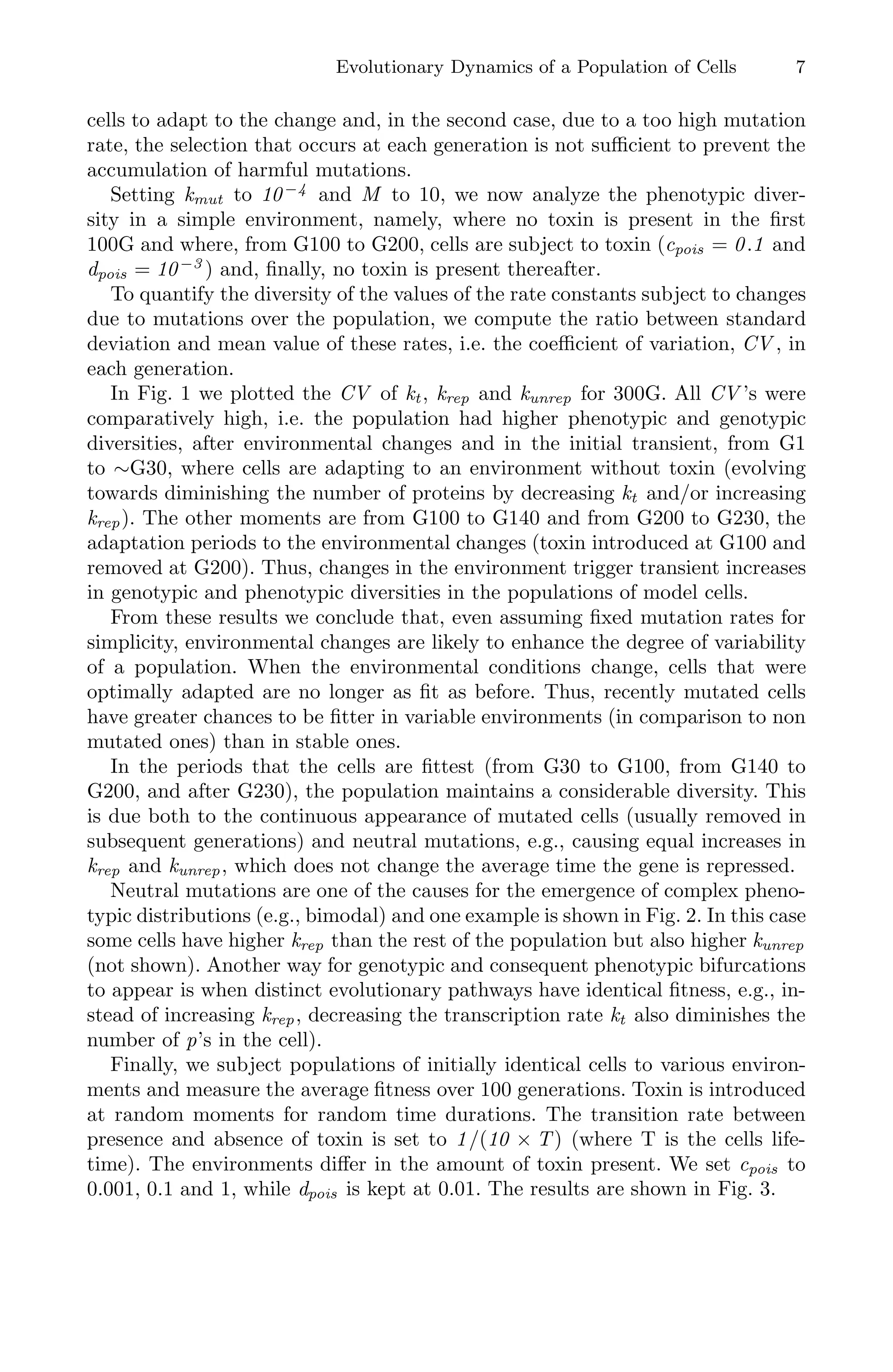
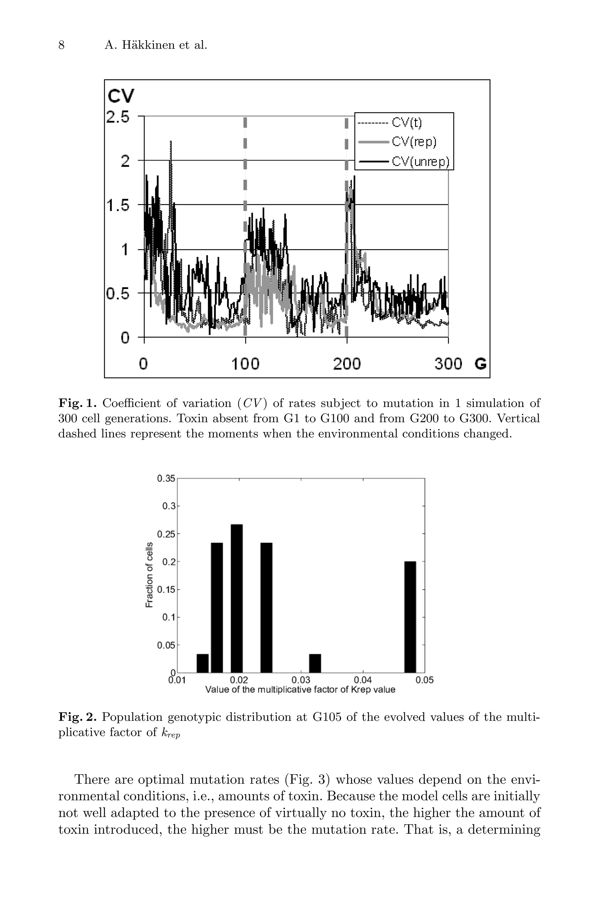
![Evolutionary Dynamics of a Population of Cells 9
Fig. 3. Average fitness in 100 G for various toxin dosages and mutation rates
factor of the value of optimal mutation rates is the necessary genotypic and phe-
notypic change to reach maximum fitness. Initially, less well-adapted cells require
higher mutation rates to rapidly create diversity from which fitter cells can be
selected from. This suggests that it is advantageous for cells to tune or evolve
mutation rates depending on the environmental conditions and shifting of these
conditions.
Two factors contribute to the existence of optimal mutation rates of this gene:
if mutation rates are too low, beneficial mutations do not occur fast enough to
improve the population’s fitness in reasonable time and, if mutation rates are
too high, selection is not sufficiently fast to prevent the accumulation of harmful
mutations.
4 Conclusions and Discussion
We implemented in model cells a stochastic model with delays of a self-repressing
gene responsible for Tetracycline resistance [10] in E. coli. We simulated pop-
ulations of cells over several generations, subjecting each cell to a stochastic
environment and providing them the ability to mutate the dynamical properties
of this genetic circuit. At the end of each generation, we selected the fittest cells.
We investigated the role and evolvability of both mean expression as well as
noise strength of this gene, as key variables in the ability of the cell to cope
with changing environmental conditions. We further studied the consequences
of subjecting the cells to fluctuating environmental conditions on the genotypic
and phenotypic diversity of the cell population over time.
Given an initially homogenous population we found that in stable environ-
ments, genotypic diversity is enhanced and then maintained at a given level
by neutral mutations that allow the cells to explore various equally beneficial,
distinct evolutionary pathways.
Environmental changes were found to be the main enhancer of genotypic diver-
sity, in agreement with observations [7]. When subject to changes in the amounts](https://image.slidesharecdn.com/1239117-250515023507-560aa707/75/Transactions-On-Computational-Systems-Biology-Xiii-1st-Edition-Antti-Hkkinen-24-2048.jpg)
![10 A. Häkkinen et al.
of toxins its subject to, the cell population not only evolves towards changing ap-
propriately the mean gene expression level, but also towards increasing genotypic
diversity in the moments following changes in the external conditions. In some
cases, cells evolved both mean expression level, as well as the noise strength,
which when increasing causes stronger phenotypic diversity.
We also allowed the evolution of the mutation rates themselves, and found
that there are optimal mutation rates whose rate depends on the amount of
toxin the cells were subject to. The higher the amount, the higher the mutation
rate, since the initial genotype of the cells was proper only for minute amounts
of toxin. Higher mutation rates allowed faster reaching of an optimal genotype,
at the cost of a higher rate of failure at the individual level, due to harmful
mutations.
We conclude that the optimal mutation rates in the model cells depend on
both the present level of adaptation of the cells, the necessary degree of change
to reach the optimal genotype, as well as the rate of change of environmental
conditions when these are unstable. We hypothesize that the ability to generate
heritable phenotypic variation [22] as well as the rate of mutation are likely to
be evolvable, selectable traits.
Finally, we note that we opted to subject the cells to approximately constant
amounts of toxin over long periods of time, and when environmental changes
occur, for those changes to be rather “abrupt” in comparison with the total
simulation time of the many cell generations. The more abrupt are the changes
in expected toxin levels, the more likely it is that a mutation occurring after that
change is beneficial in comparison with the previously optimally adapted cells.
In the future it will be of interest to test how the rate at which the change occurs
affects the results. We expect that the smoother is the environmental change the
slower is the selection for mutated cells. However, that will also allow the cell
population to maintain at all times, including during the change, a higher mean
level of fitness as the cells are more capable of adapting to the changes at the
same rhythm as these occur.
To the best of our knowledge, this work is the first view of how a delayed
stochastic model of a small genetic circuit may evolve when subject to environ-
mental changes, where the allowed mutations directly affect the kinetics of the
genetic circuit, and consequent response to the environment. This was feasible
because in the network modeled the protein interacts directly with the toxin.
This is not the common scenario, usually there are far more steps between gene
expression and interaction with the environment. There are several studies of
how perturbations in the environment may affect a population’s evolvability,
genotypic diversity, etc (see e.g. [23]). However, in general, the processes under
evolution are not explicitly modeled. Here we built on these works but, in our
model, it is explicitly accounted both the internal stochasticity of the gene’s
expression dynamics as well as the stochasticity of the environment, and also
the stochasticity of the interaction between each cell and its environment. In
the future, the use of these models may allow improving our understanding on](https://image.slidesharecdn.com/1239117-250515023507-560aa707/75/Transactions-On-Computational-Systems-Biology-Xiii-1st-Edition-Antti-Hkkinen-25-2048.jpg)

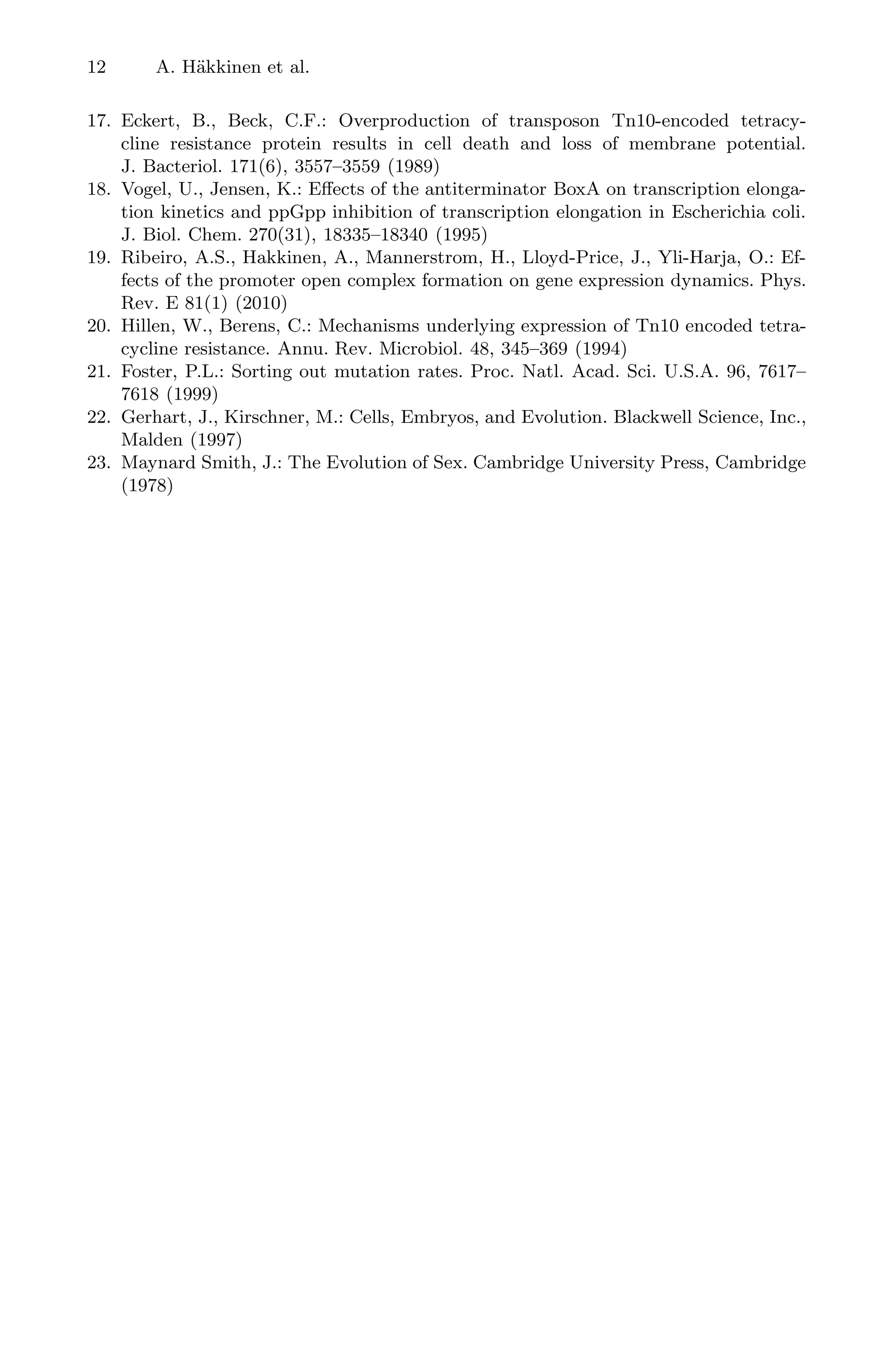
![Translation from the Quantified Implicit Process Flow
Abstraction in SBGN-PD Diagrams to Bio-PEPA
Illustrated on the Cholesterol Pathway
Laurence Loewe1
, Maria Luisa Guerriero1
, Steven Watterson1,2
,
Stuart Moodie3
, Peter Ghazal1,2
, and Jane Hillston1,3
1
Centre for System Biology at Edinburgh, King’s Buildings,
The University of Edinburgh, Edinburgh EH9 3JD, Scotland
Laurence.Loewe@ed.ac.uk, mguerrie@inf.ed.ac.uk,
2
Division of Pathway Medicine, The University of Edinburgh
S.Watterson@ed.ac.uk, P.Ghazal@ed.ac.uk
3
School of Informatics, The University of Edinburgh
Stuart.Moodie@ed.ac.uk, Jane.Hillston@ed.ac.uk
Abstract. For a long time biologists have used visual representations of bio-
chemical networks to gain a quick overview of important structural properties.
Recently SBGN, the Systems Biology Graphical Notation, has been developed to
standardise the way in which such graphical maps are drawn in order to facilitate
the exchange of information. Its qualitative Process Description (SBGN-PD) di-
agrams are based on an implicit Process Flow Abstraction (PFA) that can also be
used to construct quantitative representations, which facilitate automated analy-
ses of the system. Here we explicitly describe the PFA that underpins SBGN-PD
and define attributes for SBGN-PD glyphs that make it possible to capture the
quantitative details of a biochemical reaction network. Such quantitative details
can be used to automatically generate an executable model. To facilitate this, we
developed a textual representation for SBGN-PD called “SBGNtext” and imple-
mented SBGNtext2BioPEPA, a tool that demonstrates how Bio-PEPA models
can be generated automatically from SBGNtext. Bio-PEPA is a process algebra
that was designed for implementing quantitative models of concurrent biochem-
ical reaction systems. The scheme developed here is general and can be easily
adapted to other output formalisms. To illustrate the intended workflow, we model
the metabolic pathway of the cholesterol synthesis. We use this to compute the
statin dosage response of the flux through the cholesterol pathway for different
concentrations of the enzyme HMGCR that is inhibited by statin.
1 Introduction
Biologists are constantly searching for strategies that help them to understand the com-
plexity of life. Navigating the functional molecular interactions within cells has proven
to be an increasing challenge since molecular biological research is filling databases
with detailed knowledge about the molecular mechanics of life. A wide variety of
schemes has been developed to represent such knowledge, ranging from textual rep-
resentations that resemble chemical reactions (e.g. Dizzy [42]) or reaction rules (e.g.
C. Priami et al. (Eds.): Trans. on Comput. Syst. Biol. XIII, LNBI 6575, pp. 13–38, 2011.
c
Springer-Verlag Berlin Heidelberg 2011](https://image.slidesharecdn.com/1239117-250515023507-560aa707/75/Transactions-On-Computational-Systems-Biology-Xiii-1st-Edition-Antti-Hkkinen-28-2048.jpg)
![14 L. Loewe et al.
BioNetGen, Kappa [13,12,24]) through XML-based standards like SBML [25] to
graphical notations (e.g. [29,43,28,38,15,33]). Graphical maps of biochemical reaction
networks are proving to be powerful tools for facilitating an overview of the interactions
of particular molecules. Recently the Systems Biology Graphical Notation (SBGN) has
emerged as a standard for drawing such reaction diagrams [33,32]. The objective is to
provide molecular systems biologists with an easily understandable description of the
system by generating consistent maps across different editing tools (e.g. CellDesigner
[18], Cytoscape [11], Edinburgh Pathway Editor [46], JDesigner [44]). Like electronic
circuit diagrams, they aim to unambiguously describe the structure of a complex net-
work of interactions using graphical symbols.
To achieve this requires a collection of symbols and rules for their valid combina-
tion. The SBGN Process Description, SBGN-PD, is a visual language with a precise
grammar that builds on an underlying abstraction as the basis of its semantics (see p.40
[33]). We call this underlying abstraction for SBGN-PD the “Process Flow Abstraction”
(PFA). It describes biological pathways in terms of processes that transform elements
of the pathway from one form into another. The usefulness of an SBGN-PD description
critically depends on the faithfulness of the underlying PFA and a tight link between
the PFA and the glyphs used in diagrams. The graphical nature of SBGN-PD allows
only for qualitative descriptions of biological pathways. However, the underlying PFA
is more powerful and also forms the basis for quantitative descriptions that could be
used for analysis. Such descriptions, however, need to allow the inclusion of the corre-
sponding mathematical details like parameters and equations for computing the rate at
which reactions occur.
Here we aim to make explicit the PFA that already underlies SBGN-PD implicitly.
This serves a twofold purpose. First, a better and clearer understanding of the under-
lying abstraction will make it easier for biologists to construct SBGN-PD diagrams.
Second, the PFA is easily quantified and making this explicit can facilitate the quanti-
tative description of SBGN-PD diagrams. Such descriptions can then be used directly
for predicting quantitative properties of the system in simulations. Here we demonstrate
how this could work by mapping SBGN-PD to a quantitative analysis system. We use
the process algebra Bio-PEPA [10,3] as an example, but our mapping can be easily
applied to other formalisms as well.
This paper is an extension of previous work presented at the CompMod09 Workshop
[36]. Besides small improvements throughout the paper we provide more details on
the overall workflow that now includes a working prototype of the Edinburgh Pathway
Editor [46] and a fuller introduction to the Bio-PEPA background. Most importantly we
apply our toolchain to a completely new example with more entities than the MAPK
signalling pathway we used before. As example we now use the metabolic pathway that
produces cholesterol, which is modelled in collaboration with colleagues at the Division
of Pathway Medicine at the University of Edinburgh. We use our model to investigate
how statin inhibits cholesterol production under various circumstances – a question of
considerable medical interest [2,8,31].
The rest of the paper is structured as follows. First we provide an overview of the
implicit PFA with the help of an analogy to a system of water tanks, pipes and pumps
(Section 2). In Section 3 we explain how this system can be extended in order to capture](https://image.slidesharecdn.com/1239117-250515023507-560aa707/75/Transactions-On-Computational-Systems-Biology-Xiii-1st-Edition-Antti-Hkkinen-29-2048.jpg)
![Cholesterol Pathway: SBGN to Bio-PEPA 15
PFA : water tank
SBGN-PD: entity pool node
Bio-PEPA : species component
S P
E
PFA : pipes
SBGN-PD: consumption/production arcs
Bio-PEPA : operators
PFA : control electronics
SBGN-PD: modulating arcs
Bio-PEPA : operator + kinetic laws
PFA : pump
SBGN-PD: process
Bio-PEPA : action
S P
E
Fig. 1. An overview of the process flow abstraction. The chemical reaction at the top is translated
into an analogy of water tanks, pipes and pumps that can be used to visualise the process flow
abstraction. The various elements are also mapped into SBGN-PD and Bio-PEPA terminology.
quantitative details of the PFA. We then show how SBGN-PD glyphs can be mapped to
a quantitative analysis framework, using the Bio-PEPA modelling environment [3] as
an example (Section 4). In Section 5 we discuss various internal mechanisms and data
structures needed for translation into any quantitative analysis framework. Section 6
demonstrates the intended workflow by using a model of the cholesterol pathway as
an example. We draw a SBGN-PD map of the cholesterol pathway in the Edinburgh
Pathway Editor [46] to visualise it and to add quantitative details. The Edinburgh Path-
way Editor model can be exported as SBGNtext, which is automatically translated into
a Bio-PEPA model by our new translation tool “SBGNtext2BioPEPA” [34,35]. This
model is then investigated in the Bio-PEPA Eclipse Plugin. We end by reviewing re-
lated work and providing some perspectives for further developments.
2 The Implicit Process Flow Abstraction of SBGN-PD
The PFA behind SBGN-PD is best introduced in terms of an analogy to a system of
many water tanks that are connected by pipes. Each pipe either leads to or comes from
a pump whose activity is regulated by dedicated electronics. In the analogy, the water
is moved between the various tanks by the pumps. In a biochemical reaction system,
this corresponds to the biomass that is transformed from one chemical species into
another by chemical reactions. SBGN-PD aims to also allow for descriptions at levels
above individual chemical reactions. Therefore the water tanks or chemical species are
termed “entities” and the pumps or chemical reactions are termed “processes”. For an
overview, see Figure 1. We now discuss the correlations between the various elements
in the analogy and in SBGN-PD in more detail. In this discussion we occasionally
allude to SBGNtext, which is a full textual representation of the semantics of SBGN-PD
(developed to facilitate automated translation of SBGN-PD into other formalisms; see
[34,35]). Here are the key elements of the PFA:
Water tanks = entity pool nodes (EPNs). Each water tank stands for a different
pool of entities, where the amount of water in a tank represents the biomass that](https://image.slidesharecdn.com/1239117-250515023507-560aa707/75/Transactions-On-Computational-Systems-Biology-Xiii-1st-Edition-Antti-Hkkinen-30-2048.jpg)

![Cholesterol Pathway: SBGN to Bio-PEPA 17
pump in the analogy corresponds to the frequency with which the reaction occurs
and determines the amount of water (or biomass) that is transported between tanks
(or that is converted from one entity to another, respectively). Processes can belong
to different types in SBGN-PD (Table 2) and are unambiguously identified by a
unique ProcessNodeID in SBGNtext. This allows arcs to clearly define which
process they belong to and, by finding all its arcs, each process can also identify all
EPNs it is connected to.
Reversible processes. SBGN-PD allows for processes to be reversible if they are
symmetrically modulated (p.28 [33]). Thus, there may be flows in two directions.
However the net flow at any given time will be unidirectional. The PFA does not
prescribe how to implement this. For simplicity, our analogy assumes pumps to
be unidirectional, like many real-world pumps. Thus bidirectional processes in our
analogy are represented as two pumps with corresponding sets of pipes and oppo-
site directions of flow. In a reversible process the products of the forward process
are consumed in the backward process, thus Consumption and Production arcs
can no longer be as clearly separated as in unidirectional processes. To resolve this,
SBGN-PD distinguishes the left-hand side from the right-hand side of a process
and uses only arcs that look like Production arcs to indicate the double role (p.32
[33]). In SBGN-PD reversible process nodes are easy to recognise visually by the
absence of Consumption arcs on both sides. To represent all such arcs either as
Consumption arcs or as Production arcs in SBGNtext would lose the informa-
tion of which arc is on which side of the process node. Thus we define two new
arc types that are only used for products and reactants in the context of reversible
processes: LeftHandSide and RightHandSide.LeftHandSide arcs indicate that
they are consumption arcs in the forward process (and production arcs in the back-
ward process), where as RightHandSide arcs are the corresponding opposite. To
support reversible processes the visual editor needs to identify reversible processes
and assign the corresponding arc types LeftHandSide and RightHandSide to the
arcs. In addition a forward and a backward kinetic law need to be stored to facilitate
breaking up a bidirectional process into two unidirectional processes.
Control electronics for pumps = modulating arcs and logic gates. In the analogy,
pumps need to be regulated, especially in complex settings. This is achieved by
control electronics. In SBGN-PD, the same is done by various types of modulation
arcs, logic arcs and logic gates [33]. They all contribute to determining the fre-
quency of the reaction. Since SBGN-PD does not quantify these interactions, most
of our extensions for quantifying SBGN-PD address this aspect. Each arc con-
nects a “water tank” with a given EntityPoolNodeID and a “pump” with a given
ProcessNodeID. Ordinary modulating arcs can be of type Modulation (most
generic influence on reaction), Stimulation (catalysis or positive allosteric reg-
ulation), Catalysis (special case of stimulation, where activation energy is low-
ered), Inhibition (competitive or allosteric) or NecessaryStimulation
(process is only possible if the stimulation is “active”, i.e. has surpassed some
threshold). The glyphs are shown in Table 3, where their mapping to Bio-PEPA is
discussed. One might misread SBGN-PD to suggest that Consumption /
Production arcs cannot modulate the frequency of a process. However, kinetic](https://image.slidesharecdn.com/1239117-250515023507-560aa707/75/Transactions-On-Computational-Systems-Biology-Xiii-1st-Edition-Antti-Hkkinen-32-2048.jpg)
![18 L. Loewe et al.
Table 2. Categories of “pumps” in the process flow abstraction correspond to types of processes
in SBGN-PD. The grey lines indicate that more than one EPN can participate in this process.
SBGN-PD glyph ProcessType meaning
Process normal known processes
Association special process that builds complexes
Dissociation special process that dissolves complexes
Omitted several known processes are abstracted
Uncertain existence of this process is not clear
Observable this process is easily observable
laws frequently depend on the concentration of reactants, implying that these arcs
can also contribute to the “control electronics” (e.g. report “level of water in tank”).
Another part of the “control electronics” are logical operators. These simplify mod-
elling, when a biological function can be approximated by a simple on/off logic that
can be represented by boolean operators. SBGN-PD supports this simplification by
providing the logical operators “AND”, “OR” and “NOT”. These take “logic arcs”
as input and output, which convert a molecule count into a digital signal and back.
Groups of water tanks = compartments, submaps and more. The PFA is complete
with all the elements presented above. However, to make SBGN-PD more useful
for modelling in a biological context, SBGN-PD has several features that make it
easier for biologists to recognise various subsets of entities that are related to each
other. For example, entities that belong to the same compartment can be grouped
together in the compartment glyph and functionally related entities can be placed
on the same submap. In the analogy, this corresponds to grouping related water
tanks together. SBGN-PD also supports sophisticated ways for highlighting the in-
ner similarities between entities based on a knowledge of their chemical structure
(e.g. modification of a residue, formation of a complex). Stretching the analogy,
this corresponds to a way of highlighting some similarities between different wa-
ter tanks. These groupings are only conceptual and have no effect on quantitative
analysis, as long as different “water tanks” remain separate.
3 Extensions for Quantitative Analysis
The process flow abstraction that is implicit in all SBGN process diagrams can be used
as a basis to quantify the systems they describe. Following the introduction to the PFA
above, we now discuss the attributes that need to be added to the various SBGN-PD
glyphs in order to allow for automatic translation of SBGN-PD diagrams into quantita-
tive models. These attributes are stored as strings in SBGNtext (our textual representa-
tion of SBGN-PD, see [35]) and are attached to the corresponding glyphs by a graphical](https://image.slidesharecdn.com/1239117-250515023507-560aa707/75/Transactions-On-Computational-Systems-Biology-Xiii-1st-Edition-Antti-Hkkinen-33-2048.jpg)
![Cholesterol Pathway: SBGN to Bio-PEPA 19
SBGN-PD editor. They do not require a visual representation that compromises the vi-
sual ease-of-use that SBGN-PD aims for. A prototypic example of how the quantitative
information could be added in a visual editor is provided by the Edinburgh Pathway
Editor [46] and shown in Figure 2. Next we discuss the various attributes that are nec-
essary for the glyphs of SBGN-PD to support quantitative analysis. We do not discuss
SBGN-PD glyphs for auxiliary units, submaps, tags and equivalence arcs here, as they
do not require extensions for supporting quantitative analysis.
3.1 Quantitative Extensions of EntityPoolNodes
For quantitative analysis, each unique EPN requires an InitialMoleculeCount to
unambiguously define how many entities exist in this pool in the initial state. We fol-
lowed developments in the SBML standard in using counts of molecules instead of
concentrations, since SBGN-PD also allows for multiple compartments, making the
use of concentrations very cumbersome (see section 4.13.6, p.71f. in [25]). For entities
of type Perturbation, the InitialMoleculeCount is interpreted as the numerical
value associated with the perturbation, even though its technical meaning is not a count
of molecules. Entities of the type Source or Sink are both assumed to be effectively
unlimited, so InitialMoleculeCount does not have a meaning for these entities. Be-
yond a unique EntityPoolNodeID and InitialMoleculeCount, no other informa-
tion on entities is required for quantitative analysis.
3.2 Quantitative Extensions of Arcs
Arcs link entities and processes by storing their respective IDs and the ArcType. The
simplest arcs are of type Consumption or Production and do not require numerical
information beyond the stoichiometry that is already defined in SBGN-PD as a property
of arcs that can be displayed visually in standard SBGN-PD editors. Logic arcs will be
discussed below. All modulating arcs are part of the “control electronics” and affect the
frequency with which a process happens. They link to EPNs to inform the process about
the presence of enzymes, for example. Modulation is usually governed by parameters
or other important quantities for the given process (e.g. Michaelis-Menten constant).
To make the practical encoding of a model easier, we define process pa-
rameters that conceptually belong to a particular modulating entity as a list of
QuantitativeProperties in the arc pointing to that entity. This is equivalent to see-
ing the set of parameters of a reaction as something that is specific to the interaction
between a particular modulator and the process it modulates. Other approaches are also
possible, but lead to less elegant implementations. Storing parameters in equations re-
quires frequent and possibly error-pronechanges (e.g. many different Michaelis-Menten
equations). One could also argue that the catalytic features are a property of the enzyme
and thus make parameters part of EPNs; however this would mean that all the reac-
tions catalysed by the same enzyme would have the same parameters or would require
cumbersome naming conventions to manage different affinities for different substrates.
To refer to parameters we specify the ManualEquationArcIDof an arc and then the
name of the parameter that is stored in the list of QuantitativeProperties of that
arc. This scheme reduces clutter by limiting the scope of the relevant namespace (only
few arcs per process exist, so ManualEquationArcIDs only need to be unique within](https://image.slidesharecdn.com/1239117-250515023507-560aa707/75/Transactions-On-Computational-Systems-Biology-Xiii-1st-Edition-Antti-Hkkinen-34-2048.jpg)
![20 L. Loewe et al.
A
B
Fig. 2. An example of how attributes attached to SBGN-PD glyphs and stored as strings can be
used to add quantitative information to a visual representation of a biochemical reaction network.
These screenshots from the Edinburgh Pathway Editor (Version 3.0.0-alpha13) [46] show a se-
lected glyph with its attributes that are automatically displayed in the properties window. (A)
EntityPoolNode “Entity Count” is mapped to InitialMoleculeCount. (B) ProcessNode with
attributes for entering the propensity functions for the forward and backward reactions. “Export
Name” facilitates the production of readable Bio-PEPA models.
that immediate neighbourhood). Thus parameter names can be brief, since they only
need to be unique within the arc. The ManualEquationArcID is specified by the user
in the visual SBGN-PD editor and differs from ArcID, a globally unique identifier that
is automatically generated by the graphical editor. The ManualEquationArcID allows
for user-defined generic names that are easy to remember, such as “Km” and “vm” for
Michaelis-Menten reactions. It should be easily accessible within the graphical editor,
just as the parameters that are stored within an arc.
Logical operators and logic arcs. To facilitate the use of logical operators in quantitative
analyses one needs to convert the integer molecule counts of the involved EPNs to
binary signals amenable to boolean logic. Thus SBGNtext supports “incoming logic
arcs” that connect a “source entity” or “source logical result” with a “destination logic
operator” and apply an “input threshold” to decide whether the source is above the
threshold (“On”) or below the threshold (“Off”). To this end, a graphical editor needs
to support the “input threshold” as a numerical attribute that the user can enter; all other
information recorded in incoming logic arcs is already part of an SBGN diagram. Once
all signals are boolean, they can be processed by one or several logical operators, until
the result of this operation is given in the form of either 0 (“Off”) or 1 (“On”). This
result then needs to be converted back to an integer or float value that can be further
processed to compute process frequencies. Thus a graphical editor needs to support
corresponding attributes for defining a low and a high output level.](https://image.slidesharecdn.com/1239117-250515023507-560aa707/75/Transactions-On-Computational-Systems-Biology-Xiii-1st-Edition-Antti-Hkkinen-35-2048.jpg)
![Cholesterol Pathway: SBGN to Bio-PEPA 21
3.3 Quantitative Extensions of ProcessNodes
For quantitative analyses, a ProcessNode must have a unique name and a kinetic law
that represents the propensity, which is proportional to the probability that this process
occurs next in a stochastic model, based on the current global state of the model. In a
deterministic model this equation gives a rate law that is expressed in terms of abso-
lute molecule numbers, not concentrations. Since the ProcessType is not required for
quantitative analyses, it does not matter whether a process is an ordinary Process,
an Uncertain process or an Observable process, for example. For all these Pro-
cessNodes, graphical editors need to support attributes for the manual specification of
a ProcessNodeID, and a PropensityFunction. These attributes are then stored in
SBGNtext. If support for bidirectional processes is desired, then graphical editors need
to facilitate entering a propensity function for the backward process as well. Propensity
functions compute the propensity of a unidirectional process to be the next event in the
model and can be used directly by simulation algorithms and ODE solvers [20].
A PropensityFunction can be given directly (see current prototype of Edinburgh
Pathway Editor [46]; Figure 2), but the full definition of SBGNtext specifies propen-
sities by referring to aliases. This can simplify the specification of models and hence
reduce errors. For instantiation, a translator needs to replace all aliases by their true
identity. We use the following syntax for a parameter alias that is substituted by the
actual numeric value (or a globally defined parameter) from the corresponding arc:
par: ManualEquationArcID.QuantitativePropertyName
While translating to Bio-PEPA this would be simply substituted with a corresponding
parameter name. The parameter is then defined elsewhere in the Bio-PEPA model to
have the numerical value stored in the corresponding property of the arc. To allow the
numerical analysis tool to access an EPN count at runtime we replace the following
entity alias by the EntityPoolNodeID that the corresponding arc links to:
ent: ManualEquationArcID
This is shorter than the EntityPoolNodeID and allows the reuse of propensity func-
tions if kinetic laws are identical and the manual IDs follow the same pattern. It is
desirable that there is no need to specify the EntityPoolNodeID since it is fairly long
and generated automatically to reflect various properties that make it unique. It would
be cumbersome to refer to in the equation and it would require a mechanism to access
the automatically generated EntityPoolNodeID before a SBGNtext file is generated.
Also any changes to an entity that would affect its EntityPoolNodeIDwould then also
require a change in all corresponding propensity functions, a potentially error-prone
process. The same substitution mechanism can be used to provide access to proper-
ties of compartments (see [35]). In addition to these aliases, functions use the typical
standard arithmetic rules and operators that are directly passed through to the next level.
4 Mapping SBGN-PD Elements to Bio-PEPA
In this section we explain how to use the semantics of SBGN-PD to map a SBGN-PD
model to a formalism for quantitative analysis. We are using Bio-PEPA as an example,](https://image.slidesharecdn.com/1239117-250515023507-560aa707/75/Transactions-On-Computational-Systems-Biology-Xiii-1st-Edition-Antti-Hkkinen-36-2048.jpg)
![22 L. Loewe et al.
but our approach is general and can be applied to many other formalisms that support
the modelling of chemical reactions.
4.1 The Bio-PEPA Language
Bio-PEPA is a stochastic process algebra which models biochemical pathways as inter-
actions of distinct entities representing reactions of chemical species [10,3]. A process
algebra model captures the behaviour of a system as the actions and interactions be-
tween a number of entities, where the latter are often termed “processes”, “agents” or
“components”. In PEPA [23] and Bio-PEPA [10] these are built up from simple se-
quential components. Different process algebras support different modelling styles for
biochemical systems [5]. Stochastic process algebras, such as PEPA [23] or the stochas-
tic π-calculus [41], associate a random variable with each action to represent the mean
of its exponentially distributed waiting time. In the stochastic π-calculus, interactions
are strictly binary whereas in Bio-PEPA the more general multiway synchronisation is
supported. Bio-PEPA is based on the following underlying principles (see [10] for more
details):
– modelling follows the “reagent-centric” style, which means that different species
components denote different types of reagents;
– only irreversible reactions are considered: reversible reactions can be seen as the
union of a pair of forward and backward reactions;
– the reactants of the reaction can only decrease their concentration, the products can
only increase it, whereas enzymes and inhibitors do not change;
– a single species in different states (e.g. phosphorylated, free, bound ligand, in dif-
ferent compartments, ...) is regarded as different species and represented by distinct
sequential components;
– compartments are static and do not play an active role in reactions, but they can
be used to constrain reaction occurrences to a particular location and propensity
functions can depend on their size. Here for the sake of simplicity, we assume all
species are located in the same compartment.
The syntax of Bio-PEPA is defined as [10] :
S ::= (α, κ) op S | S + S | C P ::= P
L
P | S (x)
where S is a sequential species component that represents a chemical species (termed
“process” in some other process algebras and “EntityPoolNode” in SBGN-PD), C is a
name referring to a species component defined as C ≡ S , P is a model component that
describes the set L of possible interactions between species components (these “interac-
tions” or “actions” correspond to “processes” in SBGN-PD and can represent chemical
reactions). An initial count of molecules or a concentration of S is given by x ∈ R+
0 . In
the prefix term “(α, κ) op S ”, κ is the stoichiometry coefficient and the operator op indi-
cates the role of the species in the reaction α. Specifically, op = ↓ denotes a reactant,
↑ a product, ⊕ an activator, an inhibitor and a generic modifier, which indicates
more generic roles than ⊕ or . The operator “+” expresses a choice between possible
actions. Finally, the process P
L
Q denotes the synchronisation between components:](https://image.slidesharecdn.com/1239117-250515023507-560aa707/75/Transactions-On-Computational-Systems-Biology-Xiii-1st-Edition-Antti-Hkkinen-37-2048.jpg)
![Cholesterol Pathway: SBGN to Bio-PEPA 23
the set L determines those activities on which the operands are forced to synchronise.
When L is the set of common actions, we use the shorthand notation P
∗
Q. A Bio-
PEPA model P is defined as a 6-tuple V, N, K, FR,Comp, P , where: V is the set of
compartments, N is the set of quantities describing each species, K is the set of all pa-
rameters referenced elsewhere, FR is the set of functional rates that define all required
kinetic laws, Comp is the set of definitions of species components S that highlight the
reactions a species can take part in and P is the system model component.
A variety of analysis techniques can be applied to a single Bio-PEPA model, facilitat-
ing the easy validation of analysis results when the analyses address the same issues [4]
and enhancing insight when the analyses are complementary [9,1]. Currently supported
analysis techniques include stochastic simulation at the molecular level, ordinary dif-
ferential equations, probabilistic and statistical model-checking and numerical analysis
of continuous time Markov chains [10,3,17]. Additional analysis techniques are facili-
tated by compositional reasoning, which allows the automated extension of elementary
proofs of qualitative features to complex models. Examples for such qualitative analy-
ses include deadlock and livelock detection and model-checking of a model against a
logical formula.
4.2 SBGN-PD Mapping
Here we map the core elements of SBGN-PD to Bio-PEPA (see [34] for an implemen-
tation).
Entity Pool Nodes. Due to the rich encoding of information in the EntityPoolNode-
ID, Bio-PEPA can treat each distinct EntityPoolNodeID as a distinct species com-
ponent. This removes the need to explicitly consider any other aspects such as entity
type, modifications, complex structures and compartments, as all such information is
implicitly passed on to Bio-PEPA by using the EntityPoolNodeID as the name for
the corresponding species component. The definition of the set N of a Bio-PEPA sys-
tem requires the attribute InitialMoleculeCount for each EPN (see Section 3).
Processes. All SBGN-PD ProcessTypes are represented as reactions in Bio-PEPA.
Compiling the corresponding set FR relies on the attribute PropensityFunction and
a substitution mechanism that makes it easy to define these functions manually. To help
humans understand references to processes in the sets FR and Comp requires recog-
nisable names for SBGN-PD ProcessNodeIDs that map directly to their identifiers in
Bio-PEPA. Thus graphical editors need to support manual ProcessNodeIDs.
Reversible processes. The translator supports reversible SBGN-PD processes by di-
viding them into two unidirectional processes for Bio-PEPA. The translator reuses the
manually assigned ProcessNodeID and augments it by “ F” for forward reactions
and “ B” for backward reactions. These two unidirectional processes are then treated
independently. When compiling the species components in Bio-PEPA, every time a
LeftHandSide arc is found, the translator assumes that the corresponding forward
and backward processes have been defined and will augment the process name appro-
priately, while adding the corresponding Bio-PEPA operator for reactant and product.](https://image.slidesharecdn.com/1239117-250515023507-560aa707/75/Transactions-On-Computational-Systems-Biology-Xiii-1st-Edition-Antti-Hkkinen-38-2048.jpg)
![24 L. Loewe et al.
Table 3. “Water pipes and control electronics”: Mapping arcs between entities and processes in
SBGN-PD to operators in Bio-PEPA species components. “Symbols” are the formal syntax of
Bio-PEPA, while “code” gives the concrete syntax used in the Bio-PEPA Eclipse Plug-in [3].
SBGN-PD glyph ArcType Bio-PEPA symbol Bio-PEPA code
Consumption ↓
Production ↑
LeftHandSide ↓ and ↑ and
RightHandSide ↑ and ↓ and
Modulation (.)
Stimulation ⊕ (+)
Catalysis ⊕ (+)
Inhibition (-)
NecessaryStimulation (.)
RightHandSide arcs are handled in the same way. Thus the production arc glyph in
SBGN-PD has three distinct meanings as shown in Table 3.
Arcs. The arcs in SBGN-PD define which entities participate in which processes. Thus
arcs play a pivotal role in defining the species components in Bio-PEPA. Since arcs can
store kinetic parameters, they are also important for defining parameters in Bio-PEPA.
As kinetic law definitions in Bio-PEPA frequently refer to such parameters, we use
the ArcID that is automatically generated by the graphical editor to substitute the local
manual arc references in propensity functions by globally unique parameters names
(see Section 3). The type of an arc indicates both the role of the connected entity in the
process (consumed reactant, product or rate modifier) and the chemical nature of the
reaction (catalysis, stimulation, inhibition, necessary stimulation or the most generic
modification). Thus the type of an arc can be mapped directly to the operator “op”
described in the Bio-PEPA syntax shown in Table 3. All mappings are straightforward
except NecessaryStimulation (previously called Trigger), which we mapped to
the generic modifier to indicate that this interaction inhibits below and stimulates
above a given threshold.
Logical operators. Logical operators require the conversion of integer molecule counts
of the relevant EPNs to binary signals and after some boolean logic processing back to
low and high integer values. As evident from the implementation scheme above, the use
of all quantitative properties culminates in the correct formulation of the corresponding
propensity functions that determine the probability that the corresponding process will
be the next to occur. Thus an implementation of logical operators requires that their
results be included in the corresponding propensity functions. The current scheme of
implementing propensity functions relies heavily on substituting the various compo-
nents into the final equation, so that Bio-PEPA will ultimately only see one formula per](https://image.slidesharecdn.com/1239117-250515023507-560aa707/75/Transactions-On-Computational-Systems-Biology-Xiii-1st-Edition-Antti-Hkkinen-39-2048.jpg)
![Cholesterol Pathway: SBGN to Bio-PEPA 25
propensity function. In this context the implementation of logical operators requires the
insertion of a formula in the propensity function that computes the result of the boolean
operations from their integer input. An arbitrarily complex logic operator network can
be constructed from the following basic building blocks:
– Convert from integers or double floats to boolean values. This is best done by a
specially defined mathematical function that takes an integer or float signal and
compares it to a specified threshold, returning either 0 (signal ≤ threshold) or 1
(signal threshold). The definition of such a function is not complicated and can
be implemented with the help of the Heaviside step function that is available in the
Bio-PEPA Eclipse Plug-in.
– Map boolean operators: AND → multiply all boolean inputs to get output. NOT
→ use the arithmetic expression output = (1 − input). OR → sum all inputs (0/1)
and test if it is greater than 1 using the threshold function.
5 Converter Implementation and Internal Representation
We chose Java as implementation language for the converter described above, due to
the good portability of the resulting binaries and for interoperability with the Bio-PEPA
Eclipse Plug-in [3]. We defined a grammar for SBGNtext in the Extended Backus-
Naur-Form (EBNF) as supported by ANTLR [39], which automatically compiles the
Java sources for the parser that stores all important parsing results in a number of co-
herently organised internal TreeMaps. To generate a Bio-PEPA model three main loops
over these TreeMaps are necessary: over all entities, over all processes and over all
parameters. To illustrate the translation we refer to “code” examples from Figure 3.
The loop over all entities (e.g. “m LSS Ent”) compiles the species components as
well as the model component required by Bio-PEPA. The latter is a list of all partici-
pating EntityPoolNodeIDs combined by the cooperation operator “ ∗ ” or
∗
that
automatically synchronises on all common actions (“∗”). This simplification depends
on all processes in SBGN-PD having unique names and fixed lists of reactants with
no mutually exclusive alternatives in them. The first condition can be enforced by the
tools that produce the code, the second is ensured by the reaction-style of describing
processes in SBGN-PD. For example, SBGN-PD does not allow for a single reaction
called “bind”, which states that A binds with either B or C to produce D. In Bio-PEPA
these alternative reactions could be given the same name and careful construction of
the model equation could then ensure that only one of B or C participates in any one
occurrence of the reaction. To describe the same model in SBGN-PD requires two reac-
tions with different names (A+B→D; A+C→D;). This is then translated into the correct
Bio-PEPA model using only “ ∗ ”. Hence individual actions synchronised by the
cooperation operator do not need to be tracked in this system.
For each species component a loop over all arcs finds the arcs that are connected
to it (e.g. “st33”) and that store all relevant ProcessNodeIDs (e.g. “LSS Proc”). The
same loop determines the respective role of the component (as reflected by the choice
of the Bio-PEPA operator in Table 3; e.g. “(+)”). To compile this we loop over all
arcs to find the arcs that connect to a particular entity. Since the arc also contains the](https://image.slidesharecdn.com/1239117-250515023507-560aa707/75/Transactions-On-Computational-Systems-Biology-Xiii-1st-Edition-Antti-Hkkinen-40-2048.jpg)
![26 L. Loewe et al.
... // header
EntityPoolNode m_LSS_Ent {
EPNName = LSS ;
EPNType = Macromolecule ;
EPNState = { } ;
InitialMoleculeCount = 10000 ;
} ... // more EPNs
ProcessNode LSS_Proc {
ProcessType = Process;
PropensityFunction =
par: enz.kcat*ent: enz*ent: subs
/ (par: enz.Km_CountCell + ent: subs) ;
} ... // more ProcessNodes
Arc st33 {
ManualEquationArcID = enz ;
ArcType = Stimulation ;
Entity = m_LSS_Ent ;
Process = LSS_Proc ;
Stoichiometry = 1 ;
QuantitativeProperties = {
( Km_CountCell = 0.015 * omega )
( kcat = 1000.0 )
} ;
} ... // more Arcs
... // ending
st33_Km_CountCell = 0.015 * omega;
st33_kcat = 1000.0;
... // more parameters
kineticLawOf LSS_Proc :
st33_kcat * m_LSS_Ent
* m_23oxydosqualene_Ent
/ ( st33_Km_CountCell *
m_23oxydosqualene_Ent )
; ... // more kinetic laws
m_LSS_Ent =
( LSS_Proc , 1 ) (+) m_LSS_Ent
; ... // more species components
// model component with initial counts per cell
m_LSS_Ent [10000] *
m_23oxydosqualene_Ent[0] * ...
// more species components [initial count]
SBGNtext
Bio-PEPA
SBGN
Process
Description
2,3-oxydosqualene
LSS
lanosterol
Fig. 3. Transformation of biochemical reaction systems in the automated workflow from
SBGN-PD to Bio-PEPA. Using an extract of the cholesterol pathway model discussed below,
this example shows how parts from one representation are transformed into parts of another. The
code excerpts focus on the enzyme (“LSS Proc”) and the reaction it catalyses (“LSS Proc”). Pa-
rameters such as kinetic constants and initial amounts of species must be scaled from the start in
the Edinburgh Pathway Editor to represent discrete molecule counts.
process ID and no further information about a process is required here, there is no
need to loop over all processes as well. By combining the information stored in the
TreeMaps of entities and arcs, it is possible to compile the relevant information for Bio-
PEPA species components. The fact that multiple arcs can connect the same entity to
multiple reactions and the same reaction to multiple entities facilitates the preservation
of SBGNs capacity to model reactions with many entities during the translation process.
The loop over all processes (e.g. “LSS Proc”) compiles the kinetic laws by substi-
tuting aliases (e.g. “ent: enz” or “par: enz.kcat” ) for EPNs (“m LSS Ent”)
and parameters (“st33 kcat”) in the propensity functions specified in the graphical
editor. Each function is handled separately by a dedicated function parser that queries
the TreeMaps generated when parsing the SBGNtext file.1
1
Our prototypic implementation of the workflow presented here passes propensity functions
entered in the Edinburgh Pathway Editor without modification to Bio-PEPA. A version of
SBGNtext2BioPEPA that substitutes parameters in functions is available from [34].](https://image.slidesharecdn.com/1239117-250515023507-560aa707/75/Transactions-On-Computational-Systems-Biology-Xiii-1st-Edition-Antti-Hkkinen-41-2048.jpg)
![Cholesterol Pathway: SBGN to Bio-PEPA 27
The loop over all quantitative properties of the model defines the parameters in
Bio-PEPA (e.g. “st33 kcat”). It is possible to avoid this step by inserting the direct
numerical values into the equations processed in the second loop. However, this sub-
stantially reduces the readability of equations in the Bio-PEPA model and makes it
difficult for third party tools to assist in the automated generation of parameter com-
binations. Thus we defined a scheme that automatically generates parameter names to
maximise the readability of equations (combine ArcID “st33” and name of the quanti-
tative property “kcat”).
To facilitate walking through the various collections specified above, the TreeMaps
are organised in four sets, one set for entities, one for processes, one for arcs and one for
quantitative properties. Each of these sets is characterised by a common key to all maps
within the set. This facilitates the retrieval of related parse products for the same key
from a different map. Since all this information is accessible from Java code, it is easily
conceivable to use the sources produced in this work for reading SBGNtext files in a
wide variety of contexts. The system is easy to deploy, since it involves few files and the
highly portable ANTLR runtime library. Our converter is called SBGNtext2BioPEPA
and sources are available [34].
6 Example: Competitive Inhibition in the Cholesterol Pathway
6.1 A Model of the Cholesterol Synthesis Pathway
Here we illustrate our translation workflow by using the cholesterol synthesis pathway
as an example. We first draw an SBGN-PD map of this pathway (Figure 4) in the Ed-
inburgh Pathway Editor (EPE) [46] based on the biochemical reactions listed in KEGG
[27]. Then we add the necessary quantitative extensions as attributes to the correspond-
ing glyphs in EPE (for screenshot see Figure 2), before we export the model from
EPE to SBGNtext. SBGNtext is automatically translated to Bio-PEPA with the help
of SBGNtext2BioPEPA [34]. Finally the model is simulated in the Bio-PEPA Eclipse
Plugin Version 0.1.7 [3] using the Gibson-Bruck stochastic simulation method [19]
and the Adaptive Dormant Prince ODE solver. Fluxes are computed from the exported
time courses as described below. Since our model is focussed on the flux of de novo
cholesterol production, we choose to ignore the complex processes that degrade or store
cholesterol.
Scaling of the System. Since Bio-PEPA and SBML [25] describe systems in terms of
explicit molecule counts and not concentrations, we introduce a scaling factor Ω which
is used to represent the size of the system. The factor Ω effectively converts a concentra-
tion [mM] into a molecular count by multiplying it with Avogadro’s number and a vol-
ume. As a volume we cannot use the typical volume of a cell, since cholesterol synthesis
is confined to the endoplasmatic reticulum, which comprises only a fraction of the cell.
At this stage we do not have information about the volume of a cell dedicated to choles-
terol synthesis. However, rough estimates show that many typical enzymes that are not
produced in particularly high copy numbers exist in about 104
copies / cell. Thus we](https://image.slidesharecdn.com/1239117-250515023507-560aa707/75/Transactions-On-Computational-Systems-Biology-Xiii-1st-Edition-Antti-Hkkinen-42-2048.jpg)
![28 L. Loewe et al.
acetyl-CoA
HMGCS1
HMG-CoA
HMGCR
mevalonate
MVK
mevalonate-5P
PMVK
mevalonate-5PP
MVD
isopentyl-PP
EUPPS
farnesyl-PP
FDFT1
squalene
CYP51A1
4,4-dimethyl-cholestra-8,14,24-trienol
SQLE
2,3-oxydosqualene
LSS
lanosterol
GGPS FDPS
TM7SF2
14-demethyl-lanosterol
NSDHL
3-keto-4-methyl-zymosterol
HSD17B7
4-methyl-zymosterol
zymosterol
desmosterol
7-dehydro-desmosterol
SC4MOL
4-methyl-zymosterol-carboxalate
cholestra-7,24-dien-3beta-ol
cholesterol
DHCR24
cholestra-8,en-3beta-ol
EBP
lathosterol
SC5DL
7-dehydro-cholesterol
DHCR7
statin
Fig. 4. A SBGN-PD representation of the cholesterol pathway as taken from KEGG [27], drawn
in the Edinburgh Pathway Editor [46]. Metabolites are marked as yellow to highlight the mostly
linear structure of the pathway. Enzymes are coloured in cyan and the inhibitory statin in red. A
constant flow of acetyl-CoA is assumed to enter the system.
choose Ω such that a 10 mM enzyme concentration translates into 10000 copies / cell
(Ω = 1000), giving our model a realistic scale. Explicitly representing Ω increases the
flexibility of the model by allowing quick changes to the size of the system2
.
2
Since parameters cannot be defined explicitly in the current EPE prototype, we model Ω as
a “dummy-species”, that does not take part in reactions, but has a constant value, which can
be referred to in propensity functions for the purpose of scaling KM. Since the initial “Entity
Count” needs to be an integer of the right size we enter 10000 directly (= 10 · Ω).](https://image.slidesharecdn.com/1239117-250515023507-560aa707/75/Transactions-On-Computational-Systems-Biology-Xiii-1st-Edition-Antti-Hkkinen-43-2048.jpg)
![Cholesterol Pathway: SBGN to Bio-PEPA 29
Table 4. Kinetic parameters for Michaelis-Menten reactions as used in our model. Values for the
reaction rate parameters were taken from BRENDA [7] where possible. In order to have units
uniformly in terms of molecule counts, KM needs to be multiplied with the system size Ω that is
also used to specify the enzyme count (see as in Eq.1). Values marked with “*” are hypothetical.
Reactions not listed here are assumed to follow mass action kinetics with rate constants of 1000
(reactants: 4-methyl-zymosterol, cholestra-7,24-dien-3β-ol, 7-dehydro-desmosterol) or {0.05, 50}
× 10 Ω (product: acetyl-CoA).
Enzyme Enzyme count Turnover kcat [1/h] KM [mM]
HMGCS1 10 Ω * 1000 * 0.01
HMGCR {3, 10, 30} Ω * 500 * 0.07
MVK 10 Ω * 1000 * 0.024
PMVK 10 Ω * 36720 0.025
MVD 10 Ω * 17640 0.0074
EUPPS 10 Ω * 1000 * 0.01 *
GGPS 10 Ω * 1000 * 0.01 *
FDPS 10 Ω * 1000 * 0.01 *
FDFT1 10 Ω * 1908 0.0023
SQLE 1000 Ω * 65.88 0.0077
LSS 10 Ω * 1000 * 0.015
CYPY1A1 10 Ω * 1000 * 0.005
TM7SF2 10 Ω * 1000 * 0.0333
SC4MOL 10 Ω * 1000 * 0.01 *
NSDHL 10 Ω * 1000 * 0.007
HSD17B7 1000 Ω * 177.48 0.236
DHCR24 - zymosterol 10 Ω * 1000 * 0.037
DHCR24 - desmosterol 10 Ω * 1000 * 0.01 *
EBP - cholestra-8,en3β-ol 10 Ω * 5122.8 0.01 *
EBP - zymosterol 10 Ω * 1522.8 0.05
SC5DL 10 Ω * 1000 * 0.032
DHCR7 10 Ω * 1000 * 0.277
Reaction Kinetics. Our typical kinetic law (propensity function for stochastic simula-
tions; rate law for ODE) for standard Michaelis Menten kinetics as entered in EPE is
kcat · EnzymeName Ent · m S ubstrateName Ent
(KM · Ω) + m S ubstrateName Ent
(1)
This function is used to model all reactions that involve one enzyme and one metabo-
lite. To do this we retrieved kinetic parameter values from BRENDA [7]. If no kinetic](https://image.slidesharecdn.com/1239117-250515023507-560aa707/75/Transactions-On-Computational-Systems-Biology-Xiii-1st-Edition-Antti-Hkkinen-44-2048.jpg)
![30 L. Loewe et al.
parameter was found for an enzyme, we assumed a turnover of kcat=1000 [1 / h] and
a Michaelis-Menten constant of KM=0.01 [mM], which is of the same order of mag-
nitude as the mean of corresponding values of other enzymes that have been observed
in experiments. Table 4 reports all relevant parameters used in our model. The reaction
catalysed by HMGCR has been described as a rate limiting step of the cholesterol path-
way [30,37]. To capture this notion in our model we increase the enzyme copy numbers
for SQLE and HSD17B7, two slow reactions for which both kcat and KM are known.
For reactions without an enzyme in Figure 4 we assumed mass action kinetics. We
chose rates so that they would not be limiting in this system and would not force the
accumulation of large amounts of reactants (see Table 4).
The first mass action reaction is special since it determines the flux of acetyl-CoA
into the system. In the absence of degradation reactions for intermediate metabolites
and the endproduct cholesterol, the influx determines the rate of cholesterol production
– unless intermediate metabolites accumulate (see below). We chose to model two sce-
narios: a low-flux scenario that represents situations where acetyl-CoA in the cell is di-
rected away from cholesterol synthesis and a high-flux scenario that reflects conditions
of more abundant acetyl-CoA. In the low and high flux scenarios 500 = 0.05 · 10 Ω and
500000 = 50 · 10 Ω molecules of acetyl-CoA are introduced into the system, respec-
tively (10 Ω was chosen to be of the same order of magnitude as the typical number of
copies per enzyme).
In order to model competitive inhibition by statin we use the following kinetic law:
kcat · EnzymeName Ent · m S ubstrateName Ent
m S ubstrateName Ent + (KM · Ω) · (1 + m InhibitorName Ent/(Ω · KI))
(2)
where HMGCR is the enzyme, HMG-CoA the metabolite, statin the inhibitor and
KI = 0.000044 [mM] the inhibition constant average of 11 values for human cells found
in BRENDA; values for other reactions are given in Table 4 . From the nature of this
function it follows that any number of inhibitor molecules can be rendered ineffective,
if countered by a sufficiently large number of metabolites (see results below).
Measurement of Cholesterol Flux. Due to the linear structure of the pathway, its uni-
directional flow and the lack of degradation of intermediate products, a steady flow
of acetyl-CoA leads to a steady production of cholesterol. If the rate of an intermedi-
ate reaction is too low, the production of cholesterol is slowed down temporarily until
the substrate of the reaction has accumulated enough to compensate for the reduction.
A simulation in the high flux environment without statin and for HMGCR = 30000
showed that all intermediates equilibrate after less than 5 minutes and then fluctuate
around fairly low molecule counts (most around zero, all below 500). To facilitate mea-
surements of cholesterol production flux F, we omitted cholesterol degrading reactions.
Instead we compute F, the flux of newly synthesised molecules of cholesterol / hour as
F =
CT2
− CT1
T2 − T1
(3)
where C represents accumulated counts of synthesised cholesterol molecules in the
system at the corresponding points T1 and T2 and time is measured in hours.](https://image.slidesharecdn.com/1239117-250515023507-560aa707/75/Transactions-On-Computational-Systems-Biology-Xiii-1st-Edition-Antti-Hkkinen-45-2048.jpg)
![Cholesterol Pathway: SBGN to Bio-PEPA 31
0
1x10⁵
2x10⁵
3x10⁵
4x10⁵
5x10⁵
6x10⁵
cholesterol
flux
[molecules
/
hour]
HMGCR = 3000
HMGCR = 10000
HMGCR = 30000
0.0
100.0
200.0
300.0
400.0
500.0
1 10 100 1000 104
105
106
107
cholesterol
flux
[molecules
/
hour]
statin molecules in the system
HMGCR = 3000
HMGCR = 10000
HMGCR = 30000
A
B
Fig. 5. Response of cholesterol flux to different amounts of statin molecules in the system. (A)
Assuming a high influx of acetyl-CoA as computed by the Adaptive Dormant Prince ODE solver
predicts mean expected values. This approximation works well for large molecule counts. (B)
Assuming a low influx of acetyl-CoA as computed by the Gibson-Bruck stochastic simulator
shows the variability associated with low copy numbers of molecules. Values were computed
by the the Bio-PEPA Plugin 0.1.7 and report the average of five runs with error bars denoting
standard deviations. We deliberately avoided averaging over many more repeats to highlight the
stochastic nature of the system.](https://image.slidesharecdn.com/1239117-250515023507-560aa707/75/Transactions-On-Computational-Systems-Biology-Xiii-1st-Edition-Antti-Hkkinen-46-2048.jpg)
![32 L. Loewe et al.
200
250
300
350
400
450
1 10 100 1000 10000 100000 1000000
cholesterol
flux
IC50
[molec.
/
hour]
HMGCR molecules
Fig. 6. The stochastic variability of the flux of cholesterol for a wide range of enzyme copy
numbers with a corresponding number of inhibitory statin molecules as given below. The higher
flux for 1 and 3 HMGCR molecules is caused by rounding off fractions computed by equation
(4) to get molecule counts. Error bars denote standard deviations observed in 50 stochastic runs,
measuring flux in the last hour of 2h simulations, as computed by the Gibson-Bruck stochas-
tic simulator. The number of statin molecules used in the simulations shown here for a given
HMGCR count were computed by rounding the result of equation (4). This resulted in the fol-
lowing HMGCR → statin pairs: 1 → 0; 3 → 1; 10 → 6; 30 → 18; 100 → 62; 300 → 188; 1000
→ 628; 3000 → 1885; 1 × 10⁴
→ 6285; 3 × 10⁴
→ 18857; 1 × 10⁵
→ 62857; 3 × 10⁵
→ 188571;
1 × 10⁶
→ 628571.
Visual inspection of all time courses with only 1 statin molecule present indicates
that the cholesterol increase follows a straight line almost immediately from the start.
This is confirmed by comparisons between the fluxes measured over the first and last
quarter of the first hour simulated in ODEs which differ by less than 5%, a difference
that is exceeded by the stochastic noise in the low-flux system. For stochastic simu-
lations, measuring flux over a whole hour integrates more events leading to less vari-
ance than measuring shorter intervals. Thus we report as F the number of cholesterol
molecules synthesised in the first hour after starting the simulation with all metabo-
lites at zero. Since this number varies in stochastic simulations, we report the mean and
standard deviation of five simulations in this case. As discussed below, the structure of
this system is such that eventually cholesterol production will always reach a level that
is equivalent to the influx of acetyl-CoA, even though this may be unrealistic in a cell
because HMG-CoA is degraded in some other way or produced at lower rates. Thus it
is desirable to measure flux as early as possible in this system; hence we limited most
of our measurements to the first hour.](https://image.slidesharecdn.com/1239117-250515023507-560aa707/75/Transactions-On-Computational-Systems-Biology-Xiii-1st-Edition-Antti-Hkkinen-47-2048.jpg)
![Cholesterol Pathway: SBGN to Bio-PEPA 33
0.0
100.0
200.0
300.0
400.0
500.0
1 10 100 1000 10000 100000 1000000 10000000
cholesterol
flux
[molecules
/
hour]
statin molecules in the system
1h
10h
100h
Fig. 7. Statin loses its inhibitory power if enough HMG-CoA accumulates over time in the ab-
sence of other degradation routes. The error bars denote the standard deviation of five different
stochastic runs, as computed by the Gibson-Bruck stochastic simulator.
6.2 Simulation Results and Biological Interpretation
Statins (or HMG-CoA reductase inhibitors) are drugs widely-used to lower cholesterol
levels [8,31,2]. They act by inhibiting the production of mevalonate that is catalysed
by HMGCR, a step widely believed to be rate limiting for cholesterol production [21].
Much previous work has investigated this step in isolation [21,30,37], but little is known
about the quantitative dynamics of the whole pathway. Here we analyse a model that
provides the opportunity to quantitatively investigate the dynamics of the whole path-
way. We have chosen values for unknown parameters that reflect the intuition of many
biologists that HMGCR is rate limiting. This provides an optimal starting point for
exploring the potential of statin to inhibit cholesterol production.
More specifically we are interested in evaluating how the function of statin is affected
by natural diversity in the rate at which HMGCR catalyses the reaction that is blocked
competitively by statin [30,37]. Such diversity in rate can come from variation in the
numbers of enzymes per cell (e.g. different transcription, translation and degradation
rates) or from variation in the turnover of the enzyme as caused by point mutations
affecting its catalytic centre. We simulated the model in two settings, one with a high
flux of acetyl-CoA using ODEs and one with a low flux of acetyl-CoA using stochastic
simulations, reflecting conditions when the cell directs acetyl-CoA elsewhere. For each
set we chose effective numbers of HMGCR = 3000, 10000 and 30000 copies per cell
to capture natural diversity. We then measured for each of these six sets (3x ODE, 3x
stochastic simulations) the flux of cholesterol at 14 different statin molecule counts in
the system, spanning over seven orders of magnitude.](https://image.slidesharecdn.com/1239117-250515023507-560aa707/75/Transactions-On-Computational-Systems-Biology-Xiii-1st-Edition-Antti-Hkkinen-48-2048.jpg)
![34 L. Loewe et al.
The ODE analysis in Figure 5A shows that cells with higher effective concentrations
of HMGCR require larger doses of statin to shut down cholesterol synthesis. Repeat-
ing the same for a low flux of acetyl-CoA using stochastic simulations confirms this
and indicates that the flux of acetyl-CoA into this pathway does not affect the relative
power of statins to shut down cholesterol production (although it does affect the abso-
lute amount produced; see y-axes in Figure 5 for comparison). Changes appear to be
linear in that 10x more HMGCR requires 10x more statin to block and a 1000x higher
flux requires 1000x more statin to reduce it to the level of the low flux we observed.
The slight increase in flux with some of the numbers of statin molecules in Figure 5B
is not significant (see error bars).
To investigate the effects of statin on the variability of flux at very low copy numbers
of HMGCR we calculated the analytically expected number of statin molecules that
blocks 50% of the flux of acetyl-CoA to cholesterol under a regime that leads to a local
equilibrium of 500 molecules of HMG-CoA (this is similar to our low-flux regime).
The expected number of inhibitor molecules I that achieves this effect is given by
I = KIΩ
kcatES − S TF − TFKMΩ
TFKMΩ
(4)
where E counts the enzyme HMGCR, S counts the substrate HMG-CoA (assumed to
be 500), kcat = 500 [1/h], KM=0.07 [mM], Ω=1000, T is the target flux to cholesterol
assumed to be 500 [1/h], F = 50% is the fraction to which the flux should be reduced
by statin and KI = 0.000044 [mM] is the inhibition constant of statin. Figure 6 shows
that the stochastic variability of the flux of cholesterol does not depend on the enzyme
copy number although it is not possible to adjust the flux precisely for very few enzymes
since the number of statin molecules has to be an integer (rounding off caused the higher
flux in Figure 6).
Our model also allows us to investigate acquired tolerance towards statin as caused
by the structure of the pathway. Figure 7 shows a comparison of the low flux environ-
ment with HMGCR = 10000, as observed over 1 h, 10 h and 100 h (each measured
flux averages only over the last hour before the end of the observation interval, where
the observations start in equilibrium at 0 h with the addition of statin and end after the
specified time). Assuming that HMG-CoA is not degraded by alternative pathways and
all reactions are irreversible, a more than 10x higher statin concentration is needed to
block cholesterol production over 10 h than when only 1 h needs to be blocked.
Shutting down cholesterol production by competitive inhibition in our model leads to
a continuous buildup of HMG-CoA since this metabolite is continuously produced and
is not otherwise degraded. Because inhibition depends on an excess of statin in com-
parison to the metabolite HMG-CoA (see equation 2), given enough time the buildup
of HMG-CoA will overpower any number of inhibitor molecules, making the pathway
tolerant to the number of inhibiting molecules applied. This is demonstrated by the need
for higher statin molecule numbers to shut down cholesterol production over longer pe-
riods of time (see Figure 7). In real cells an unbounded increase of any metabolite is
not possible and might even be actively avoided by cells, thus acquired statin tolerance
is limited in a natural setting. Nevertheless these findings indicate that the flexibility of
pathways in circumventing obstacles needs to be considered in addition to variability in
HMGCR levels and acetyl-CoA flux when calculating the right dose of statins.](https://image.slidesharecdn.com/1239117-250515023507-560aa707/75/Transactions-On-Computational-Systems-Biology-Xiii-1st-Edition-Antti-Hkkinen-49-2048.jpg)
![Cholesterol Pathway: SBGN to Bio-PEPA 35
7 Related Work
There are various languages associated with tools that map visual diagrams to quanti-
tative modelling environments (e.g. SPiM [40], BlenX [14], Kappa [12], Snoopy [22],
EPN-PEPA [45], JDesigner [44]). However the corresponding graphical notations are
not as rich as SBGN-PD and are thus not easily applied to the wide range of scenarios
that SBGN-PD was designed for. Since SBGN-PD is emerging as a new standard, it is
clearly desirable to translate from SBGN-PD to a quantitative environment.
Since the first draft of SBGN-PD has been published in August 2008, a number
of tools have been developed to support it, including the Edinburgh Pathway Editor
[46], Arcadia for visualisation [47] , TinkerCell that is linked to the Systems Biol-
ogy Workbench [6], and PathwayLab [26]. The graphical editor CellDesigner [18] sup-
ports a subset of SBGN-PD and can translate it into SBML which is supported by
many quantitative analysis tools. However the process of adding quantitative infor-
mation involves cumbersome manual interventions. This motivated work for SBML-
squeezer [16], a CellDesigner plug-in that supports the automatic construction of
generalised mass action kinetics equations. While the automated suggestions for the
kinetic laws from SBMLsqueezer might be of interest for some problems, the gener-
ated reactions contain many parameters that are extraordinarily difficult to estimate.
Thus it is preferable to also allow the user to enter arbitrary kinetic laws that may
have to be hand-crafted, but whose equations are simpler and require fewer parame-
ter estimates. In SBGNtext2BioPEPA this is combined with mechanisms to reuse the
code for such kinetic laws, greatly reducing practical difficulties and the potential for
errors.
8 Conclusion and Perspectives
Since biologists are much more comfortable with drawing visual diagrams than writing
code, support for translating SBGN-PD into quantitative analysis frameworks can play
a key role in facilitating quantitative modelling. Our experiences with modelling the
cholesterol pathway have highlighted the value of quick access to details of the model
from an SBGN-PD compliant editor like Edinburgh Pathway Editor. The tool-chain de-
scribed here efficiently transforms a graphical SBGN-PD model into SBGNtext, which
is then compiled into a Bio-PEPA model that is ready for simulation. The simulation
results presented here show that this system can indeed be used for analysing non-trivial
questions.
The workflow presented here critically depends on the process flow abstraction that
implicitly underlies SBGN-PD. We have explicitly described this process flow abstrac-
tion and used it to design a mechanism for translating SBGN-PD into a computa-
tional model that can be used for quantitative analysis. In order to do this we build
on SBGNtext, a textual representation of SBGN-PD that we created [34,35] and that
focusses on the key functional SBGN-PD content, avoiding the clutter that comes from
storing graphical details. We have developed our translator SBGNtext2BioPEPA in Java
to facilitate its integration with the Bio-PEPA Eclipse Plugin and the Systems Biol-
ogy Software Infrastructure (SBSI) that is currently under development at the Centre](https://image.slidesharecdn.com/1239117-250515023507-560aa707/75/Transactions-On-Computational-Systems-Biology-Xiii-1st-Edition-Antti-Hkkinen-50-2048.jpg)
![36 L. Loewe et al.
for Systems Biology at Edinburgh (http://csbe.bio.ed.ac.uk/).SBGNtext2BioPEPA con-
tains a parser for SBGNtext based on a formal ANTLR EBNF grammar and is freely
available [34]. Building on the process flow abstraction and the internal representation
of entities, processes, arcs and parameters in our code facilitates implementing transla-
tions of SBGNtext to other modelling languages.
Acknowledgements. We thank Stephen Gilmore for helpful comments that improved
this manuscript. The Centre for Systems Biology Edinburgh is a Centre for Integrative
Systems Biology (CISB) funded by BBSRC and EPSRC, reference BB/D019621/1.
References
1. Akman, O.E., Guerriero, M.L., Loewe, L., Troein, C.: Complementary approaches to un-
derstanding the plant circadian clock. In: Proc. of FBTC 2010. EPTCS, vol. 19, pp. 1–19
(2010)
2. Baigent, C., Keech, A., Kearney, P.M., Blackwell, L., Buck, G., Pollicino, C., Kirby, A.,
Sourjina, T., Peto, R., Collins, R., Simes, R.: Efficacy and safety of cholesterol-lowering
treatment: prospective meta-analysis of data from 90,056 participants in 14 randomised trials
of statins. Lancet 366, 1267–1278 (2005)
3. Bio-PEPA homepage, http://www.biopepa.org/; To install the Bio-PEPA Eclipse Plug-
in by Adam Duguid follow the links from
http://homepages.inf.ed.ac.uk/jeh/Bio-PEPA/Tools.html (2009)
4. Calder, M., Duguid, A., Gilmore, S., Hillston, J.: Stronger computational modelling of sig-
nalling pathways using both continuous and discrete-state methods. In: Priami, C. (ed.)
CMSB 2006. LNCS (LNBI), vol. 4210, pp. 63–77. Springer, Heidelberg (2006)
5. Calder, M., Hillston, J.: Process algebra modelling styles for biomolecular processes. In:
Priami, C., Back, R.-J., Petre, I. (eds.) Transactions on Computational Systems Biology XI.
LNCS (LNBI), vol. 5750, pp. 1–25. Springer, Heidelberg (2009)
6. Chandran, D., Bergmann, F., Sauro, H.: TinkerCell: modular CAD tool for synthetic biology.
Journal of Biological Engineering 3(1), 19 (2009), http://www.tinkercell.com
7. Chang, A., Scheer, M., Grote, A., Schomburg, I., Schomburg, D.: BRENDA, AMENDA and
FRENDA the enzyme information system: new content and tools in 2009. Nucleic Acids
Res. 37, D588–D592 (2009), http://www.brenda-enzymes.org/
8. Chasman, D.I., Posada, D., Subrahmanyan, L., Cook, N.R., Stanton Jr., V.P., Ridker, P.M.:
Pharmacogenetic study of statin therapy and cholesterol reduction. JAMA 291, 2821–2827
(2004)
9. Ciocchetta, F., Gilmore, S., Guerriero, M.L., Hillston, J.: Integrated Simulation and Model-
Checking for the Analysis of Biochemical Systems. In: Proc. of PASM 2008. ENTCS,
vol. 232, pp. 17–38 (2009)
10. Ciocchetta, F., Hillston, J.: Bio-PEPA: a Framework for the Modelling and Analysis of Bio-
logical Systems. Theoretical Computer Science 410(33-34), 3065–3084 (2009)
11. Cytoscape Consortium: Cytoscape Home page (2009), http://cytoscape.org/
12. Danos, V., Feret, J., Fontana, W., Harmer, R., Krivine, J.: Rule-based modelling of cellular
signalling. In: Caires, L., Li, L. (eds.) CONCUR 2007. LNCS, vol. 4703, pp. 17–41. Springer,
Heidelberg (2007)
13. Danos, V., Laneve, C.: Formal molecular biology. Theoretical Computer Science 325,
69–110 (2004)](https://image.slidesharecdn.com/1239117-250515023507-560aa707/75/Transactions-On-Computational-Systems-Biology-Xiii-1st-Edition-Antti-Hkkinen-51-2048.jpg)
![Impulse-Based Dynamic Simulation of
Deformable Biological Structures
Rhys Goldstein and Gabriel Wainer
Carleton University, Ottawa ON K1S5B6, Canada
Abstract. We present a new impulse-based method, called the Teth-
ered Particle System (TPS), for the dynamic simulation of deformable
biological structures. The TPS is unusual in that it may capture a grad-
ual process of deformation using only instantaneous impulses that oc-
cur in response to particle collisions. This paper describes the method
and its application to synaptic vesicle clusters and deformable biological
membranes. Unlike many alternative methods, which require solutions
to systems of equations or inequalities, the calculations in a TPS simula-
tion are all analytic. The TPS also alleviates the need to choose regular
time intervals appropriate for biological entities that may differ in size by
orders of magnitude. The method is promising for simulations of small-
scale self-assembling deformable biological structures exhibiting random
motion.
1 Introduction
Simulation is becoming an increasingly common tool among biologists and med-
ical researchers, complementing traditional experimental techniques. As Kitano
explains in [11], experimental data is first used to form a hypothesis, and that
hypothesis may be investigated with a simulation. Predictions made by the sim-
ulation can then be tested using in vitro and in vivo studies, and the new exper-
imental data may lead to new hypotheses. This iterative process can be applied
to basic research on biological systems, as well the development of drugs and
other treatments.
Modeling and simulation methods that capture the dynamics of deformable
biological structures are frequently targeted at surgical planning and training
[3], as well as the analysis of prosthetics [8]. Models of smaller-scale deformable
biological structures are rarer, but examples include the simulated deformation
of 8-μm red blood cells [19], and that of membrane-sculpting proteins on the
10-nm scale [12].
The most common methods for simulating the dynamics of deformable struc-
tures are mass-spring-damper systems and the finite element method [7]. Our
method, the Tethered Particle System (TPS), differs in that it uses only impulses
to alter motion. Impulse-based methods have previously been used to simulate
rigid bodies, but are generally neglected or considered unsuitable for objects that
deform. It is counterintuitive to model deformable structures with impulses, as
C. Priami et al. (Eds.): Trans. on Comput. Syst. Biol. XIII, LNBI 6575, pp. 39–60, 2011.
c
Springer-Verlag Berlin Heidelberg 2011](https://image.slidesharecdn.com/1239117-250515023507-560aa707/75/Transactions-On-Computational-Systems-Biology-Xiii-1st-Edition-Antti-Hkkinen-54-2048.jpg)