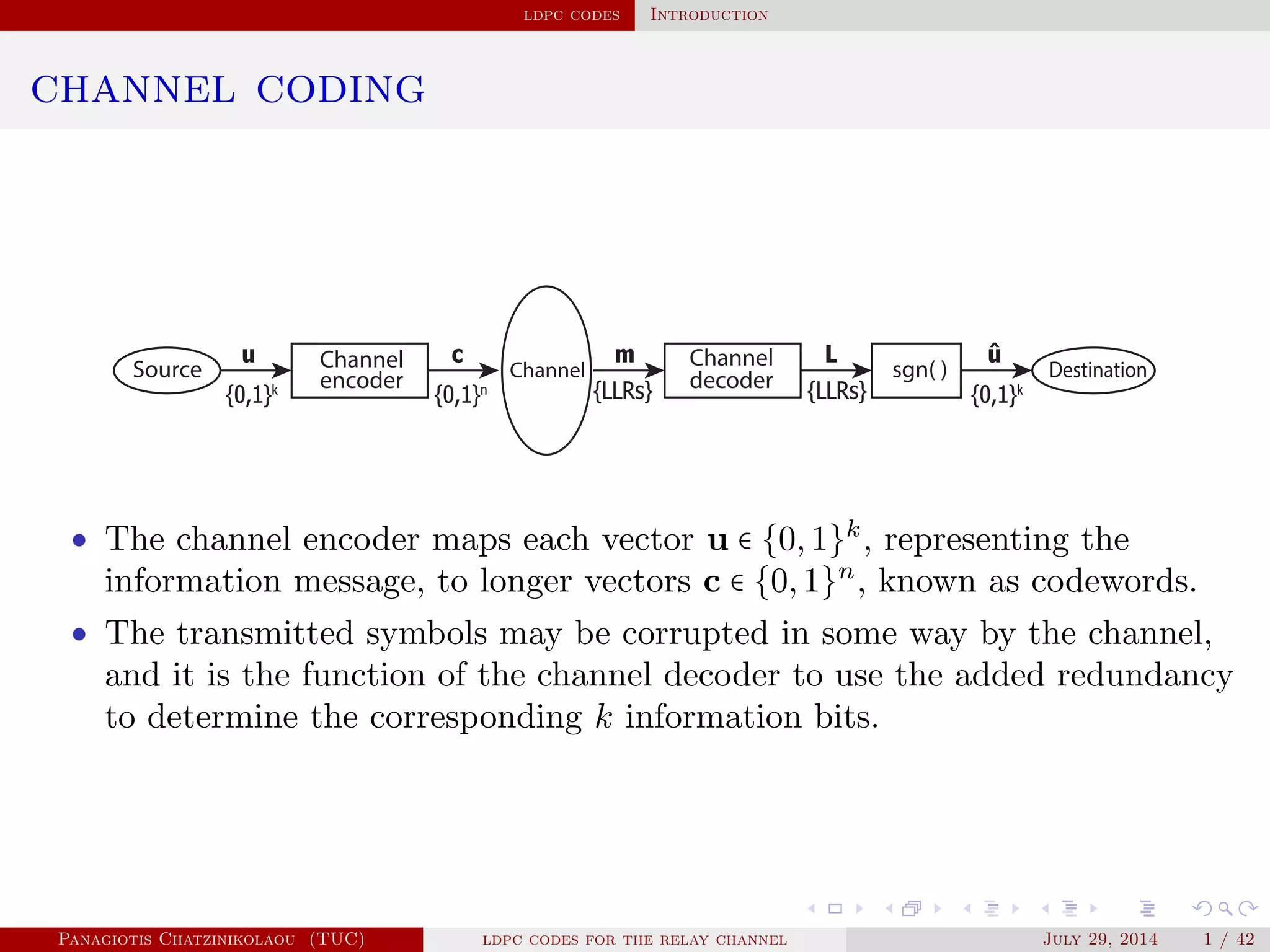
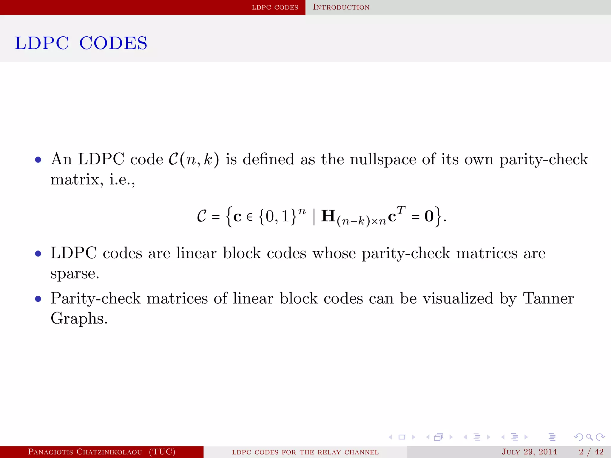
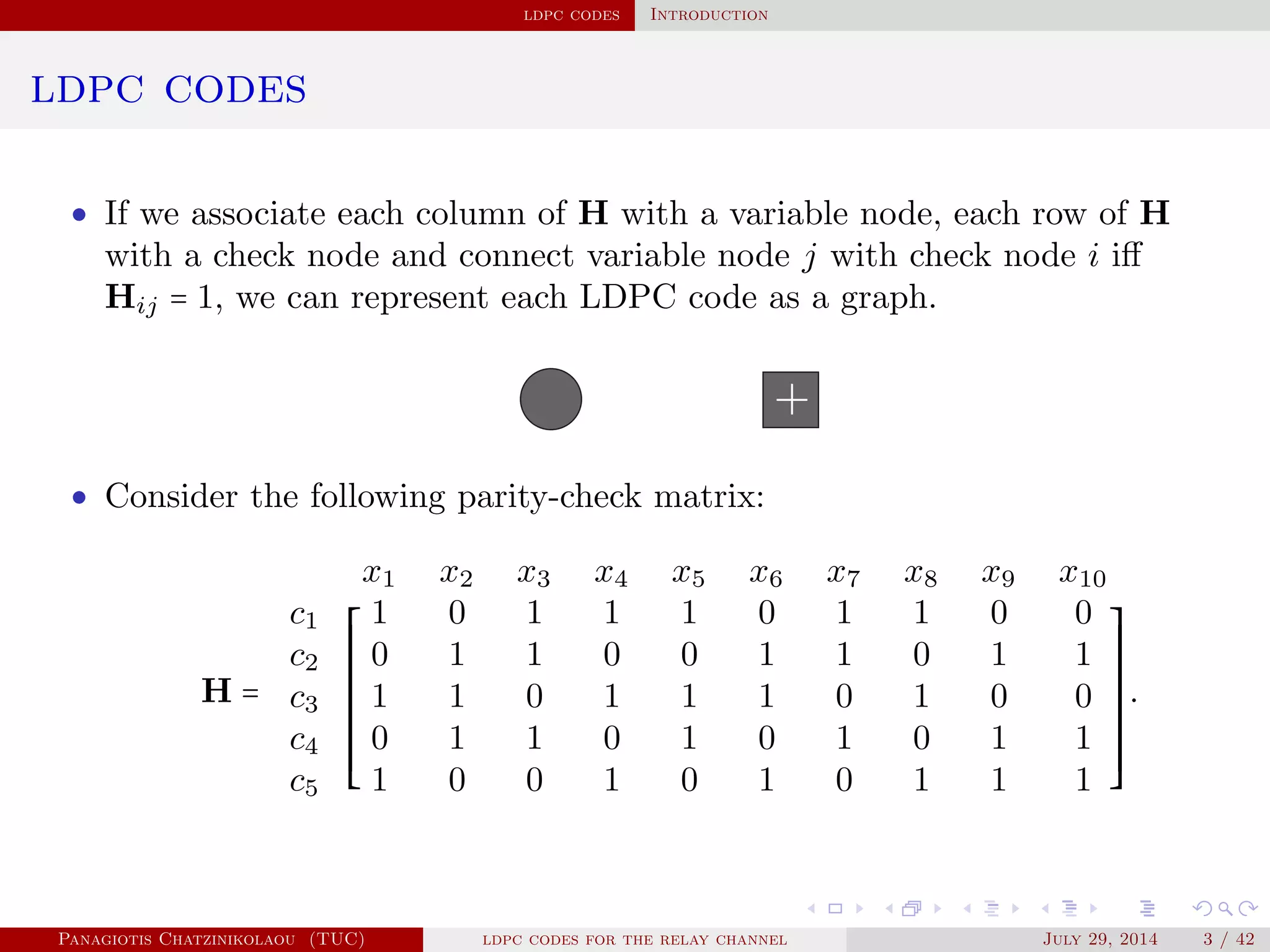
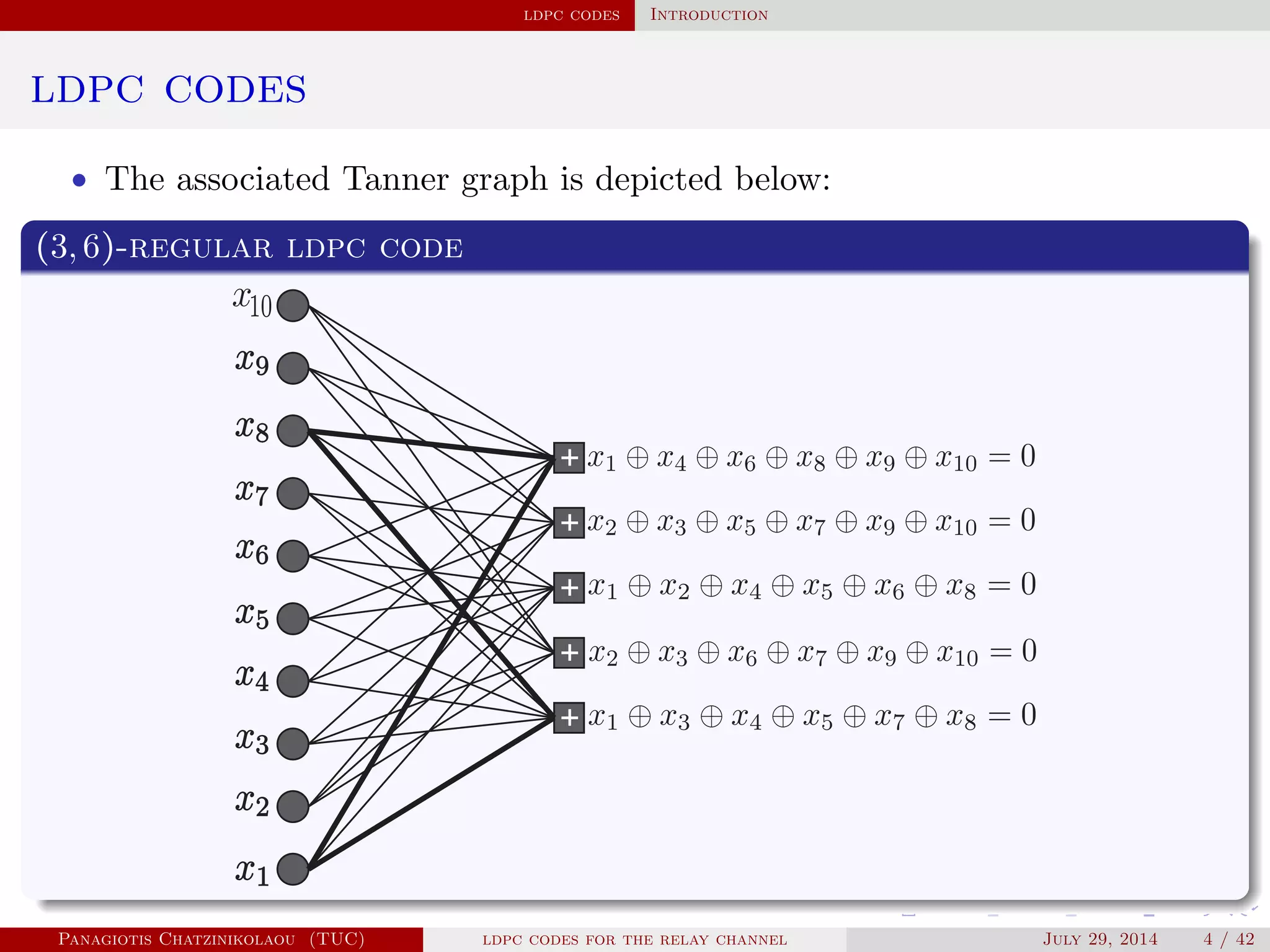
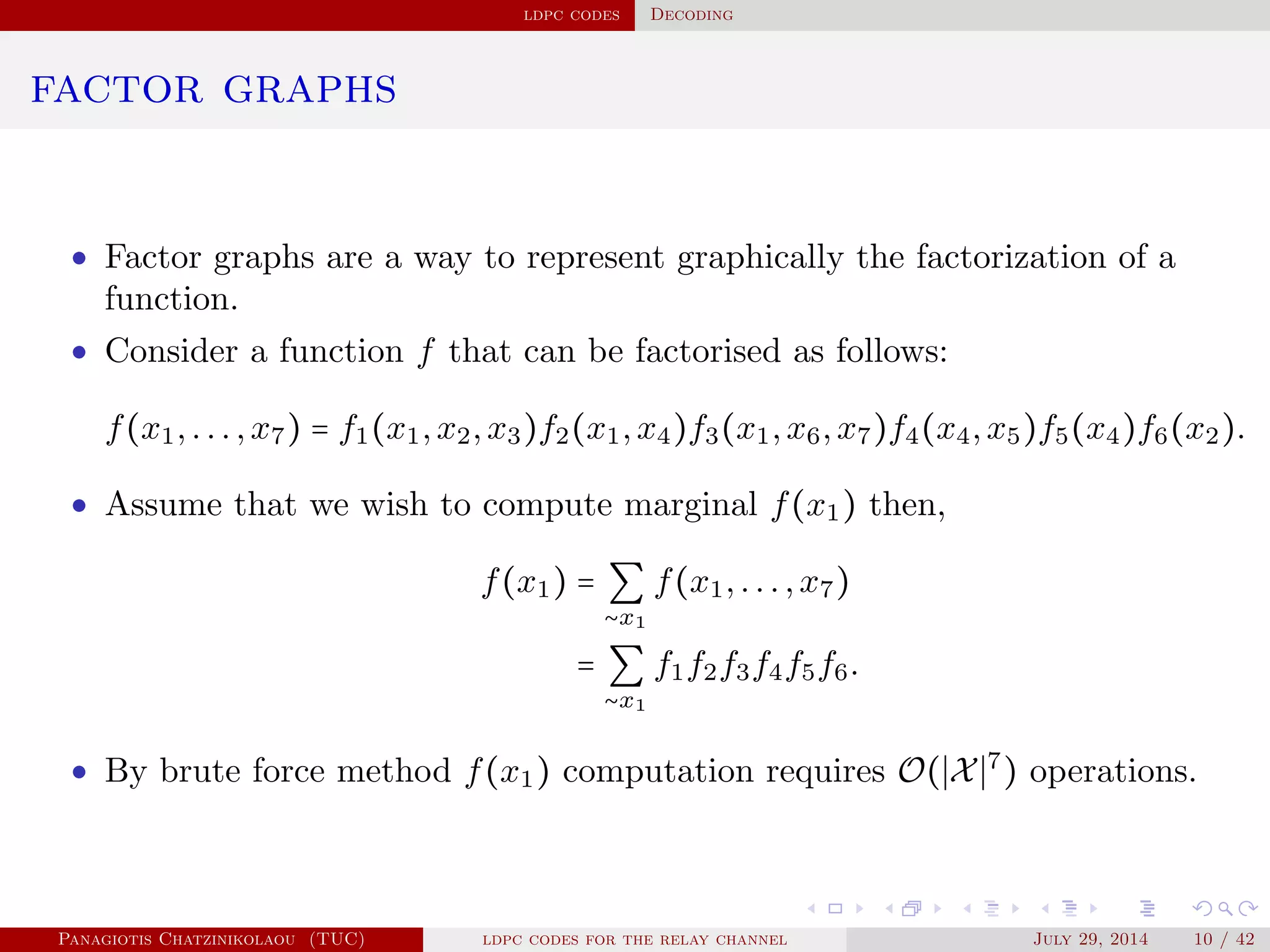
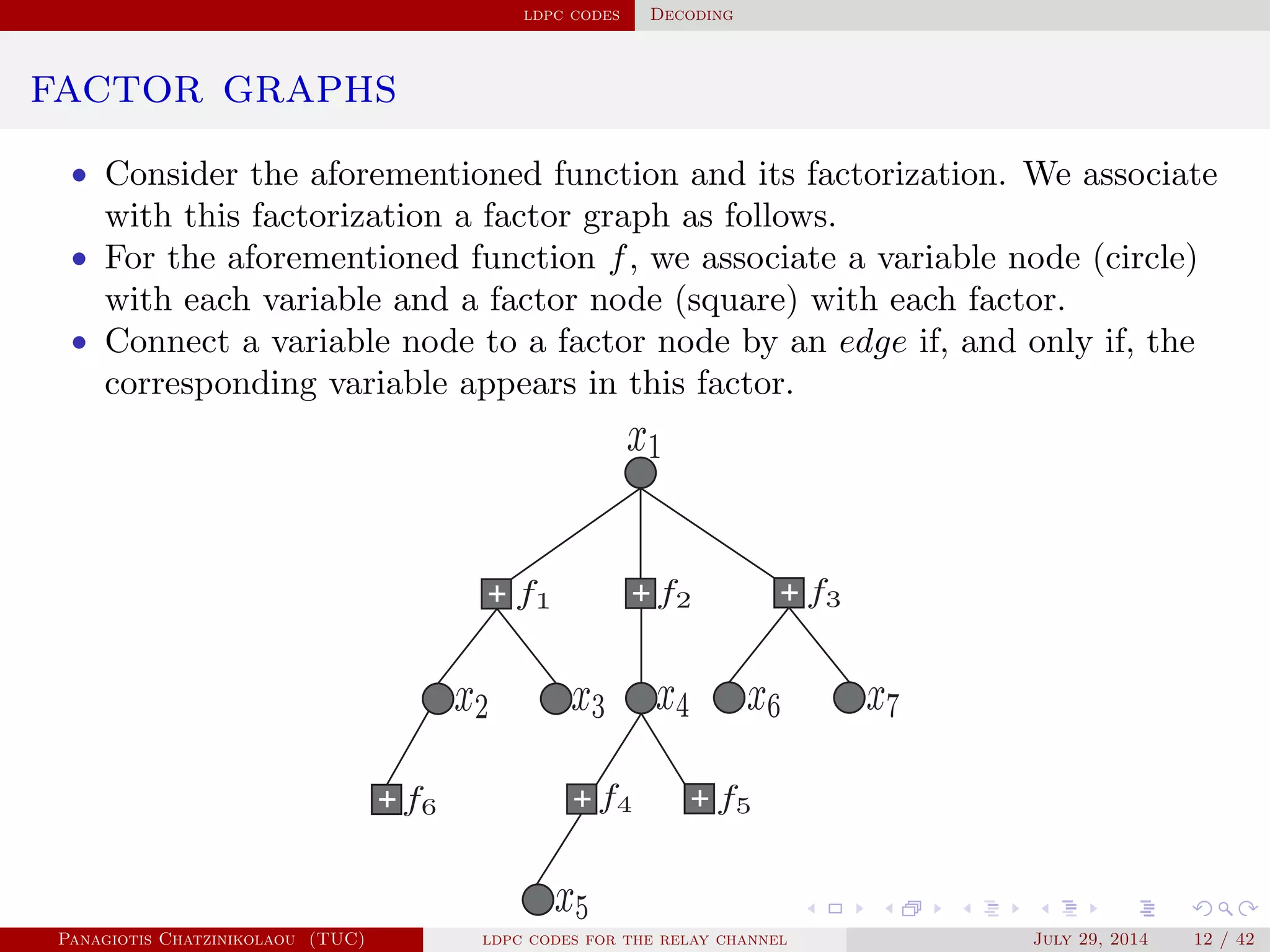
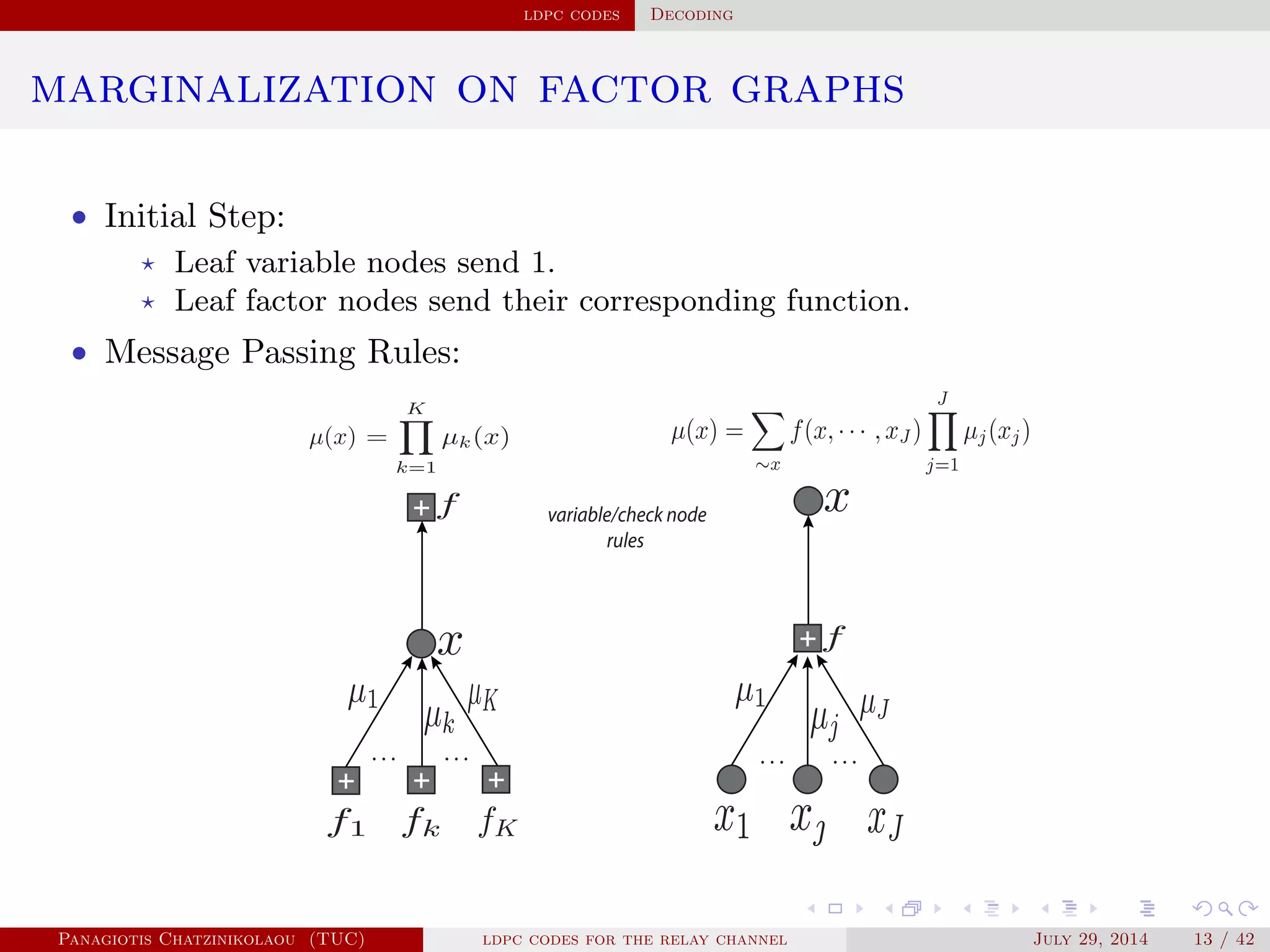
This document discusses low-density parity-check (LDPC) codes and their decoding using belief propagation on factor graphs. It introduces LDPC codes and their representation by sparse parity-check matrices and Tanner graphs. It describes irregular and regular LDPC codes, degree distributions, code ensembles, and decoding using belief propagation on factor graphs and the sum-product algorithm. Examples of decoding a LDPC code over a binary-input additive white Gaussian noise channel are also presented.

![ldpc codes Decoding
factor graphs
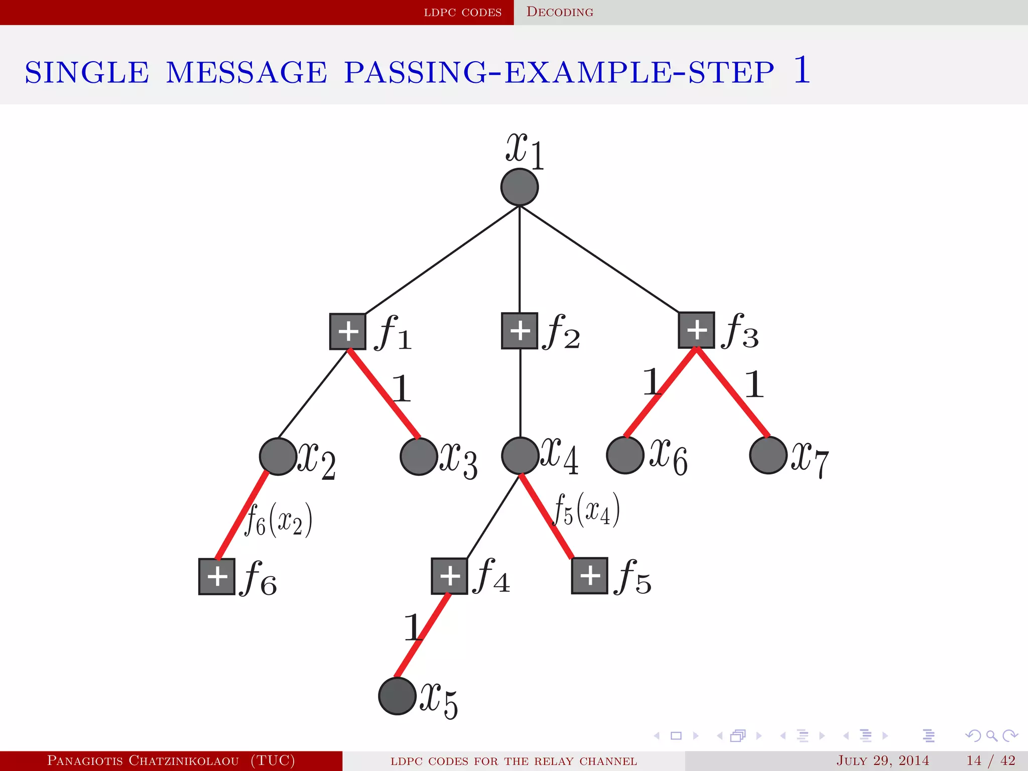
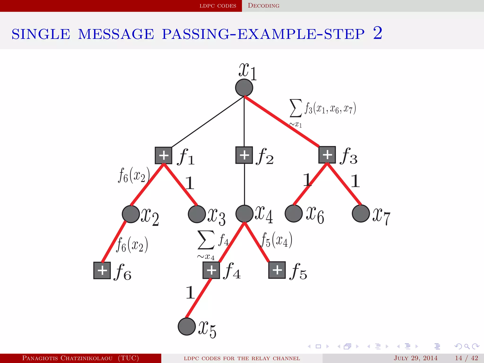
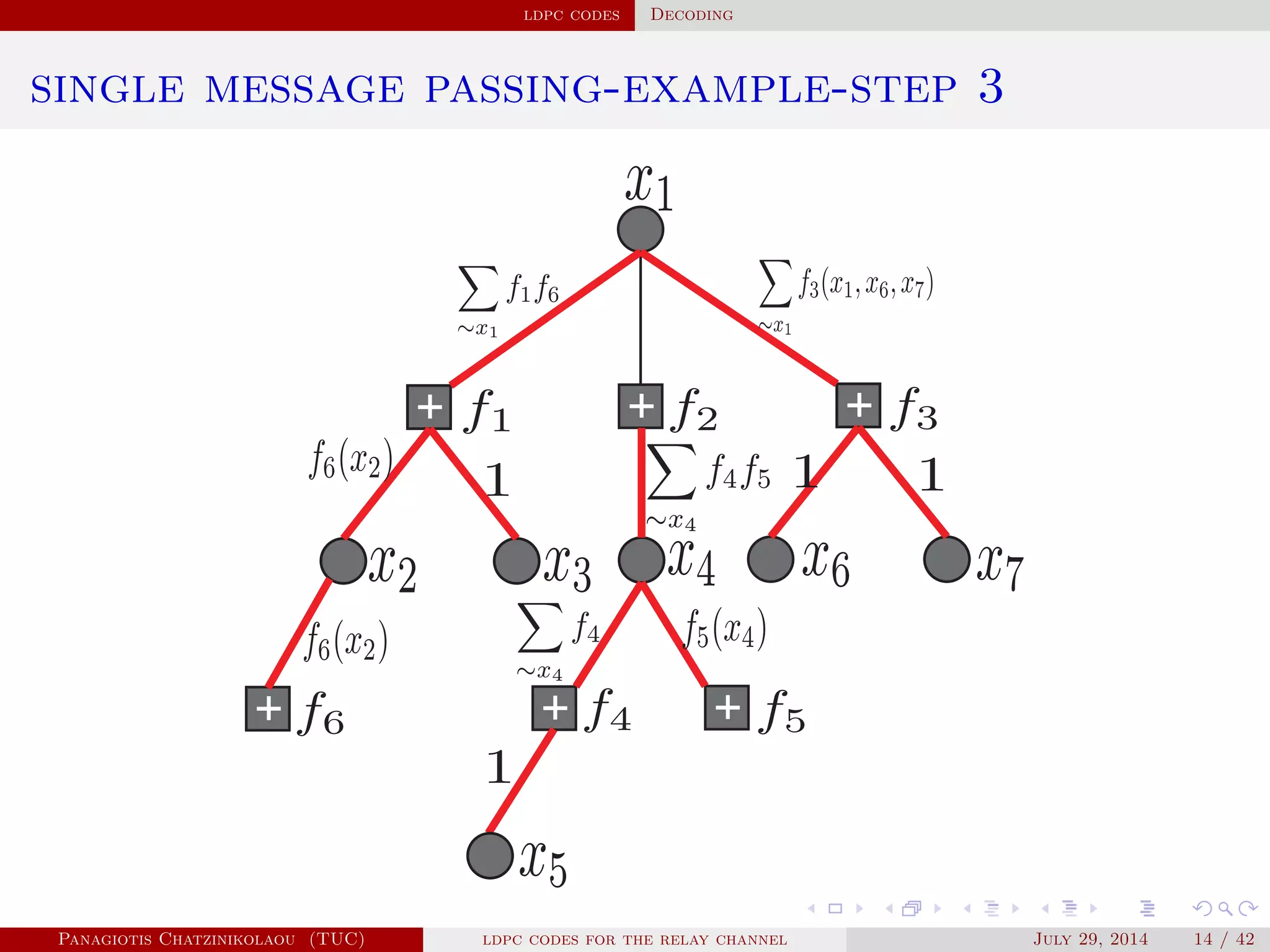
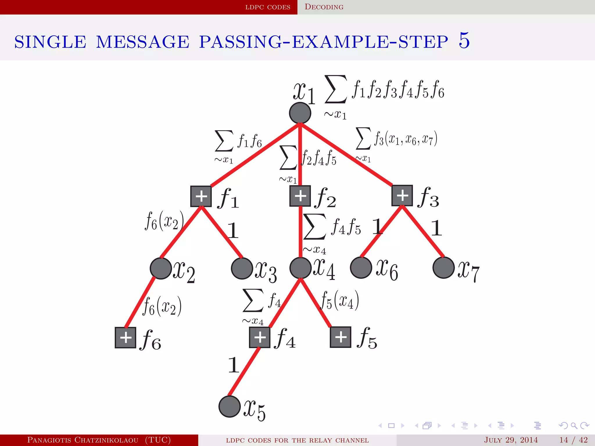
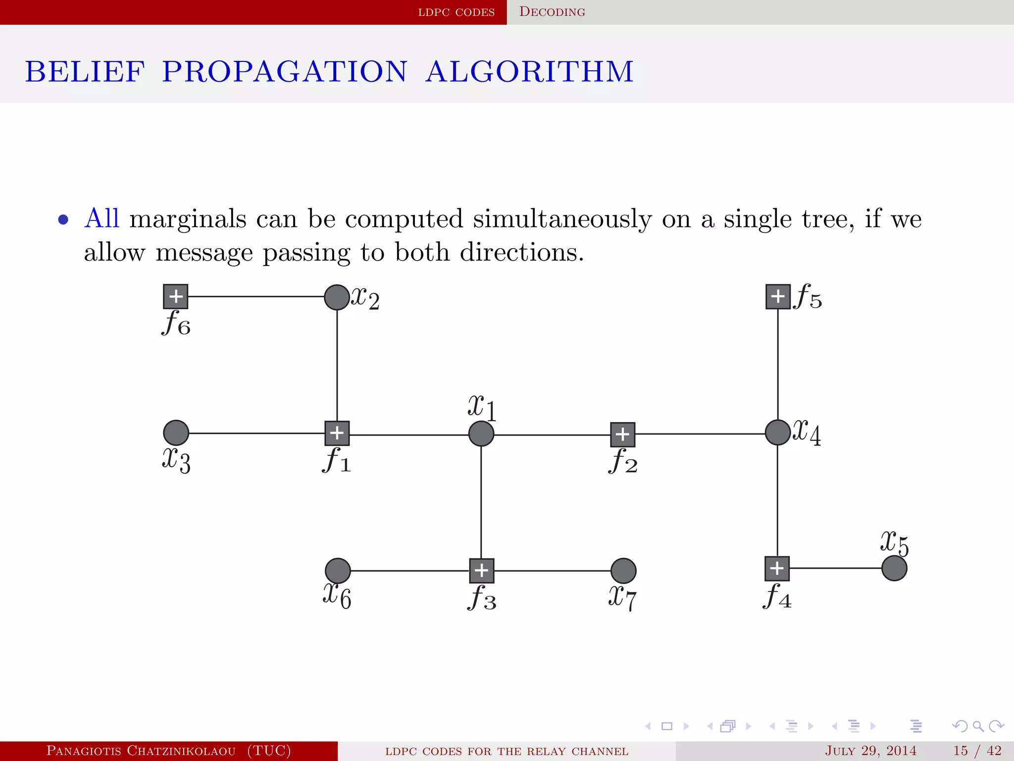
• Applying the factorisation and the distributive law we get
f(x1) = ∑
x2,...,x7
f1(x1,x2,x3)f2(x1,x4)f3(x1,x6,x7)f4(x4,x5)f5(x4)f6(x2)
= [∑
x2
(f6(x2)∑
x3
f1(x1,x2,x3))][∑
x4
(f5(x4)f2(x1,x4)
∑
x5
f4(x4,x5))][ ∑
x6,x7
f3(x1,x6,x7)],
reducing complexity to O( X 3
) !
• Likewise for f(xi), i = 2,...,7.
Panagiotis Chatzinikolaou (TUC) ldpc codes for the relay channel July 29, 2014 11 / 42](https://image.slidesharecdn.com/de0af3e9-e74b-41cb-b01a-28da253839d0-160416144813/75/Thesis_Presentation-13-2048.jpg)


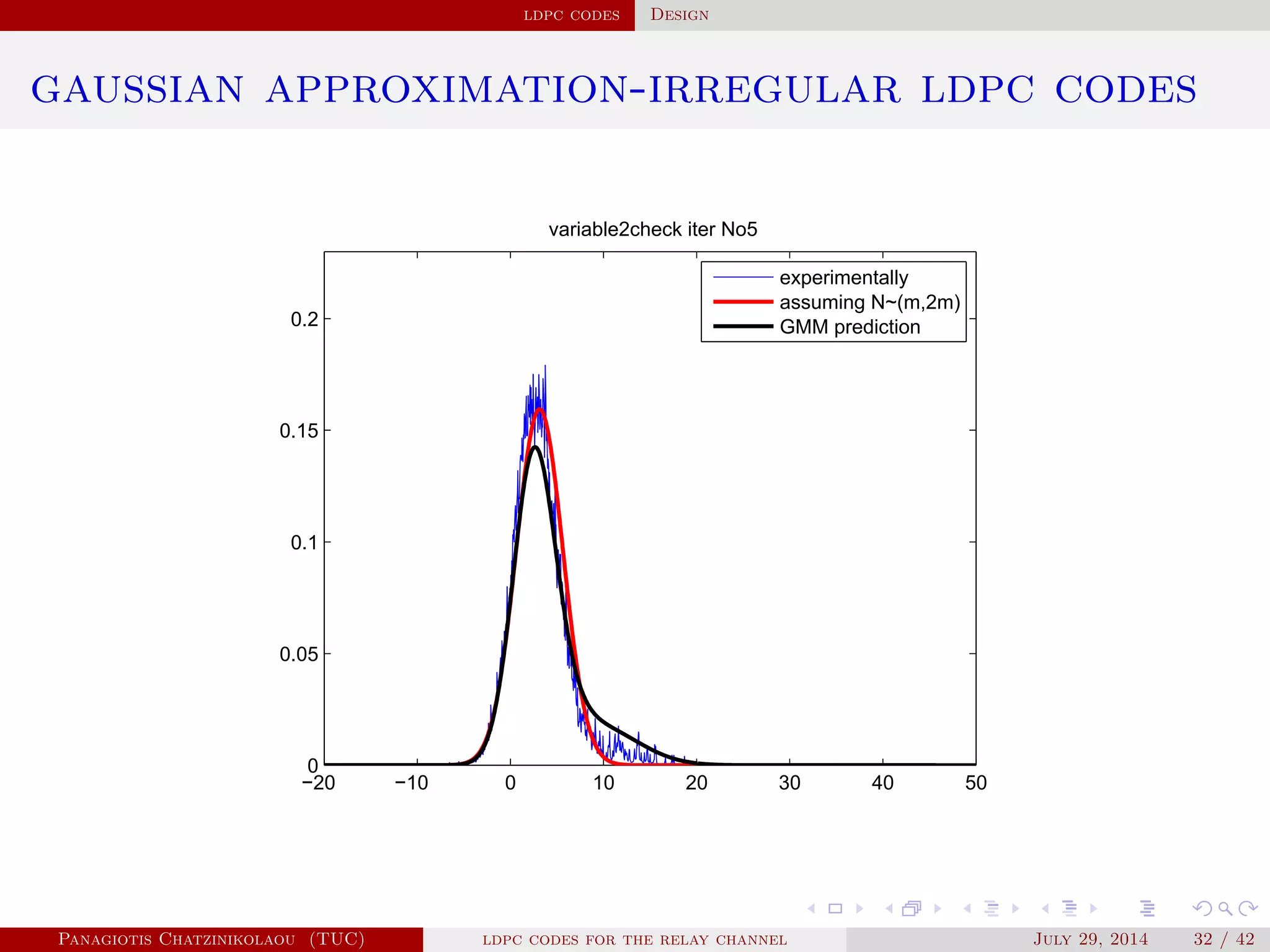
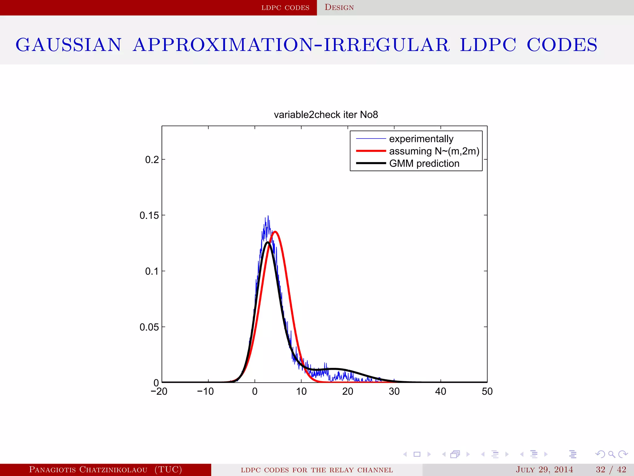
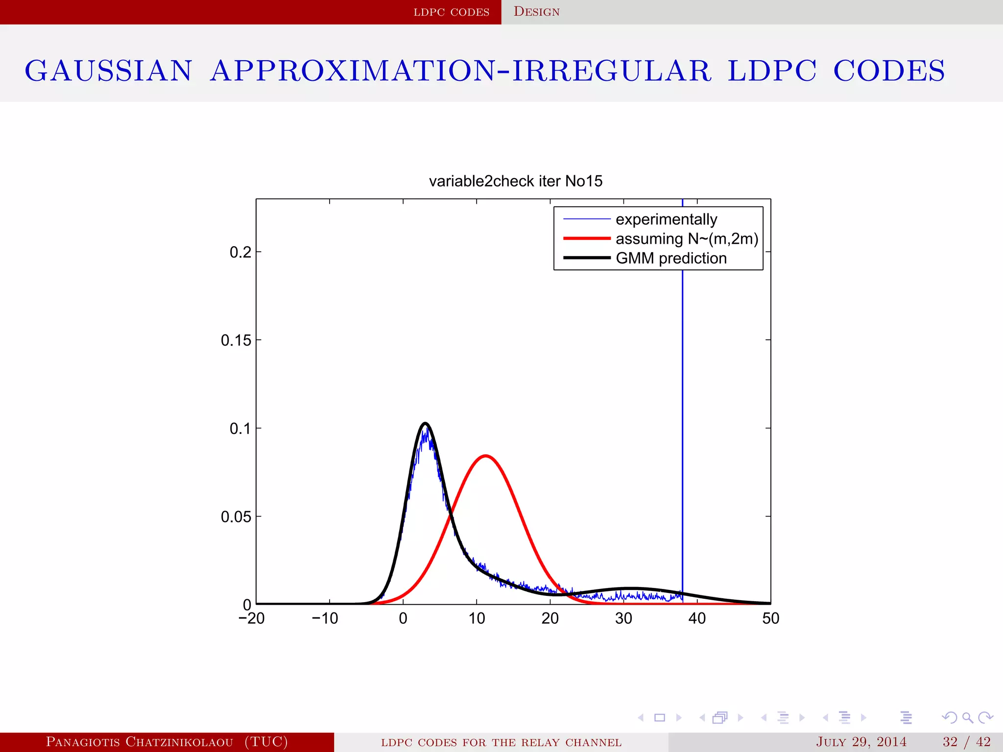
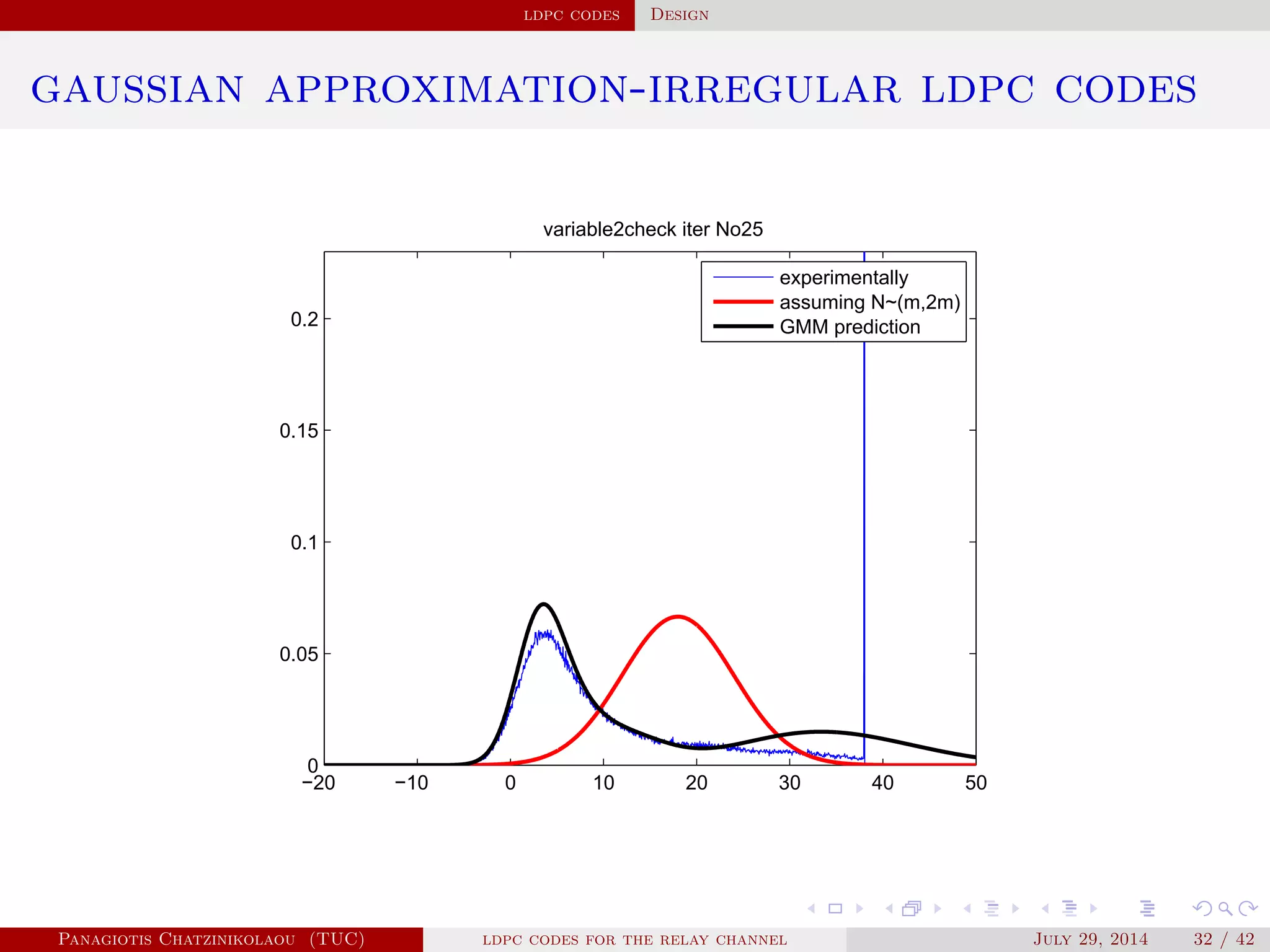
![ldpc codes Design
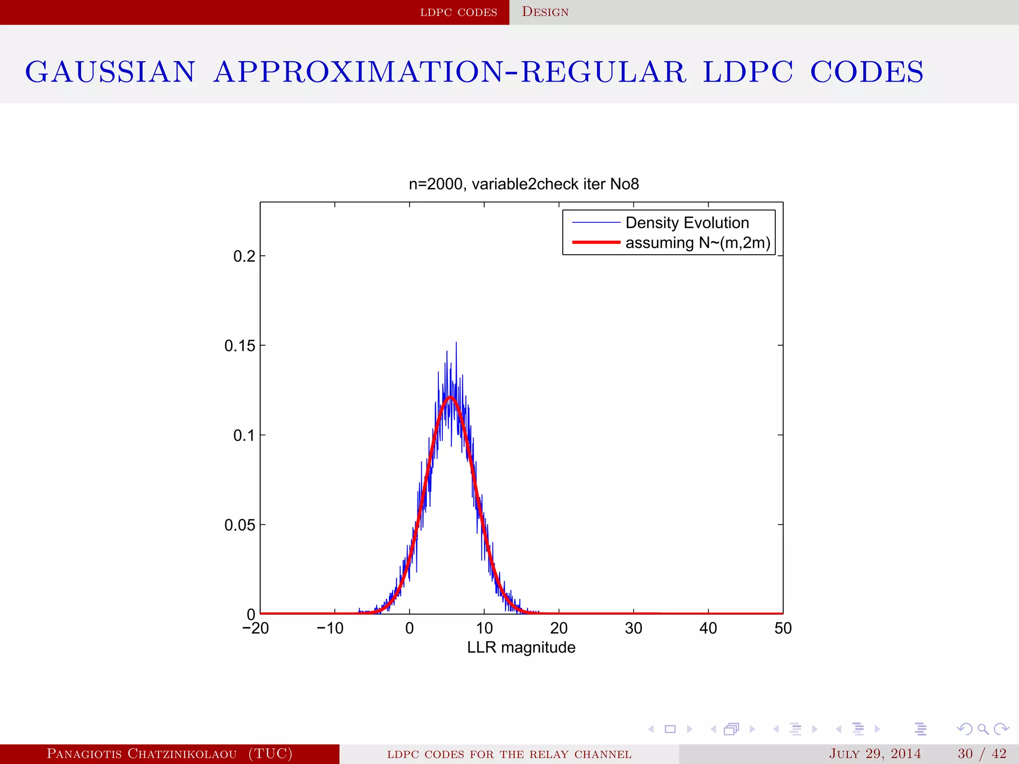
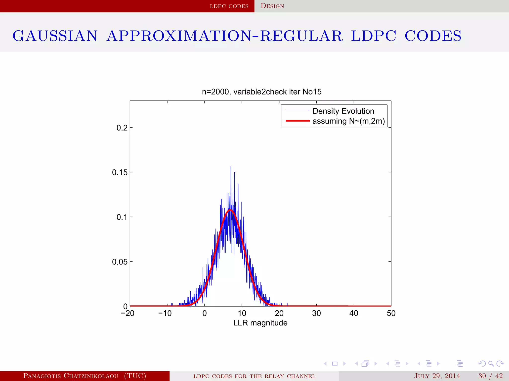
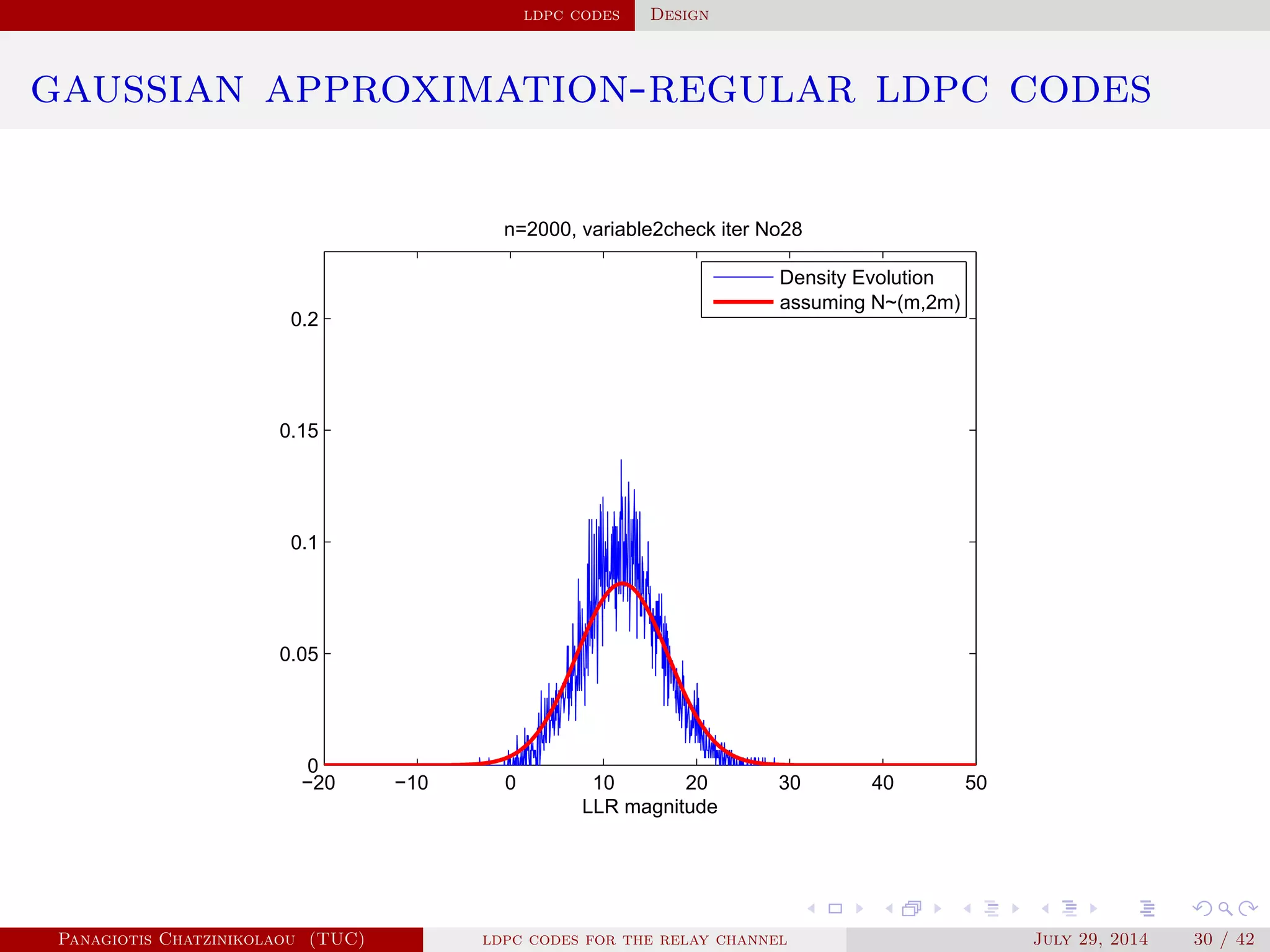
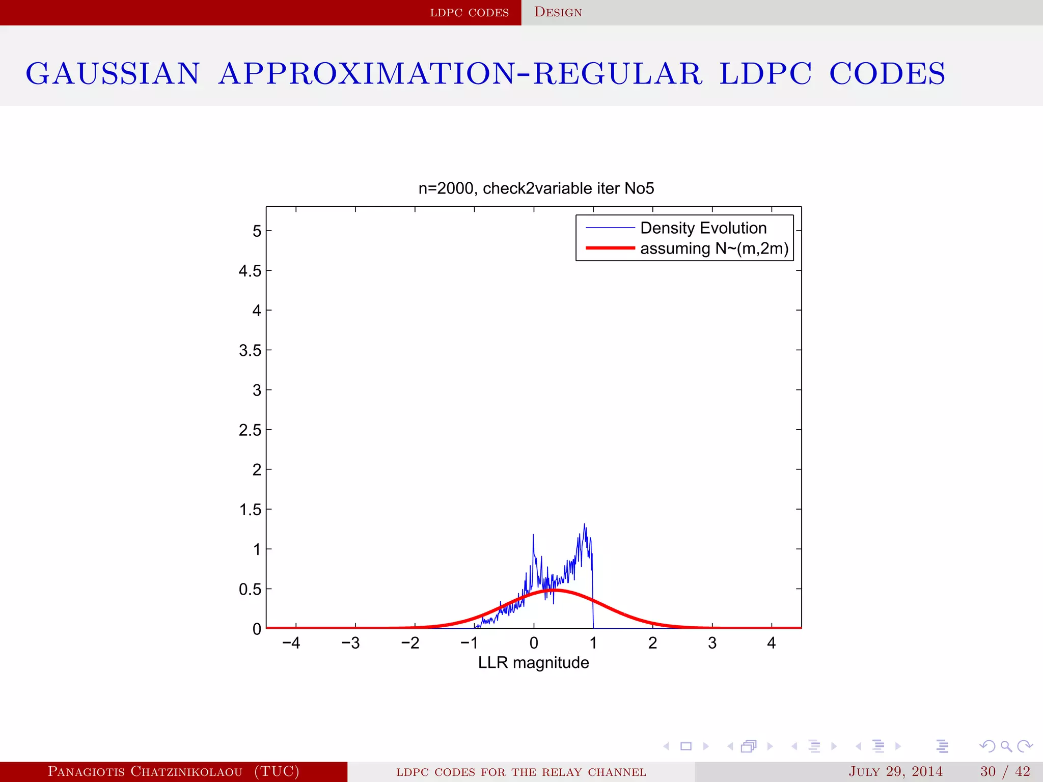
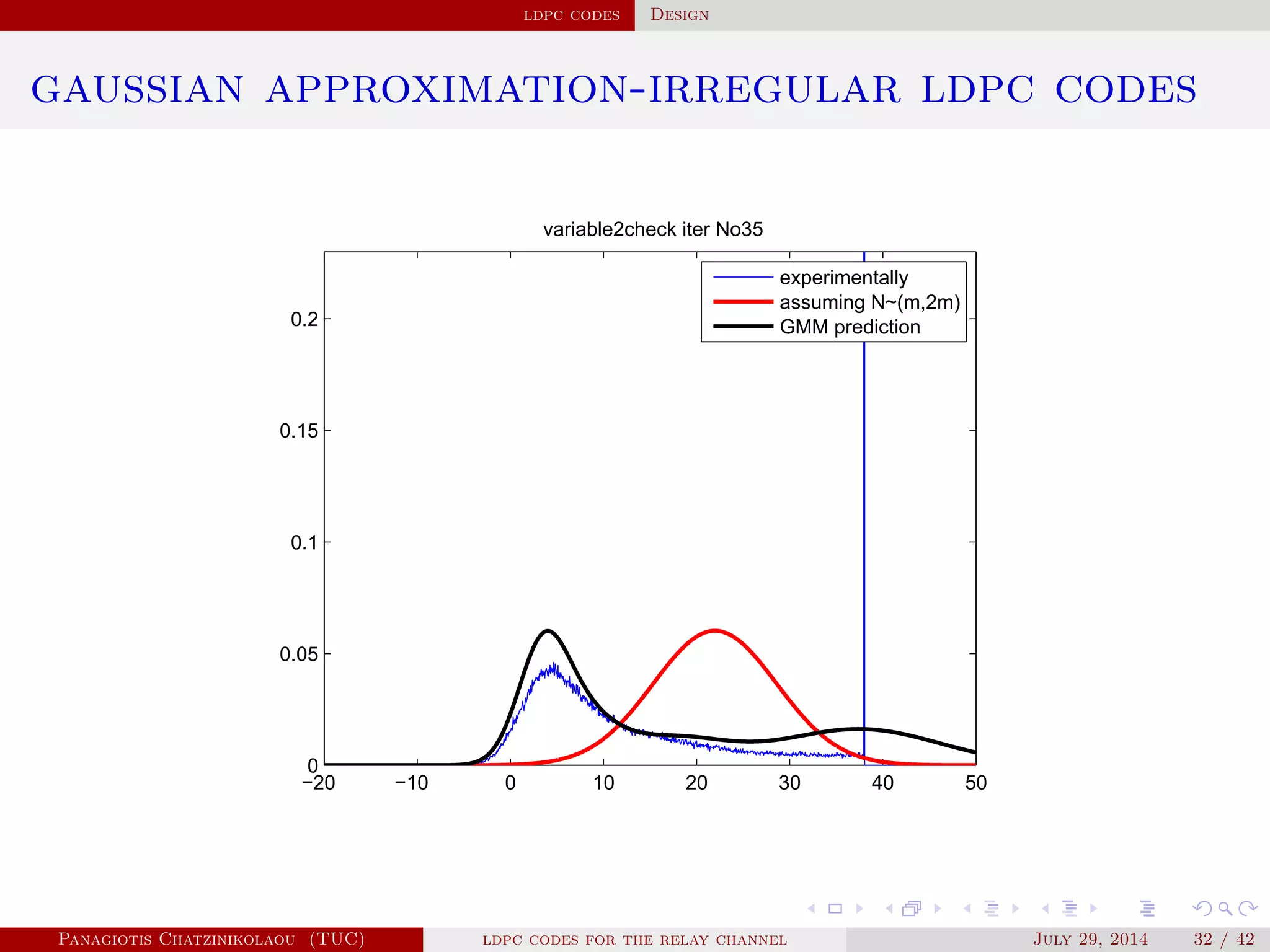
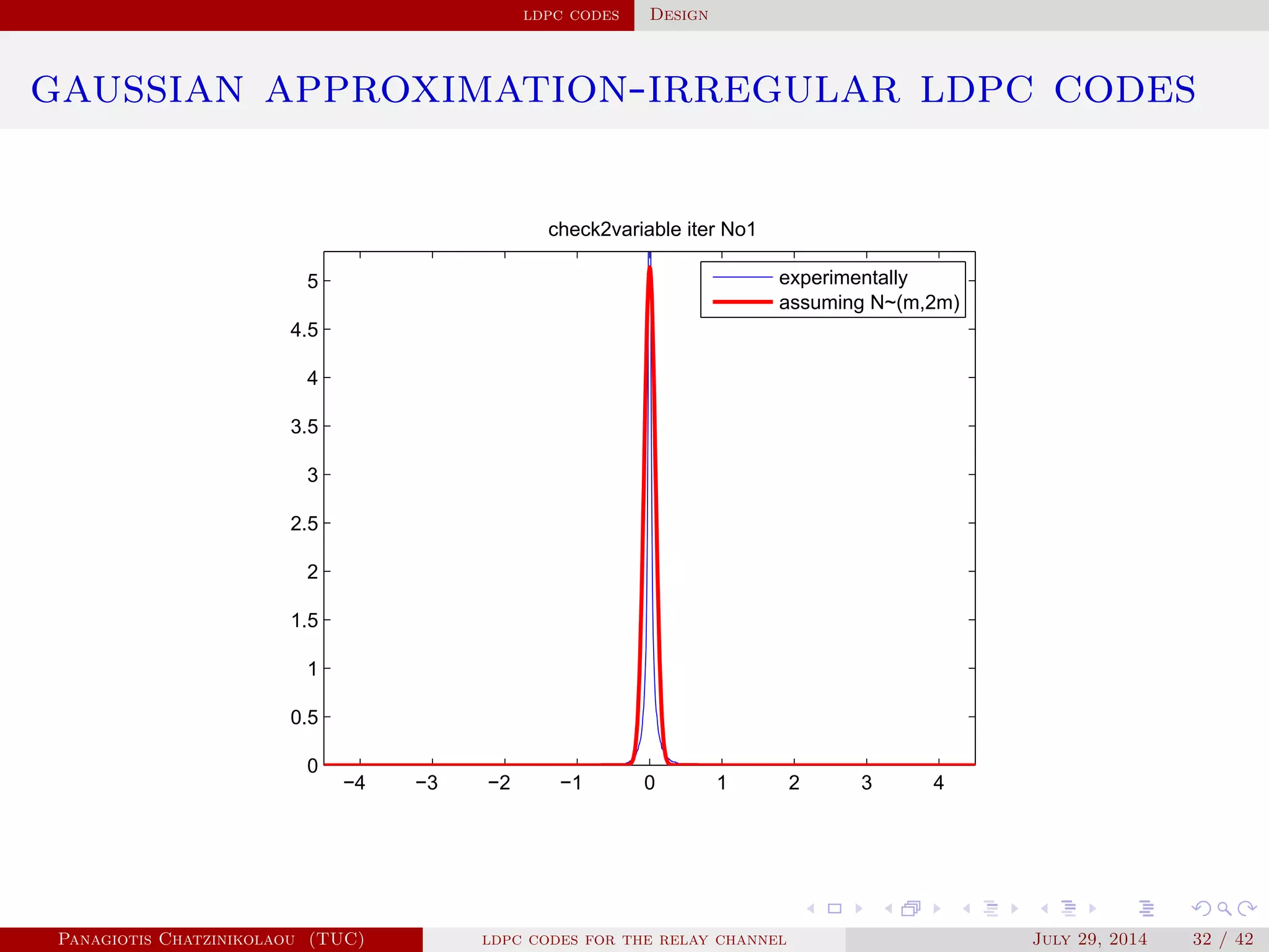
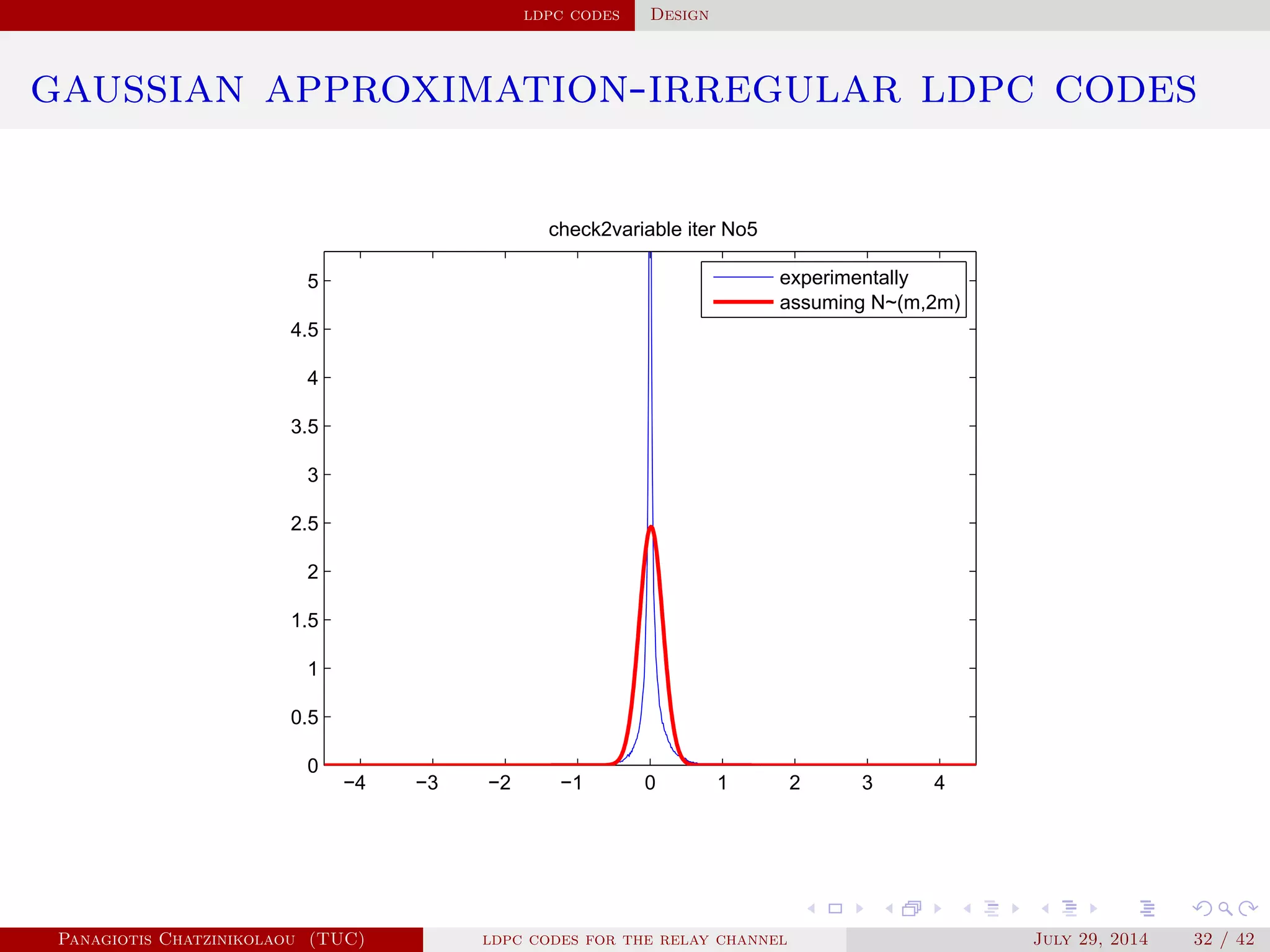
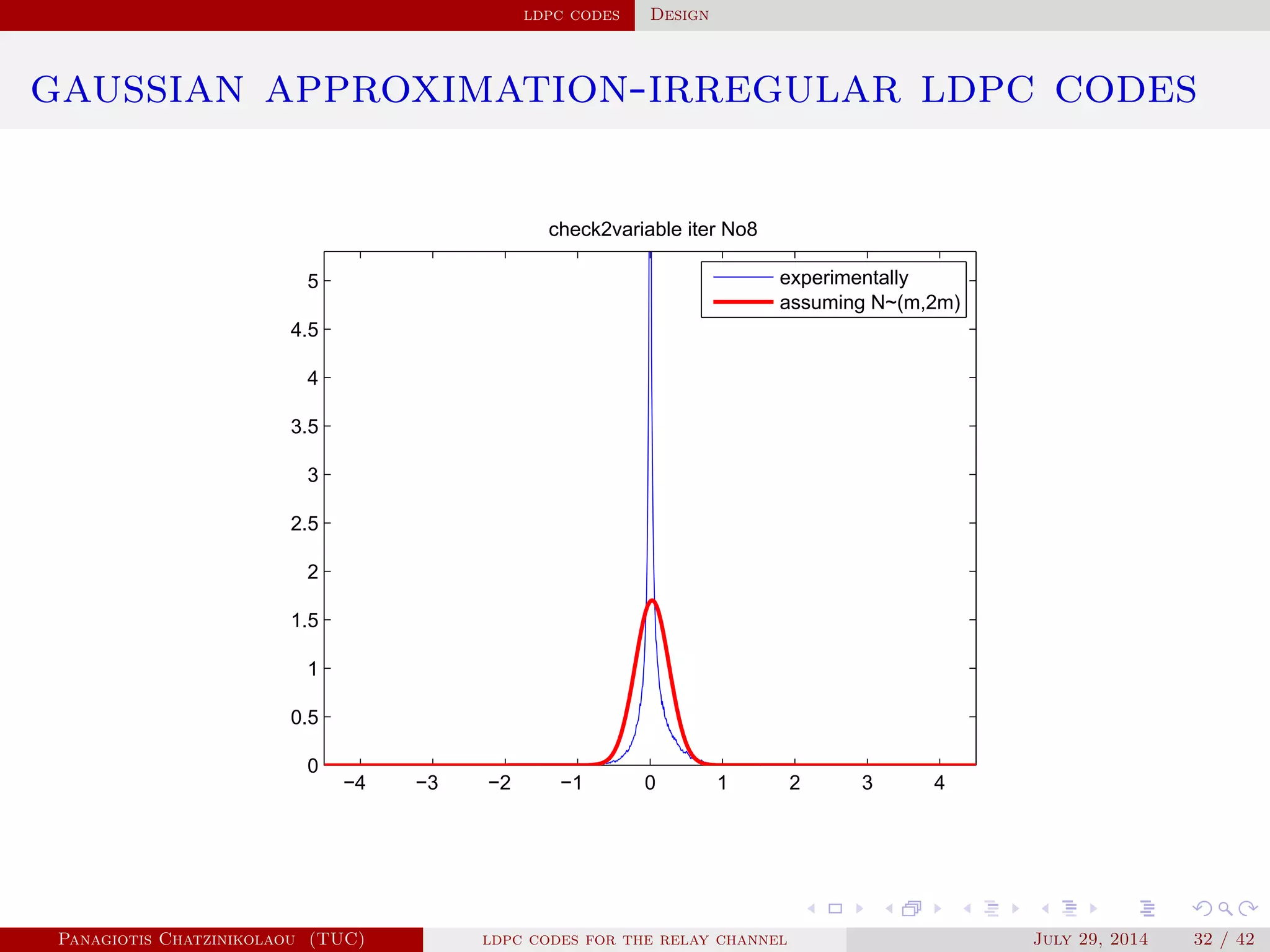
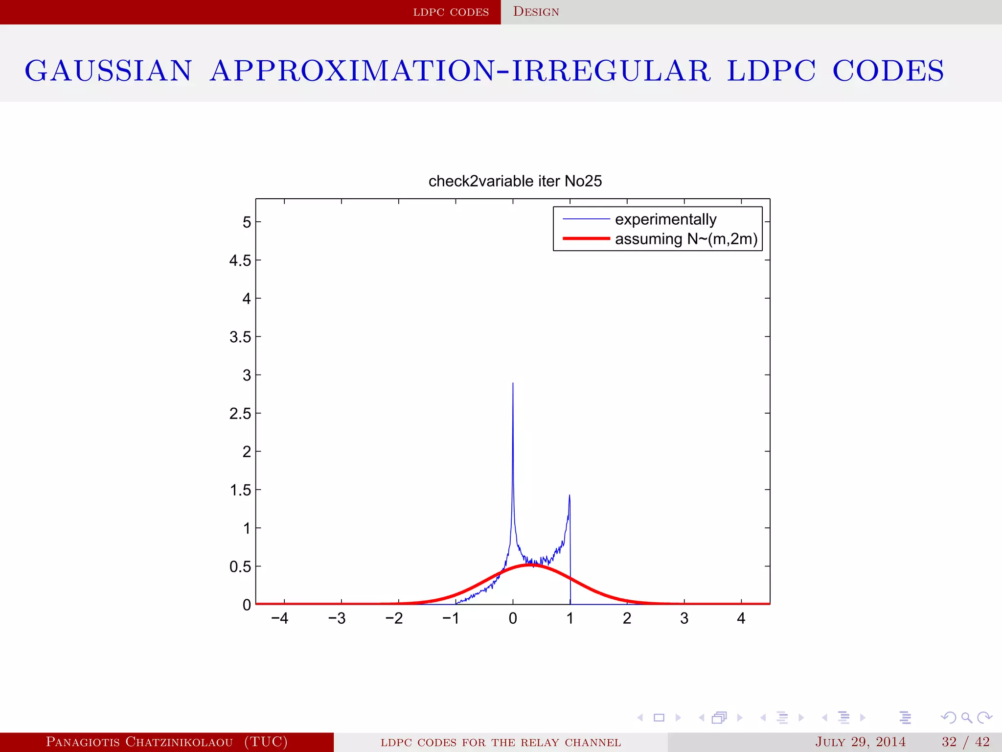
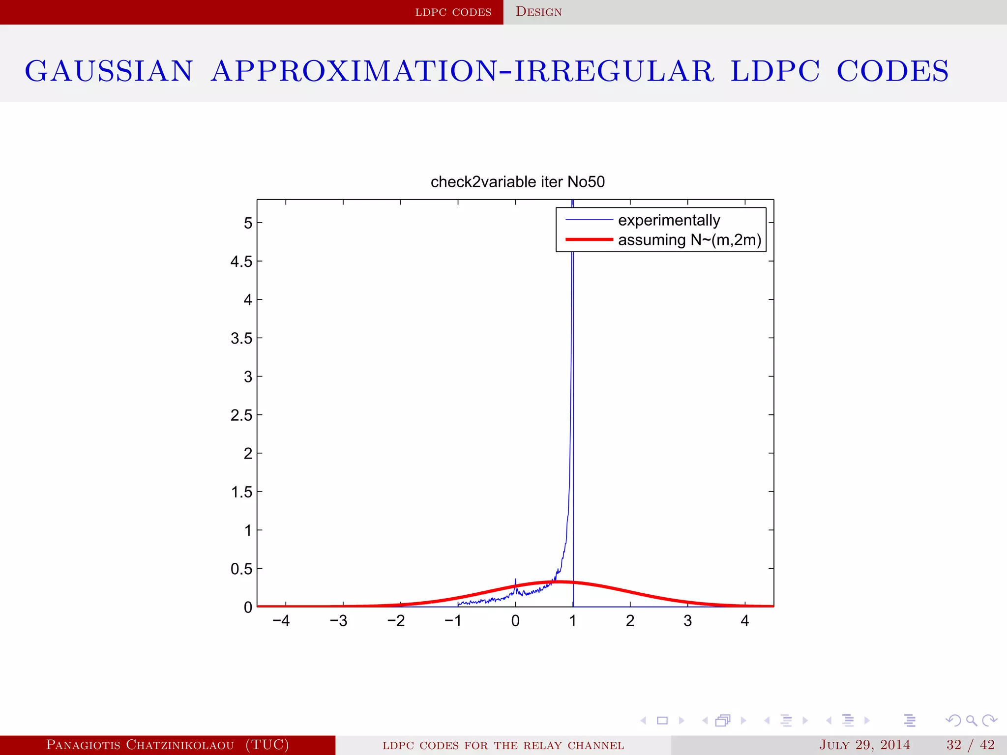
gaussian approximation
• At a variable node of degree i:
µ
( )
v,i = µu0 + (i − 1)µ( −1)
u .
• Averaging over λ(x):
µ( )
v = ∑
i≥2
λiµ
( )
v,i .
• At a check node of degree j:
µ
( )
u,j = φ−1⎛
⎝
1 − [1 − φ(µ( )
v )]
j−1⎞
⎠
.
• Averaging over ρ(x):
µ( )
u = ∑
j≥2
ρjµ
( )
u,j.
Panagiotis Chatzinikolaou (TUC) ldpc codes for the relay channel July 29, 2014 29 / 42](https://image.slidesharecdn.com/de0af3e9-e74b-41cb-b01a-28da253839d0-160416144813/75/Thesis_Presentation-45-2048.jpg)


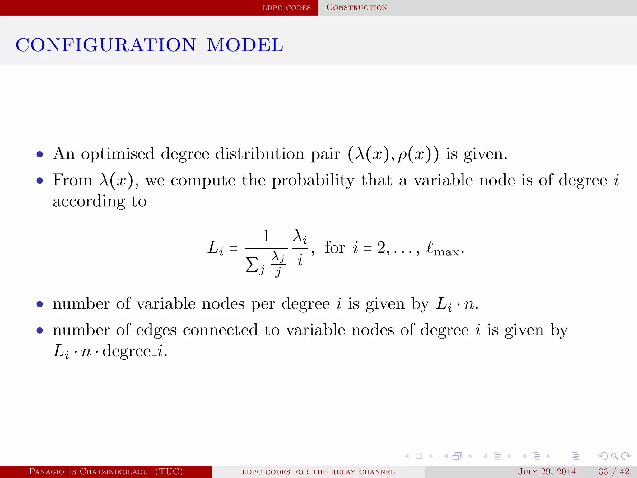
![ldpc codes Construction
configuration model
• “Generate” n variable nodes and m check nodes with their sockets.
• Label the variable and check node sockets separately with the set
[Λ′
(1)] = {1,...,∑i iΛi}.
.
.
.
.
.
.
v1
v2
vn
C2
C1
C m
v3
C3
1
2
3
4
5
6
7
1
2
.
.
.
total_edges
total_edges
.
.
.
.
.
.
total edges is the last socket (edge) which is equal to the total number of
edges (= ∑i iΛi).
Panagiotis Chatzinikolaou (TUC) ldpc codes for the relay channel July 29, 2014 33 / 42](https://image.slidesharecdn.com/de0af3e9-e74b-41cb-b01a-28da253839d0-160416144813/75/Thesis_Presentation-92-2048.jpg)
![ldpc codes Construction
configuration model
• Pick a permutation π on [Λ′
(1)] at random with uniform probability
from the set of all (∑i iΛi)! such permutations.
• Let π be a permutation on [Λ′
(1)]. Connect i-th variable node edge
socket with π(i)-th check node edge socket.
.
.
.
.
.
.
v1
v2
vn
C2
C1
C m
v3
C3
1
2
3
4
5
6
7
total_edges
.
.
.
π(1)
π(2)
π(3)
• Put “1” in the appropriate position of H.
Panagiotis Chatzinikolaou (TUC) ldpc codes for the relay channel July 29, 2014 33 / 42](https://image.slidesharecdn.com/de0af3e9-e74b-41cb-b01a-28da253839d0-160416144813/75/Thesis_Presentation-93-2048.jpg)
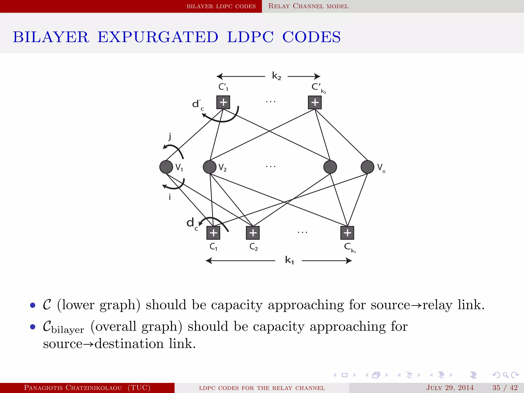
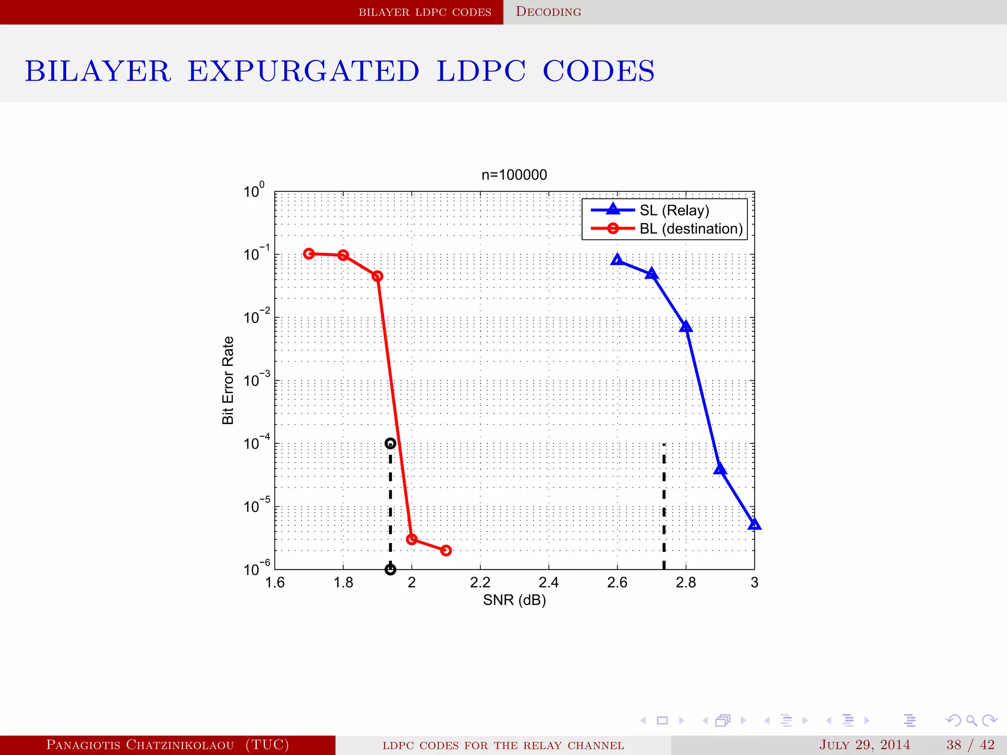
![bilayer ldpc codes Relay Channel model
relay channel
1 For the source-relay link, x ∈ C, with parity-check matrix H such that
Hx = 0.
2 rate(C) ≤ rate(source → relay). Hence, relay decodes x.
3 rate(C) > rate(source → destination). Hence, destination cannot decode x.
4 The parity-check matrix of Cbilayer denoted by Hbilayer is given by
Hbilayer = [
H
H1
], Hbilayer ⋅ x = [
0
p
],
where H1 is the upper layer of the bilayer graph.
5 Finally, rate(Cbilayer) ≤ rate(source → destination) and, therefore,
destination decodes x using Hbilayer and parity vector p sent by the relay.
Panagiotis Chatzinikolaou (TUC) ldpc codes for the relay channel July 29, 2014 34 / 42](https://image.slidesharecdn.com/de0af3e9-e74b-41cb-b01a-28da253839d0-160416144813/75/Thesis_Presentation-94-2048.jpg)
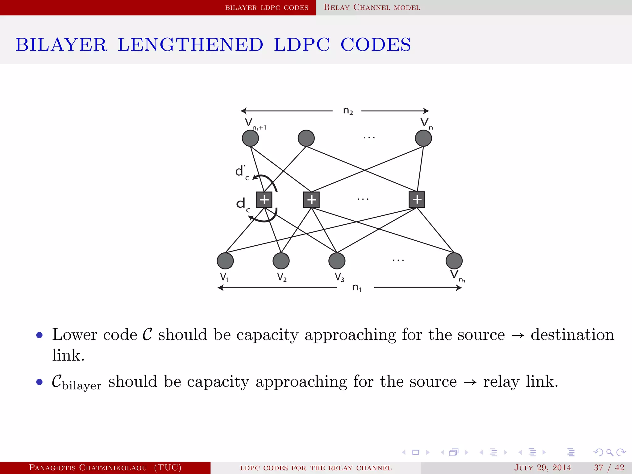
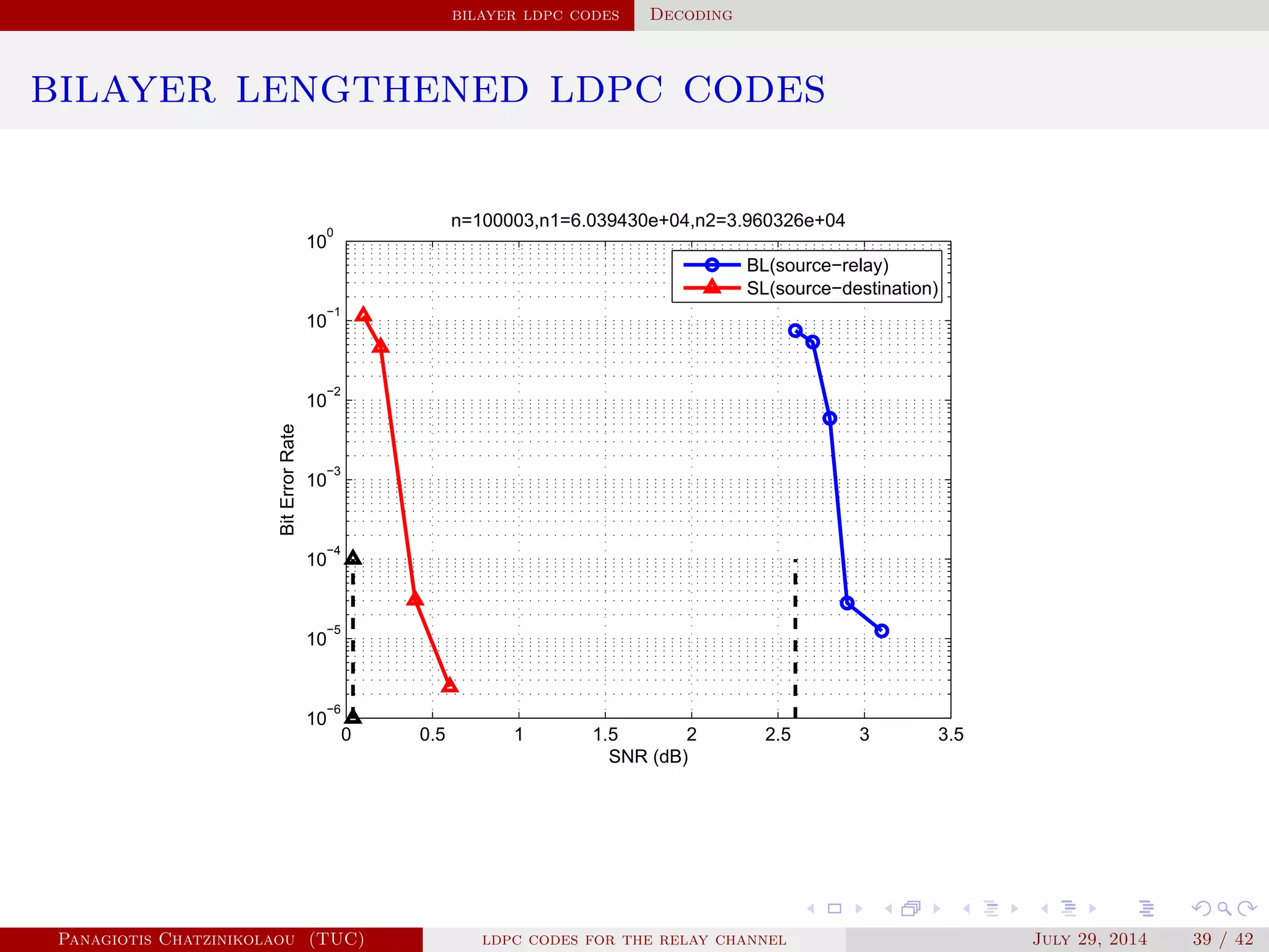
![bilayer ldpc codes Relay Channel model
bilayer lengthened ldpc codes
1 For the source-relay link, x ∈ Cbilayer, with parity-check matrix Hbilayer
such that Hbilayerx = 0.
2 rate(C) ≤ rate(source → relay). Hence, relay decodes x over the bilayer
graph.
3 rate(C) > rate(source → destination). Hence, destination cannot decode x.
4 The parity-check matrix of Cbilayer denoted by Hbilayer is given by
Hbilayer = [H H1],
where H1 is the upper layer of the bilayer graph.
5 The relay forwards to the destination the upper n2 variable nodes.
Destination removes the upper variable nodes, reducing the resulting
code’s rate and decodes the lower graph.
Panagiotis Chatzinikolaou (TUC) ldpc codes for the relay channel July 29, 2014 36 / 42](https://image.slidesharecdn.com/de0af3e9-e74b-41cb-b01a-28da253839d0-160416144813/75/Thesis_Presentation-96-2048.jpg)


![RF Circuit Design - [Ch3-1] Microwave Network](https://cdn.slidesharecdn.com/ss_thumbnails/ch3-1-150613064402-lva1-app6892-thumbnail.jpg?width=640&height=640&fit=bounds)


![RF Circuit Design - [Ch2-1] Resonator and Impedance Matching](https://cdn.slidesharecdn.com/ss_thumbnails/ch2-1-150613064353-lva1-app6892-thumbnail.jpg?width=640&height=640&fit=bounds)