the population ecology 53_lecture_presentation_0.ppt

Copyright © 2008 Pearson Education, Inc., publishing as Pearson Benjamin Cummings
PowerPoint®
Lecture Presentations for
Biology
Eighth Edition
Neil Campbell and Jane Reece
Lectures by Chris Romero, updated by Erin Barley with contributions from Joan Sharp
Chapter 53
Population Ecology

Overview
• Population ecology is the study of
populations in relation to environment,
including environmental influences on density
and distribution, age structure, and population
size.
• A population is a group of individuals of a
single species living in the same general area.

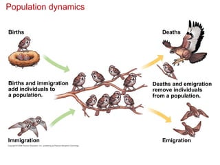
Dynamic biological processes influence population
density, dispersion, and demographics
• Density is the number of individuals per unit
area or volume.
• Dispersion is the pattern of spacing among
individuals within the boundaries of the
population.
• Density is the result of an interplay between
processes that add individuals to a population
and those that remove individuals.

• Immigration is the influx of new individuals from other
areas.
• Emigration is the movement of individuals out of a
population.
• In most cases, it is impractical or impossible to count
all individuals in a population. Sampling techniques
can be used to estimate densities and total population
sizes.
• Population size can be estimated by either
extrapolation from small samples, an index of
population size, or the Mark-Recapture Method.

Population dynamics
Births
Births and immigration
add individuals to
a population.
Immigration
Deaths and emigration
remove individuals
from a population.
Deaths
Emigration

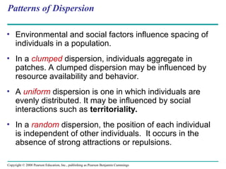
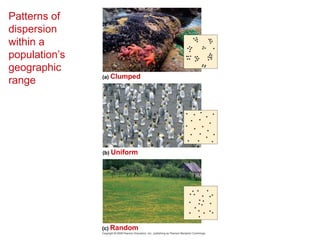
Patterns of Dispersion
• Environmental and social factors influence spacing of
individuals in a population.
• In a clumped dispersion, individuals aggregate in
patches. A clumped dispersion may be influenced by
resource availability and behavior.
• A uniform dispersion is one in which individuals are
evenly distributed. It may be influenced by social
interactions such as territoriality.
• In a random dispersion, the position of each individual
is independent of other individuals. It occurs in the
absence of strong attractions or repulsions.

Patterns of
dispersion
within a
population’s
geographic
range (a) Clumped
(b) Uniform
(c) Random

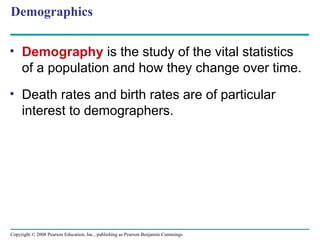
Demographics
• Demography is the study of the vital statistics
of a population and how they change over time.
• Death rates and birth rates are of particular
interest to demographers.

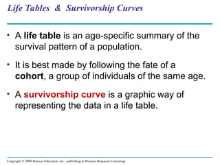
Life Tables & Survivorship Curves
• A life table is an age-specific summary of the
survival pattern of a population.
• It is best made by following the fate of a
cohort, a group of individuals of the same age.
• A survivorship curve is a graphic way of
representing the data in a life table.

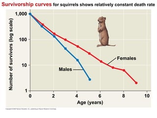
Survivorship curves for squirrels shows relatively constant death rate
Age (years)
2
0 4 8
6
10
10
1
1,000
100
Number
of
survivors
(log
scale)
Males
Females

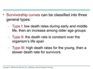
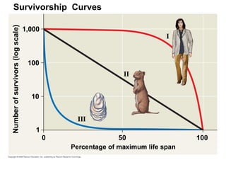
• Survivorship curves can be classified into three
general types:
– Type I: low death rates during early and middle
life, then an increase among older age groups
– Type II: the death rate is constant over the
organism’s life span
– Type III: high death rates for the young, then a
slower death rate for survivors

Survivorship Curves
1,000
100
10
1
0 50 100
II
III
Percentage of maximum life span
Number
of
survivors
(log
scale)
I

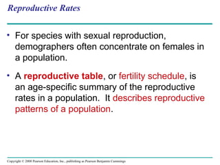
Reproductive Rates
• For species with sexual reproduction,
demographers often concentrate on females in
a population.
• A reproductive table, or fertility schedule, is
an age-specific summary of the reproductive
rates in a population. It describes reproductive
patterns of a population.

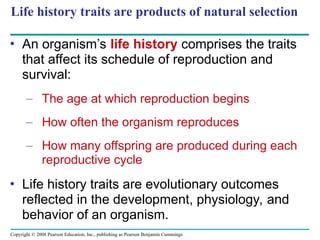
Life history traits are products of natural selection
• An organism’s life history comprises the traits
that affect its schedule of reproduction and
survival:
– The age at which reproduction begins
– How often the organism reproduces
– How many offspring are produced during each
reproductive cycle
• Life history traits are evolutionary outcomes
reflected in the development, physiology, and
behavior of an organism.

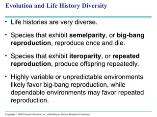
Evolution and Life History Diversity
• Life histories are very diverse.
• Species that exhibit semelparity, or big-bang
reproduction, reproduce once and die.
• Species that exhibit iteroparity, or repeated
reproduction, produce offspring repeatedly.
• Highly variable or unpredictable environments
likely favor big-bang reproduction, while
dependable environments may favor repeated
reproduction.

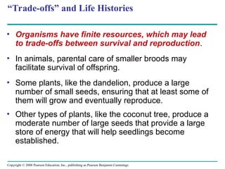
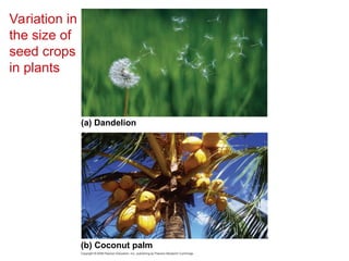
“Trade-offs” and Life Histories
• Organisms have finite resources, which may lead
to trade-offs between survival and reproduction.
• In animals, parental care of smaller broods may
facilitate survival of offspring.
• Some plants, like the dandelion, produce a large
number of small seeds, ensuring that at least some of
them will grow and eventually reproduce.
• Other types of plants, like the coconut tree, produce a
moderate number of large seeds that provide a large
store of energy that will help seedlings become
established.

Variation in
the size of
seed crops
in plants
(a) Dandelion
(b) Coconut palm

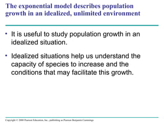
The exponential model describes population
growth in an idealized, unlimited environment
• It is useful to study population growth in an
idealized situation.
• Idealized situations help us understand the
capacity of species to increase and the
conditions that may facilitate this growth.

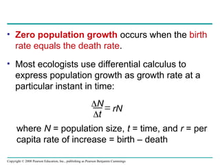
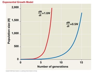
• Zero population growth occurs when the birth
rate equals the death rate.
• Most ecologists use differential calculus to
express population growth as growth rate at a
particular instant in time:
N
t
 rN
where N = population size, t = time, and r = per
capita rate of increase = birth – death

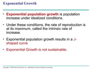
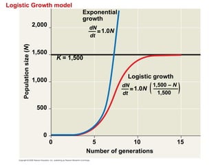
Exponential Growth
• Exponential population growth is population
increase under idealized conditions.
• Under these conditions, the rate of reproduction is
at its maximum, called the intrinsic rate of
increase.
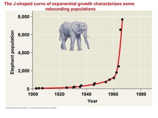
• Exponential population growth results in a J-
shaped curve
• Exponential Growth is not sustainable.

Exponential Growth Model
Number of generations
0 5 10 15
0
500
1,000
1,500
2,000
1.0N
=
dN
dt
0.5N
=
dN
dt
Population
size
(N)

The J-shaped curve of exponential growth characterizes some
rebounding populations
8,000
6,000
4,000
2,000
0
1920 1940 1960 1980
Year
Elephant
population
1900

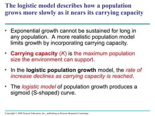
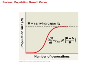
The logistic model describes how a population
grows more slowly as it nears its carrying capacity
• Exponential growth cannot be sustained for long in
any population. A more realistic population model
limits growth by incorporating carrying capacity.
• Carrying capacity (K) is the maximum population
size the environment can support.
• In the logistic population growth model, the rate of
increase declines as carrying capacity is reached.
• The logistic model of population growth produces a
sigmoid (S-shaped) curve.

Logistic Growth model
2,000
1,500
1,000
500
0
0 5 10 15
Population
size
(N)
Exponential
growth
1.0N
=
dN
dt
1.0N
=
dN
dt
K = 1,500
Logistic growth
1,500 – N
1,500

The Logistic Model and Real Populations
• The growth of laboratory populations of
paramecia fits an S-shaped curve.
• These organisms are grown in a constant
environment lacking predators and
competitors.
• Some populations overshoot K before settling
down to a relatively stable density.

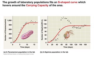
The growth of laboratory populations fits an S-shaped curve which
hovers around the Carrying Capacity of the area.
1,000
800
600
400
200
0
0 5 10 15
Time (days)
Number
of
Paramecium/mL
Number
of
Daphnia/50
mL
0
30
60
90
180
150
120
0 20 40 60 80 100 120 140 160
Time (days)
(b) A Daphnia population in the lab
(a) A Paramecium population in the lab

The Logistic Model and Life Histories
• Life history traits favored by natural selection
may vary with population density and
environmental conditions.
• K-selection = density-dependent selection,
selects for life history traits that are sensitive to
population density.
• r-selection = or density-independent
selection, selects for life history traits that
maximize reproduction.

Many factors that regulate population growth are
density dependent
• There are two general questions about
regulation of population growth:
– What environmental factors stop a population
from growing indefinitely?
– Why do some populations show radical
fluctuations in size over time, while others
remain stable?

Population Change and Population Density
• In density-independent populations, birth rate
and death rate do not change with population
density.
• In density-dependent populations, birth rates
fall and death rates rise with population
density.

Density-Dependent Population Regulation
• Density-dependent birth and death rates are
an example of negative feedback that regulates
population growth.
• They are affected by many factors, such as
competition for resources, territoriality, disease,
predation, toxic wastes, and intrinsic factors.
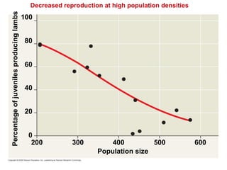
• In crowded populations, increasing population
density intensifies competition for resources
and results in a lower birth rate.

Decreased reproduction at high population densities
Population size
100
80
60
40
20
0
200 400 500 600
300
Percentage
of
juveniles
producing
lambs

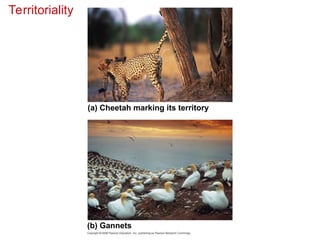
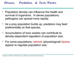
Territoriality
• In many vertebrates and some invertebrates,
competition for territory may limit density.
• Cheetahs are highly territorial, using chemical
communication to warn other cheetahs of their
boundaries.

Territoriality
(a) Cheetah marking its territory
(b) Gannets

Disease, Predation, & Toxic Wastes
• Population density can influence the health and
survival of organisms. In dense populations,
pathogens can spread more rapidly.
• As a prey population builds up, predators may feed
preferentially on that species.
• Accumulation of toxic wastes can contribute to
density-dependent regulation of population size.
• For some populations, intrinsic (physiological) factors
appear to regulate population size.

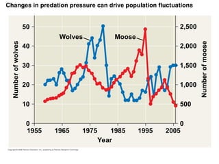
Population Dynamics
• The study of population dynamics focuses on
the complex interactions between biotic and
abiotic factors that cause variation in
population size.
• Long-term population studies have challenged
the hypothesis that populations of large
mammals are relatively stable over time.
• Weather can affect population size over time.

Changes in predation pressure can drive population fluctuations
Wolves Moose
2,500
2,000
1,500
1,000
500
Number
of
moose
0
Number
of
wolves
50
40
30
20
10
0
1955 1965 1975 1985 1995 2005
Year

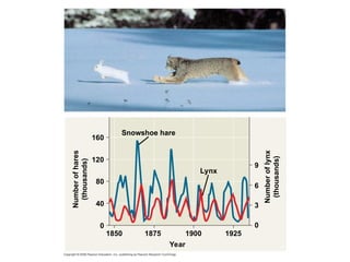
Population Cycles: Scientific Inquiry
• Some populations undergo regular boom-and-
bust cycles.
• Lynx populations follow the 10 year boom-and-
bust cycle of hare populations.
• Three hypotheses have been proposed to
explain the hare’s 10-year interval.

Snowshoe hare
Lynx
Number
of
lynx
(thousands)
Number
of
hares
(thousands)
160
120
80
40
0
1850 1875 1900 1925
Year
9
6
3
0

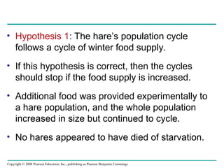
• Hypothesis 1: The hare’s population cycle
follows a cycle of winter food supply.
• If this hypothesis is correct, then the cycles
should stop if the food supply is increased.
• Additional food was provided experimentally to
a hare population, and the whole population
increased in size but continued to cycle.
• No hares appeared to have died of starvation.

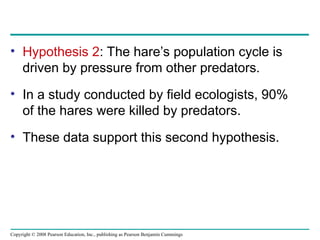
• Hypothesis 2: The hare’s population cycle is
driven by pressure from other predators.
• In a study conducted by field ecologists, 90%
of the hares were killed by predators.
• These data support this second hypothesis.

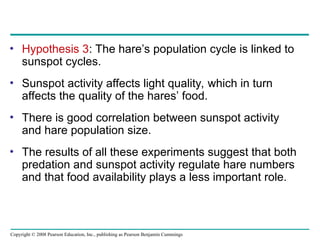
• Hypothesis 3: The hare’s population cycle is linked to
sunspot cycles.
• Sunspot activity affects light quality, which in turn
affects the quality of the hares’ food.
• There is good correlation between sunspot activity
and hare population size.
• The results of all these experiments suggest that both
predation and sunspot activity regulate hare numbers
and that food availability plays a less important role.

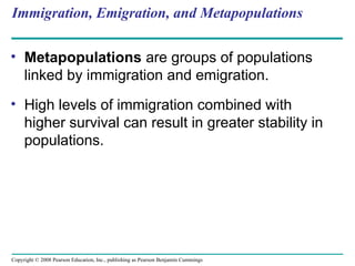
Immigration, Emigration, and Metapopulations
• Metapopulations are groups of populations
linked by immigration and emigration.
• High levels of immigration combined with
higher survival can result in greater stability in
populations.

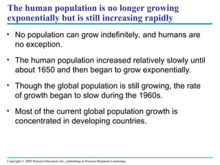
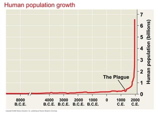
The human population is no longer growing
exponentially but is still increasing rapidly
• No population can grow indefinitely, and humans are
no exception.
• The human population increased relatively slowly until
about 1650 and then began to grow exponentially.
• Though the global population is still growing, the rate
of growth began to slow during the 1960s.
• Most of the current global population growth is
concentrated in developing countries.

Human population growth
8000
B.C.E.
4000
B.C.E.
3000
B.C.E.
2000
B.C.E.
1000
B.C.E.
0 1000
C.E.
2000
C.E.
0
1
2
3
4
5
6
The Plague
Human
population
(billions)
7

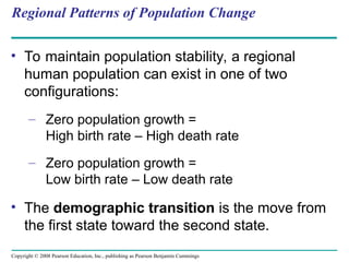
Regional Patterns of Population Change
• To maintain population stability, a regional
human population can exist in one of two
configurations:
– Zero population growth =
High birth rate – High death rate
– Zero population growth =
Low birth rate – Low death rate
• The demographic transition is the move from
the first state toward the second state.

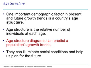
Age Structure
• One important demographic factor in present
and future growth trends is a country’s age
structure.
• Age structure is the relative number of
individuals at each age.
• Age structure diagrams can predict a
population’s growth trends.
• They can illuminate social conditions and help
us plan for the future.

Age-structure pyramids for the human population of
three countries
Rapid growth
Afghanistan
Male Female Age Age
Male Female
Slow growth
United States
Male Female
No growth
Italy
85+
80–84
75–79
70–74
60–64
65–69
55–59
50–54
45–49
40–44
35–39
30–34
25–29
20–24
15–19
0–4
5–9
10–14
85+
80–84
75–79
70–74
60–64
65–69
55–59
50–54
45–49
40–44
35–39
30–34
25–29
20–24
15–19
0–4
5–9
10–14
10 10
8 8
6
6 4 4
2
2 0
Percent of population Percent of population Percent of population
6
6 4 4
2
2 0
8 8 6
6 4 4
2
2 0
8 8

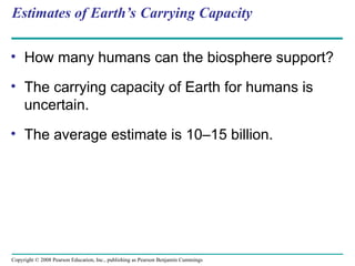
Estimates of Earth’s Carrying Capacity
• How many humans can the biosphere support?
• The carrying capacity of Earth for humans is
uncertain.
• The average estimate is 10–15 billion.

Limits on Human Population Size
• The ecological footprint concept summarizes the
aggregate land and water area needed to sustain the
people of a nation.
• It is one measure of how close we are to the carrying
capacity of Earth.
• Countries vary greatly in footprint size and available
ecological capacity.
• Our carrying capacity could potentially be limited by
food, space, nonrenewable resources, or buildup of
wastes.

Review: Population Growth Curve
K = carrying capacity
Population
size
(N)
rmax N
dN
dt
=
K – N
K

You should now be able to:
1. Define and distinguish between the following
sets of terms: density and dispersion;
clumped dispersion, uniform dispersion, and
random dispersion; life table and reproductive
table; Type I, Type II, and Type III
survivorship curves; semelparity and
iteroparity; r-selected populations and K-
selected populations.
2. Explain how ecologists may estimate the
density of a species.

3. Explain how limited resources and trade-offs
may affect life histories.
4. Compare the exponential and logistic models
of population growth.
5. Explain how density-dependent and density-
independent factors may affect population
growth.
6. Explain how biotic and abiotic factors may
work together to control a population’s growth.

the population ecology 53_lecture_presentation_0.ppt

More Related Content

Similar to the population ecology 53_lecture_presentation_0.ppt

More from khalidmr1830

Recently uploaded

the population ecology 53_lecture_presentation_0.ppt

Editor's Notes