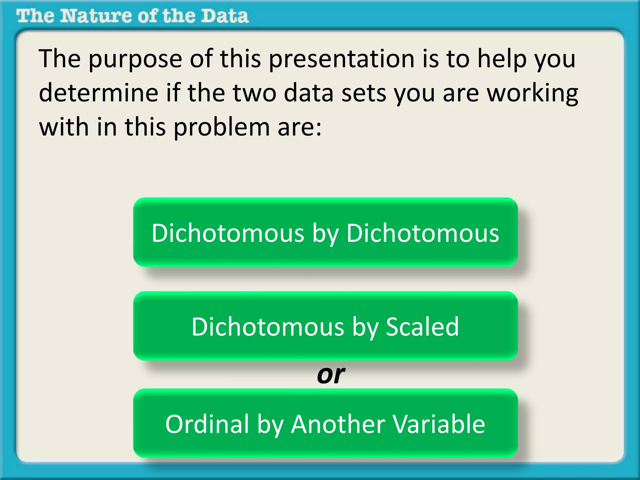
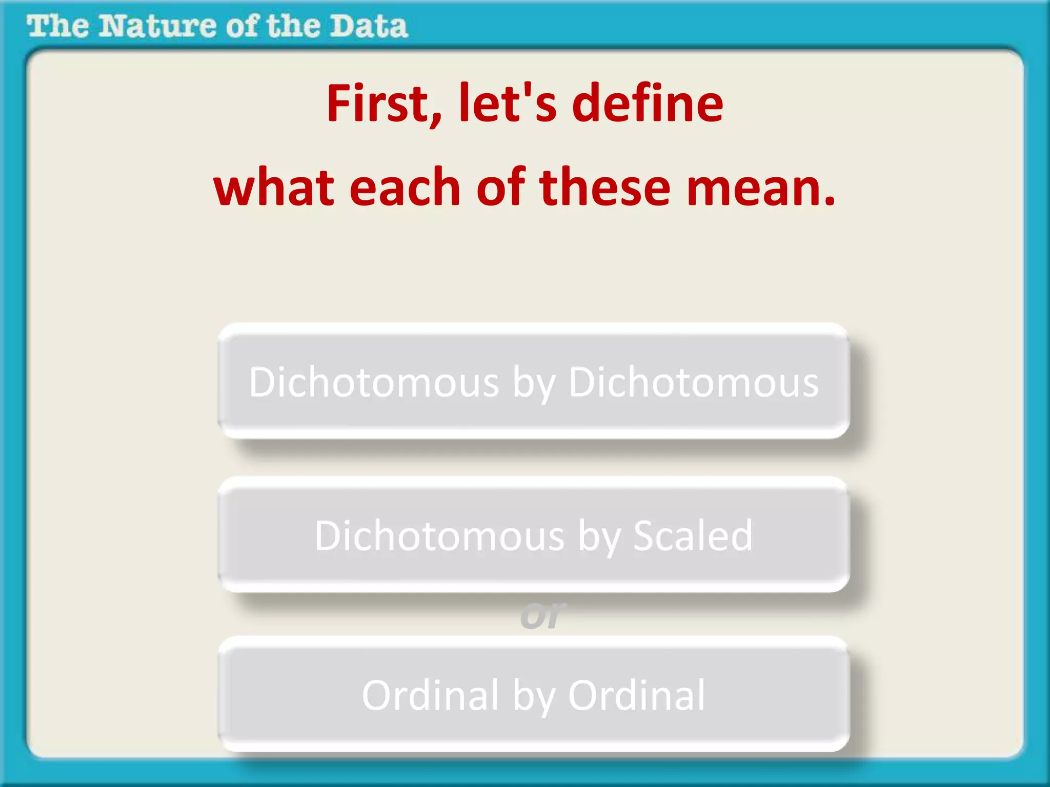
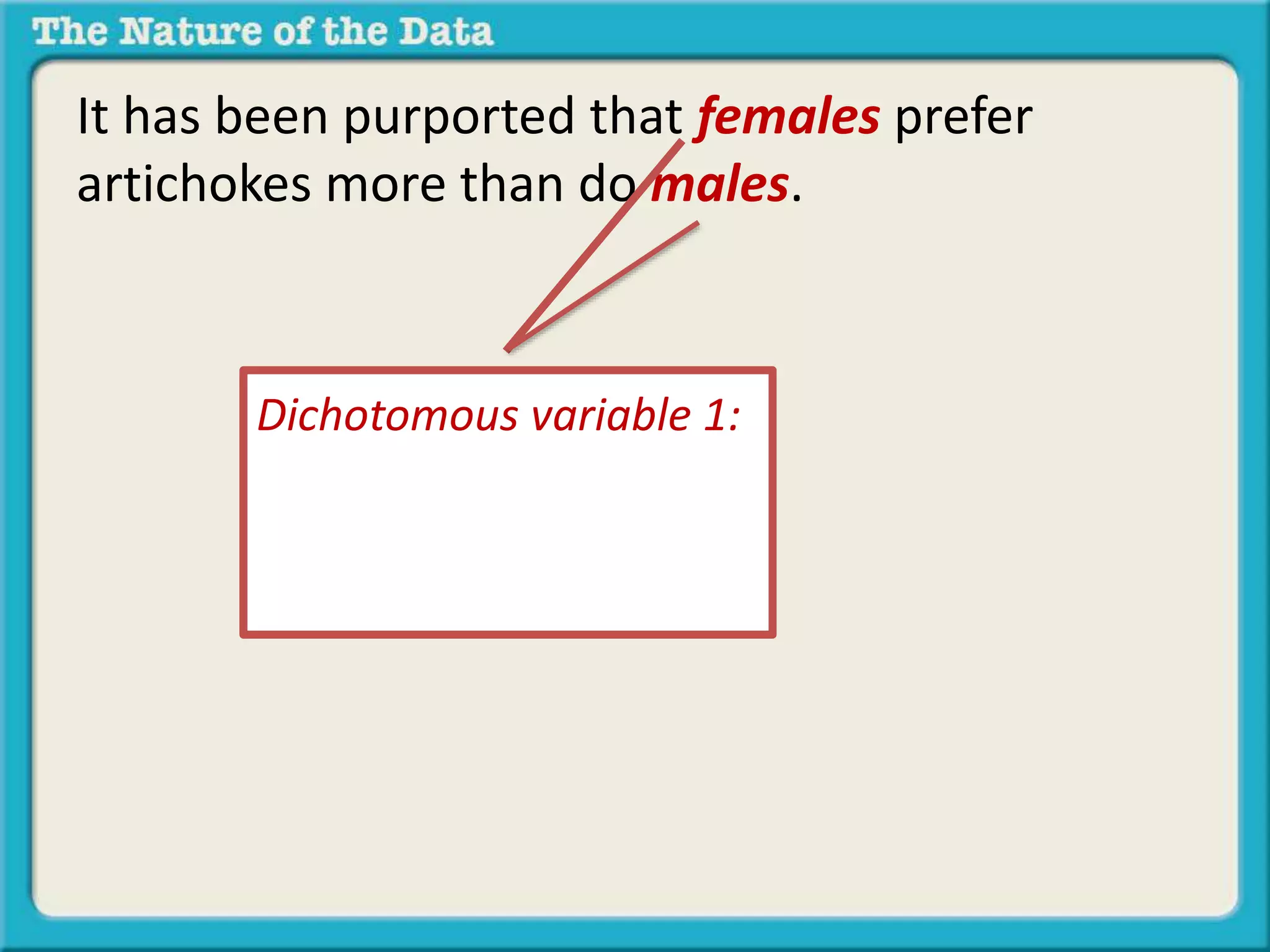
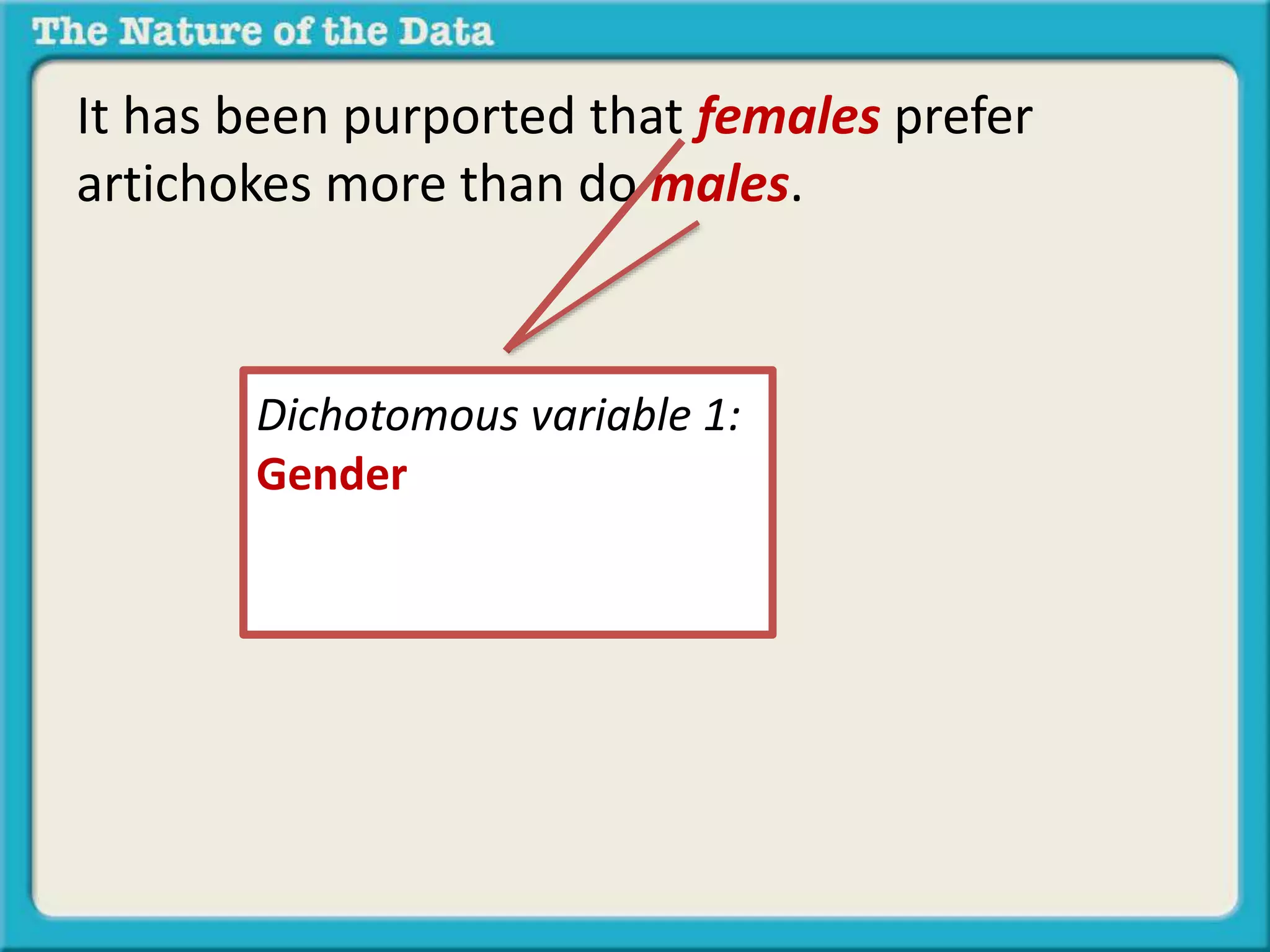
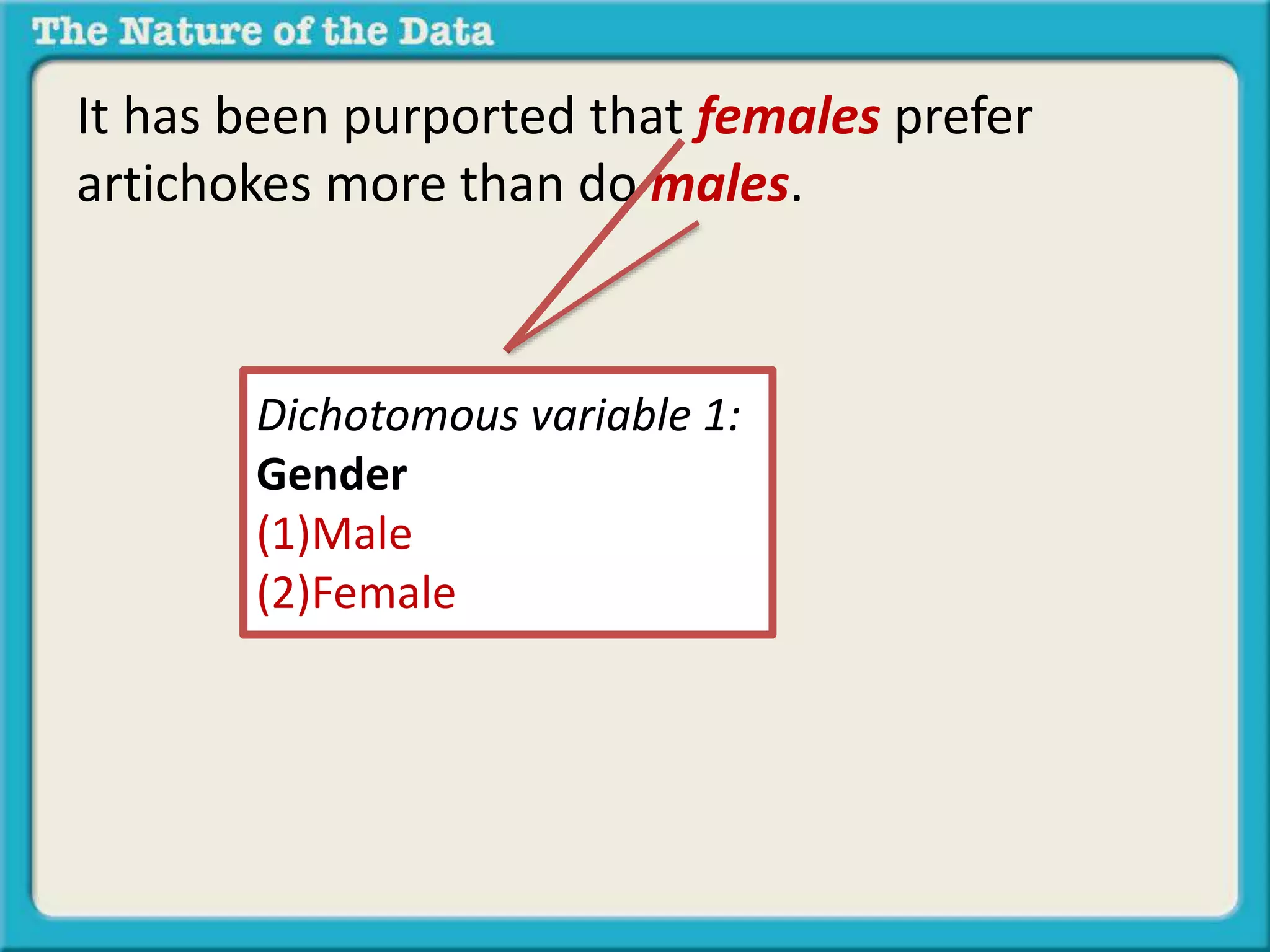
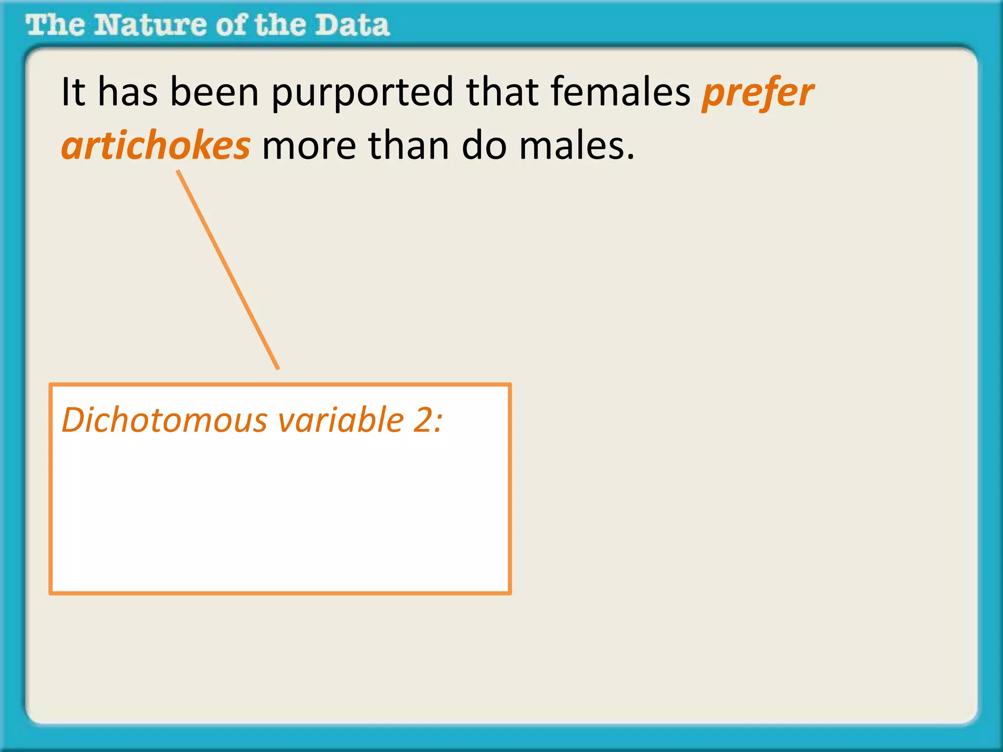
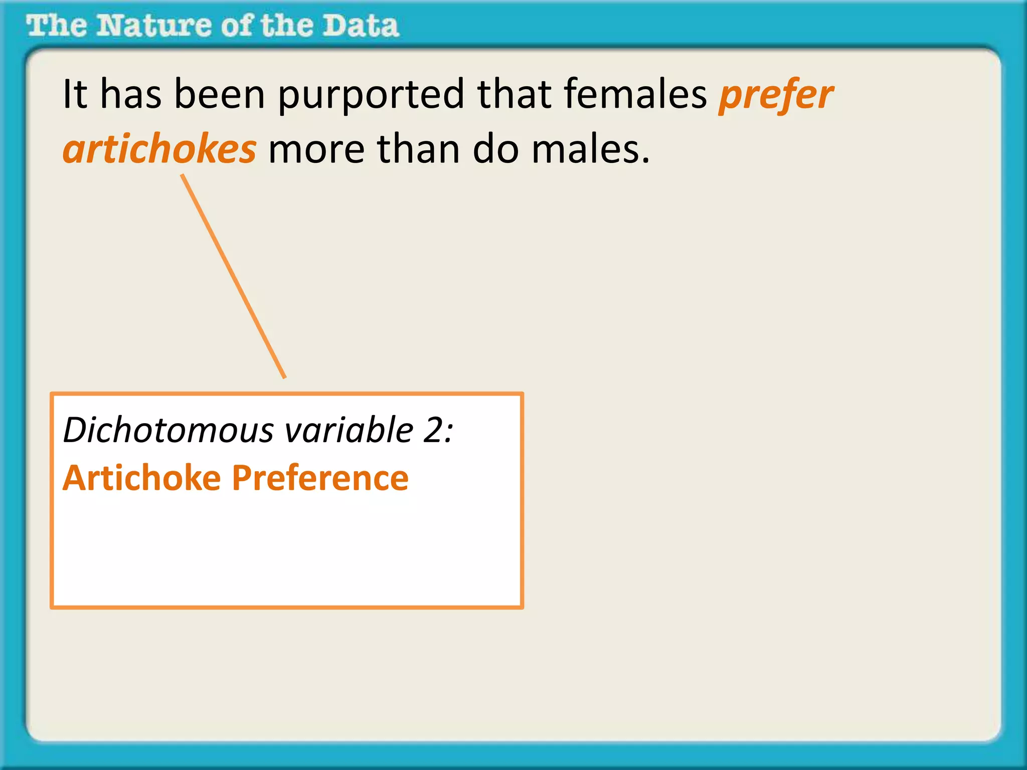
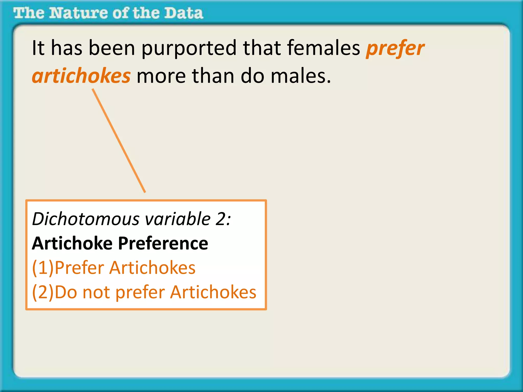
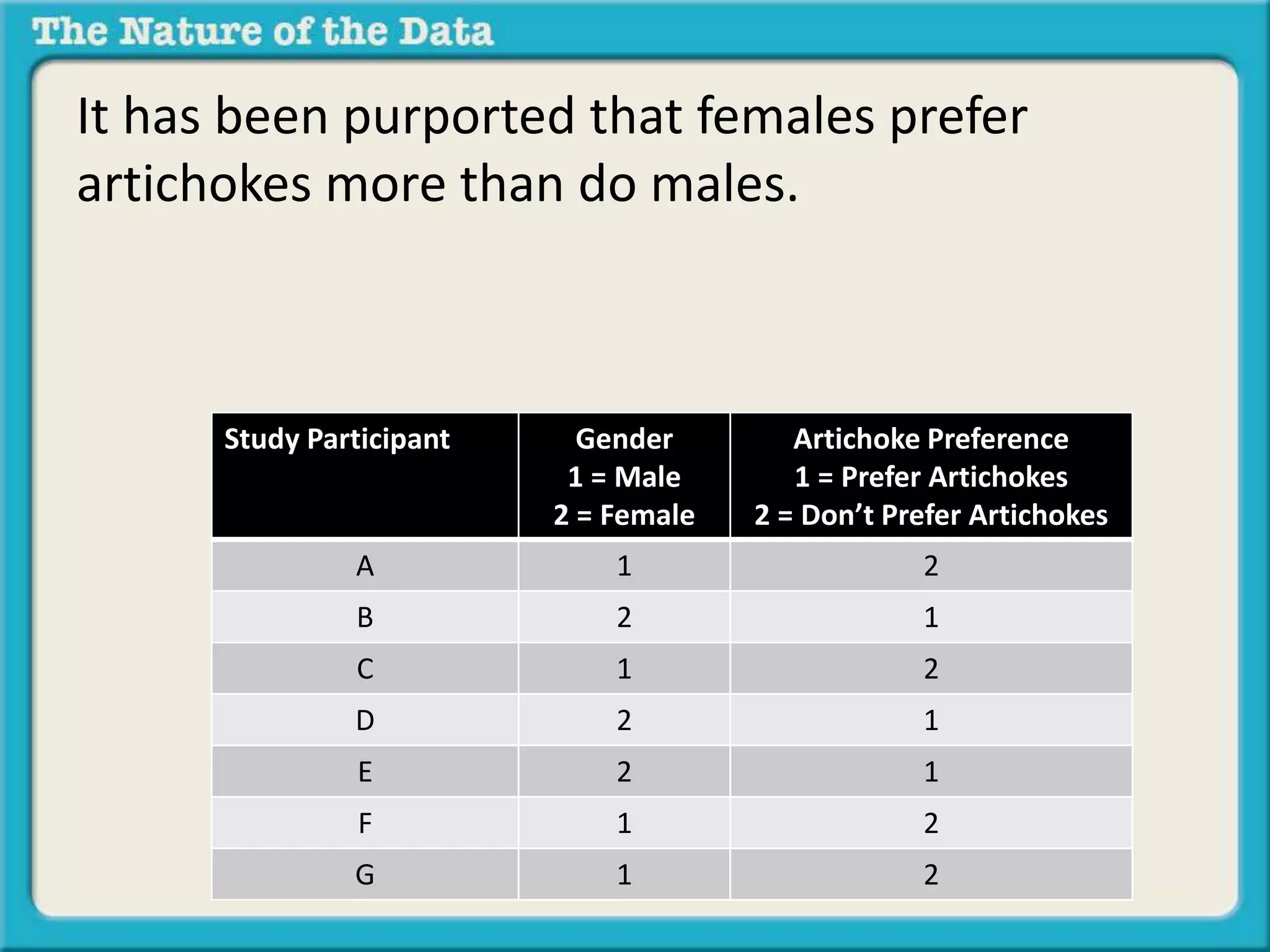
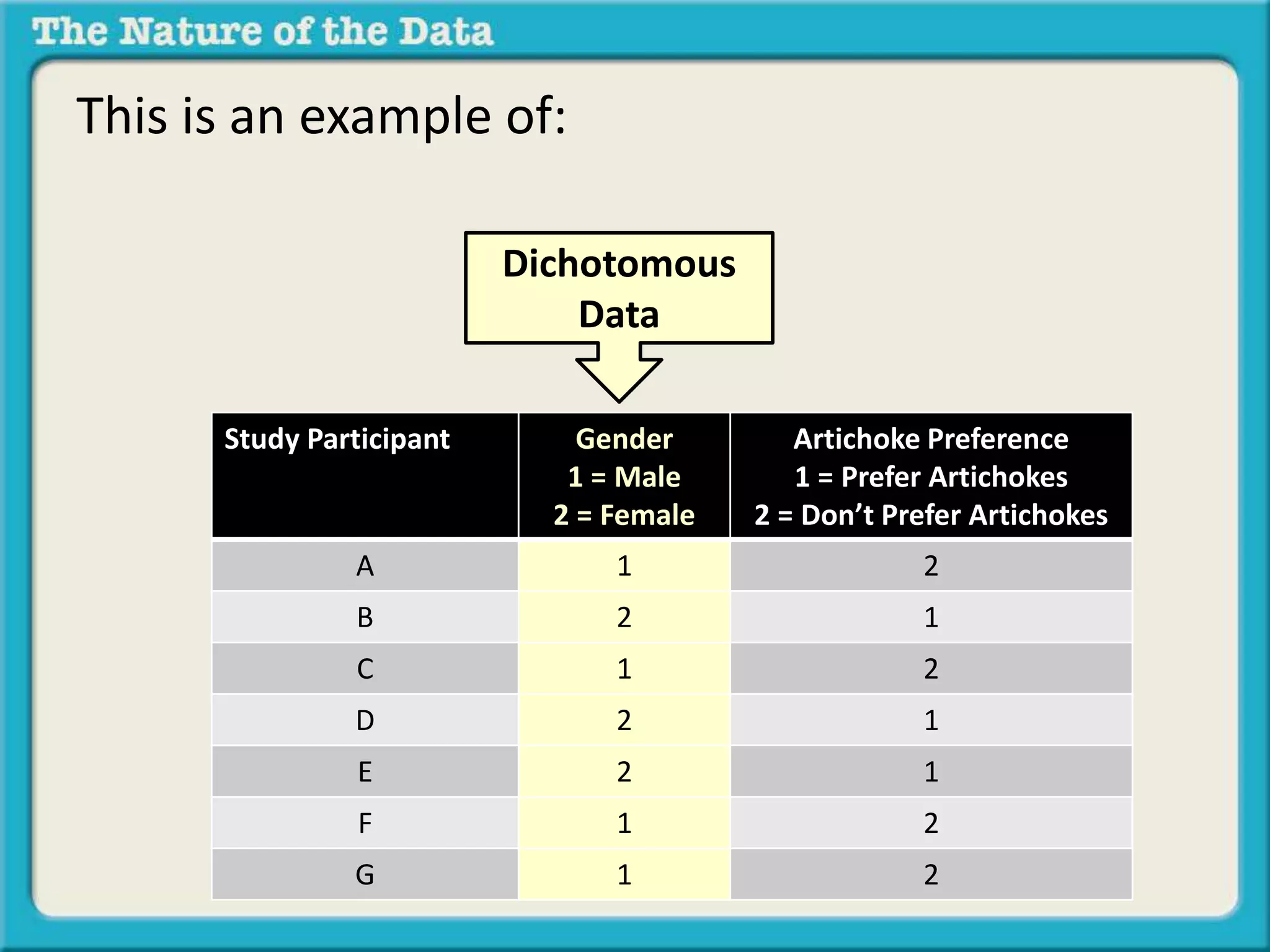
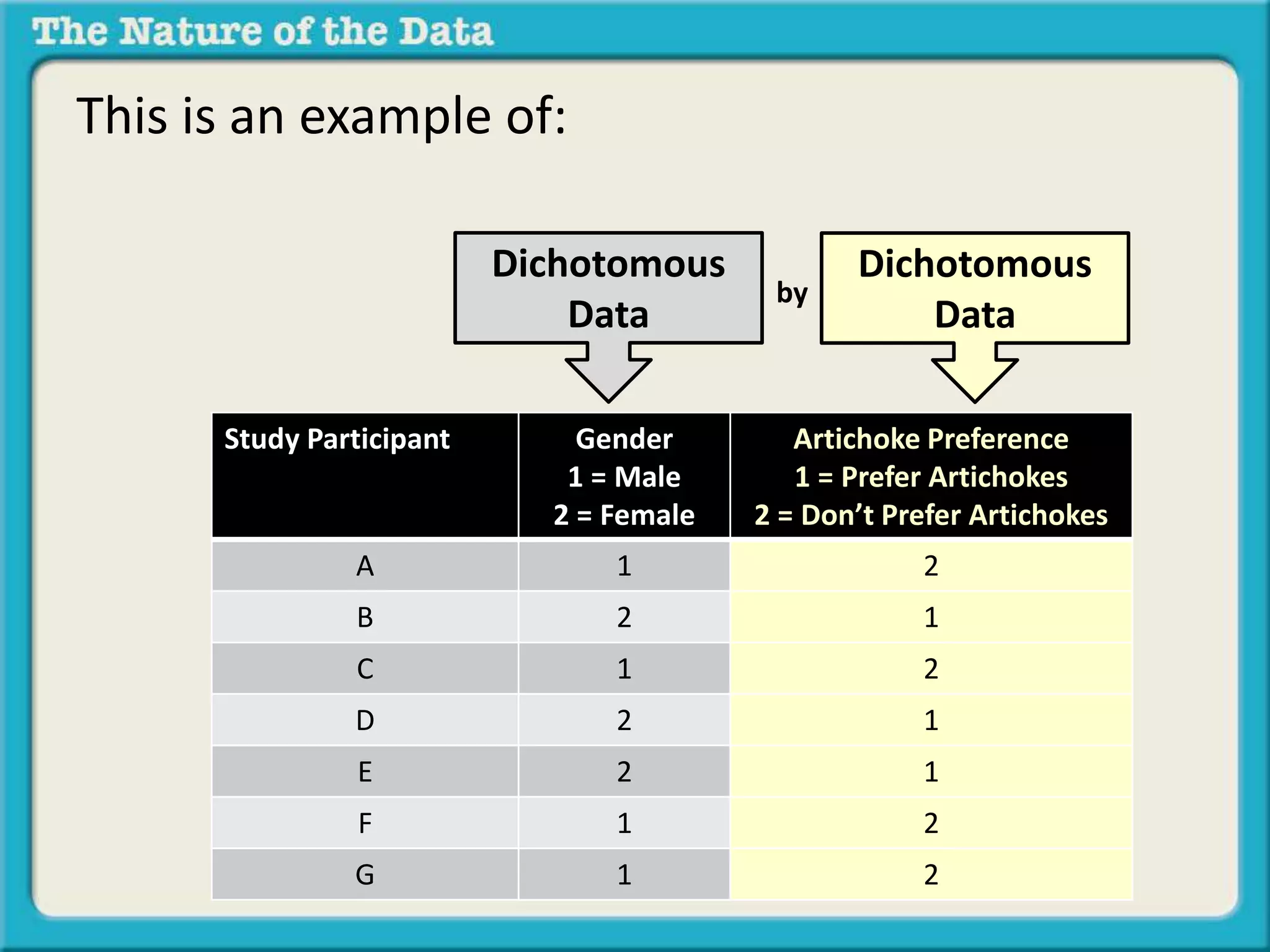
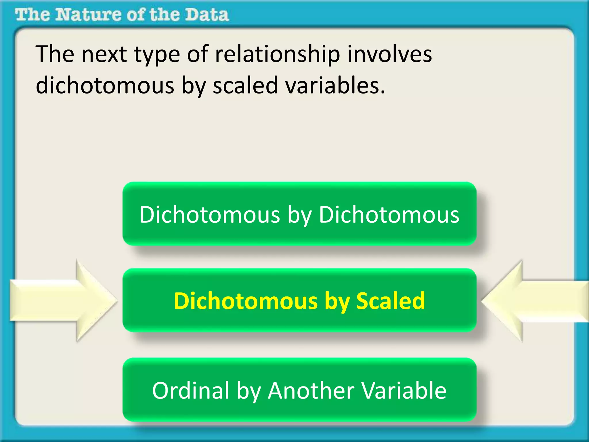
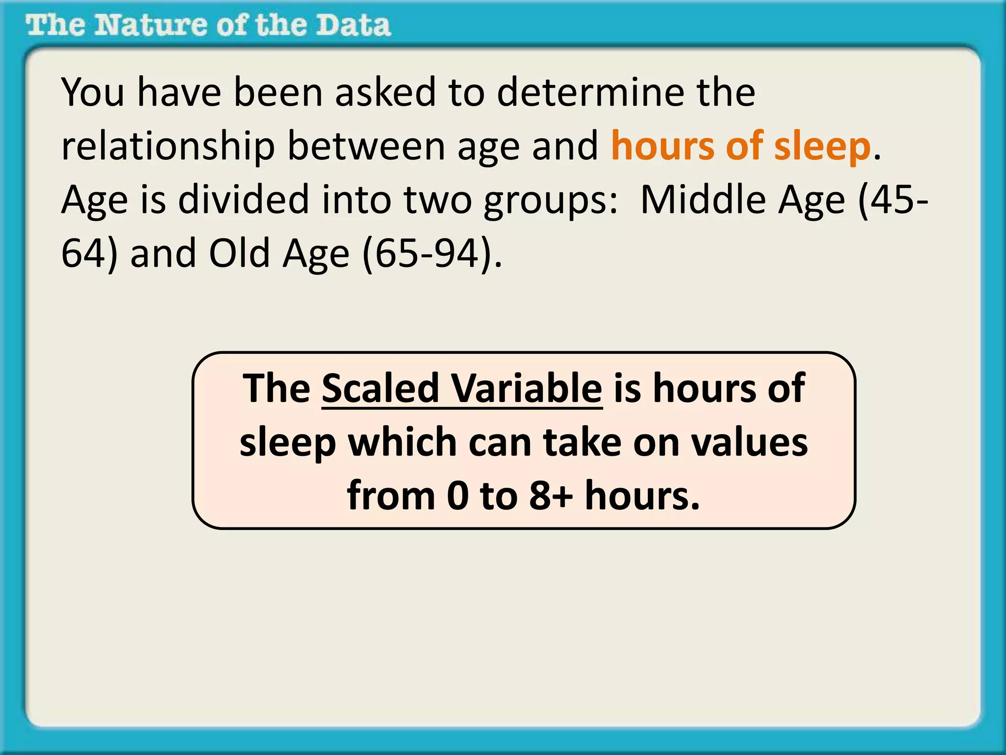
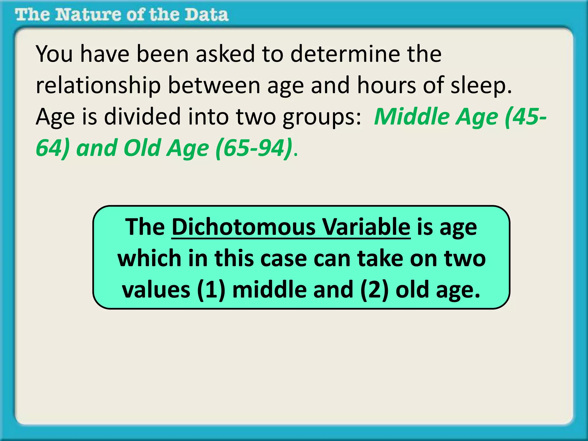
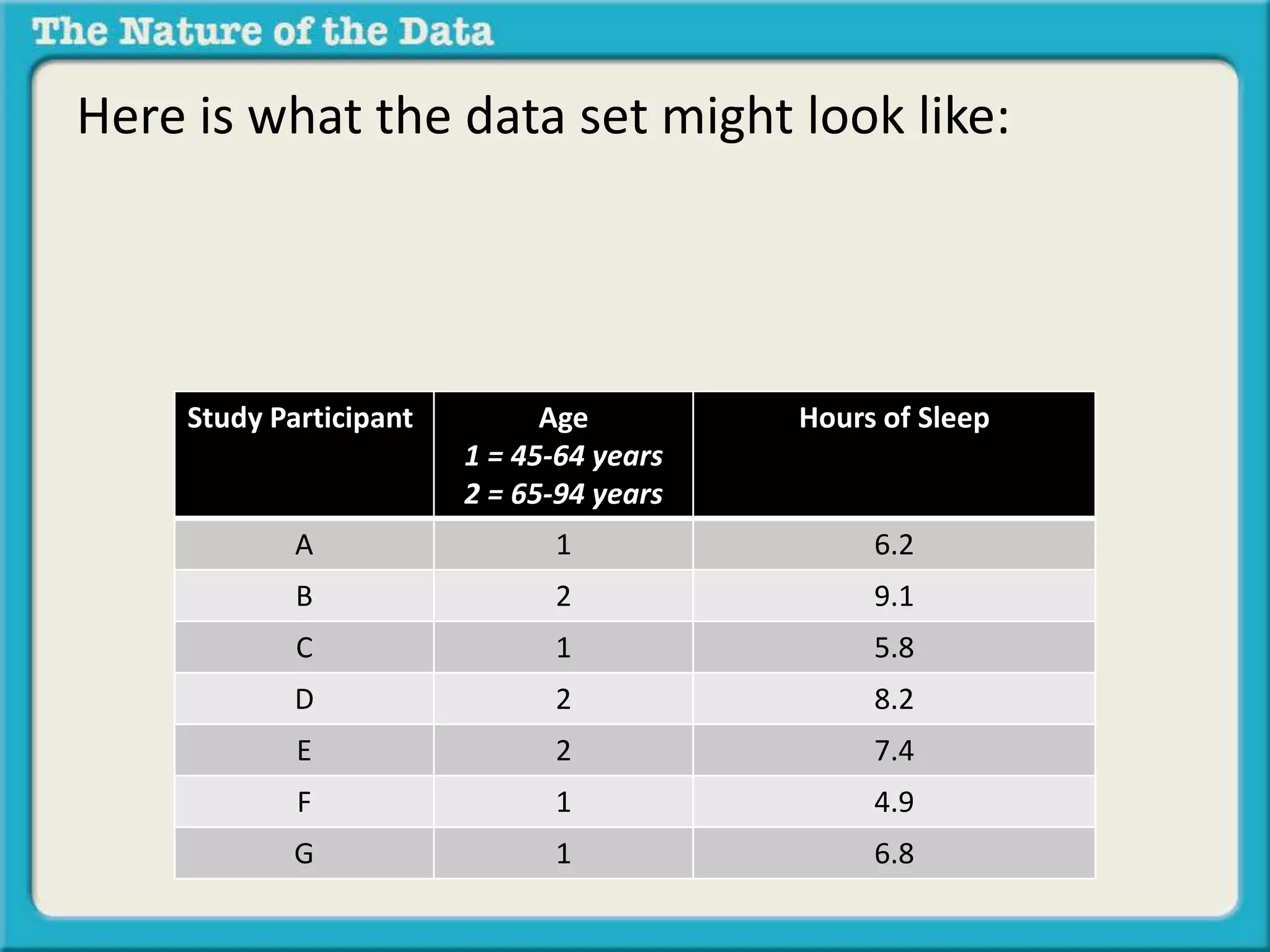
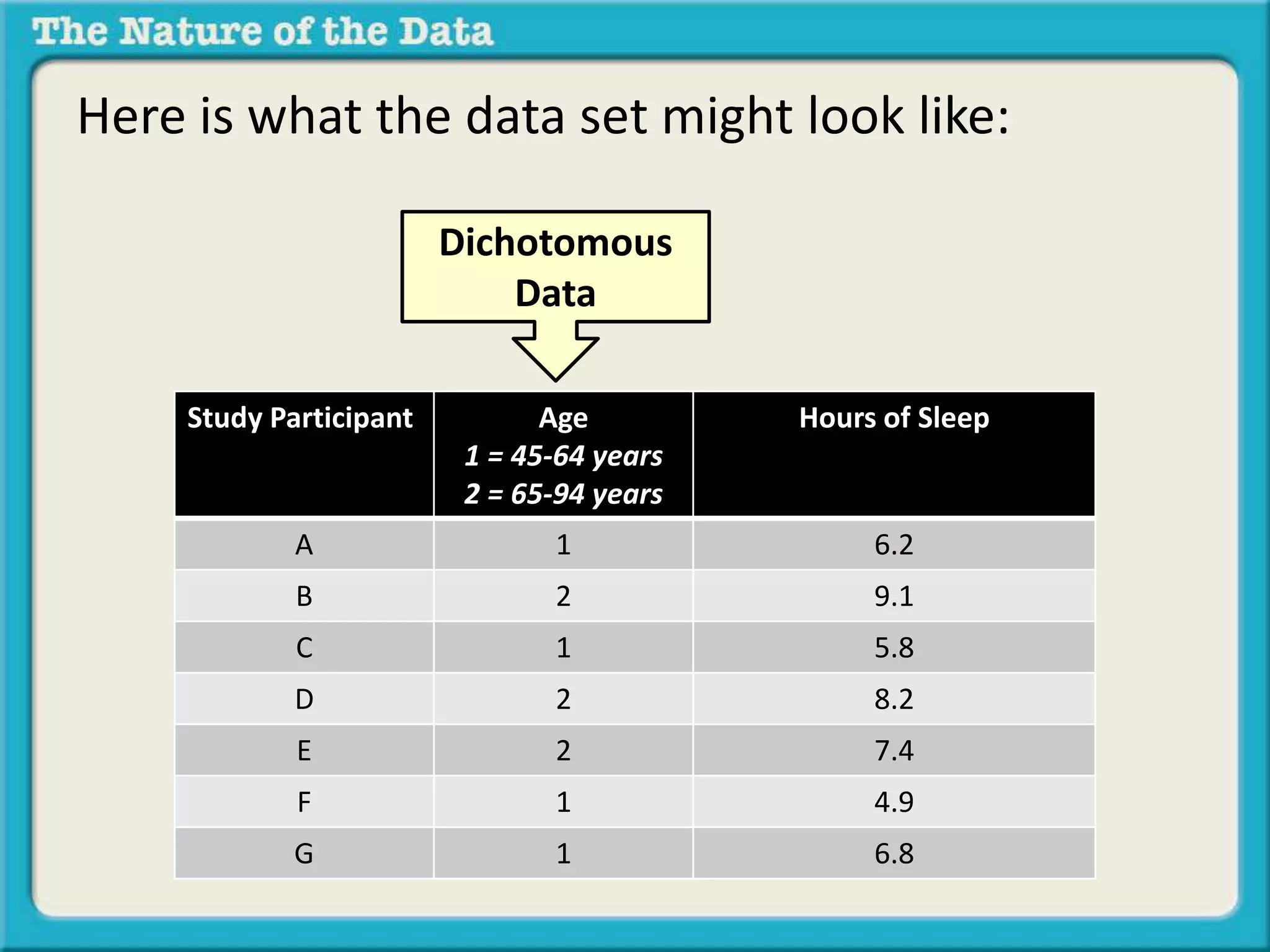
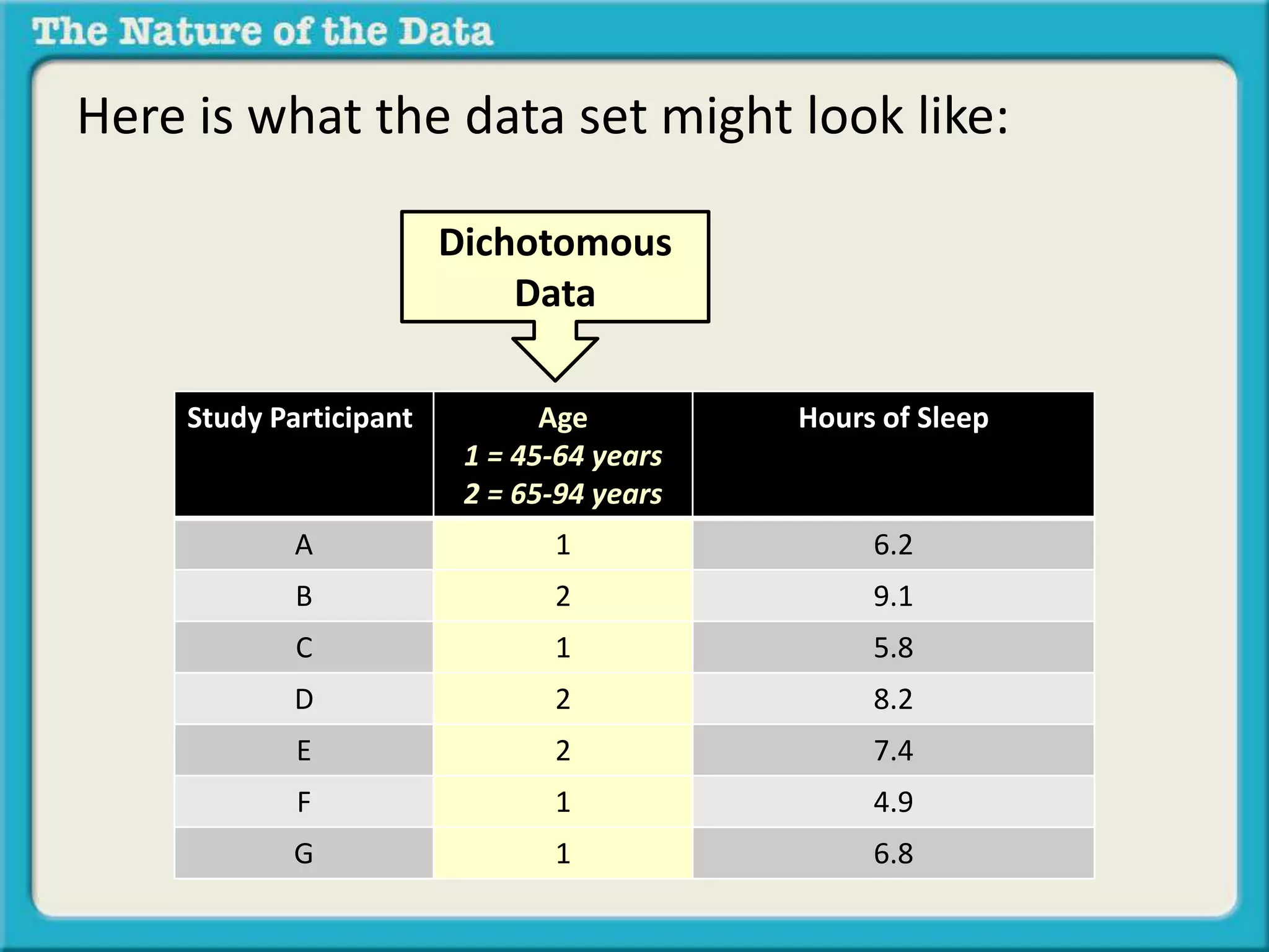
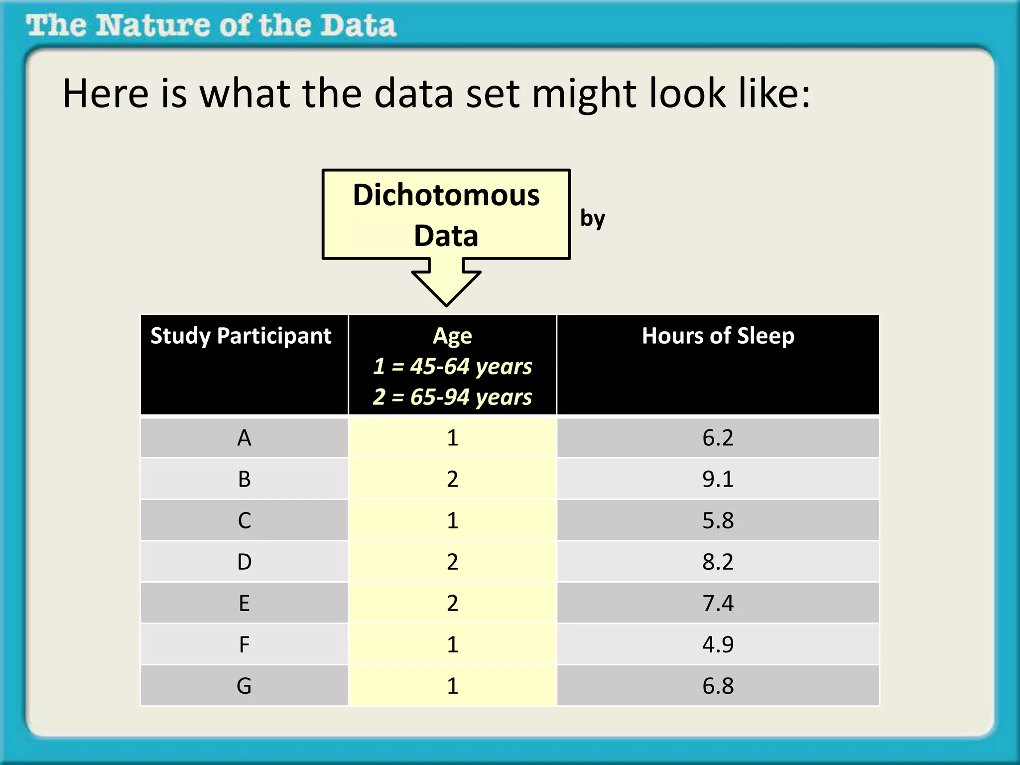
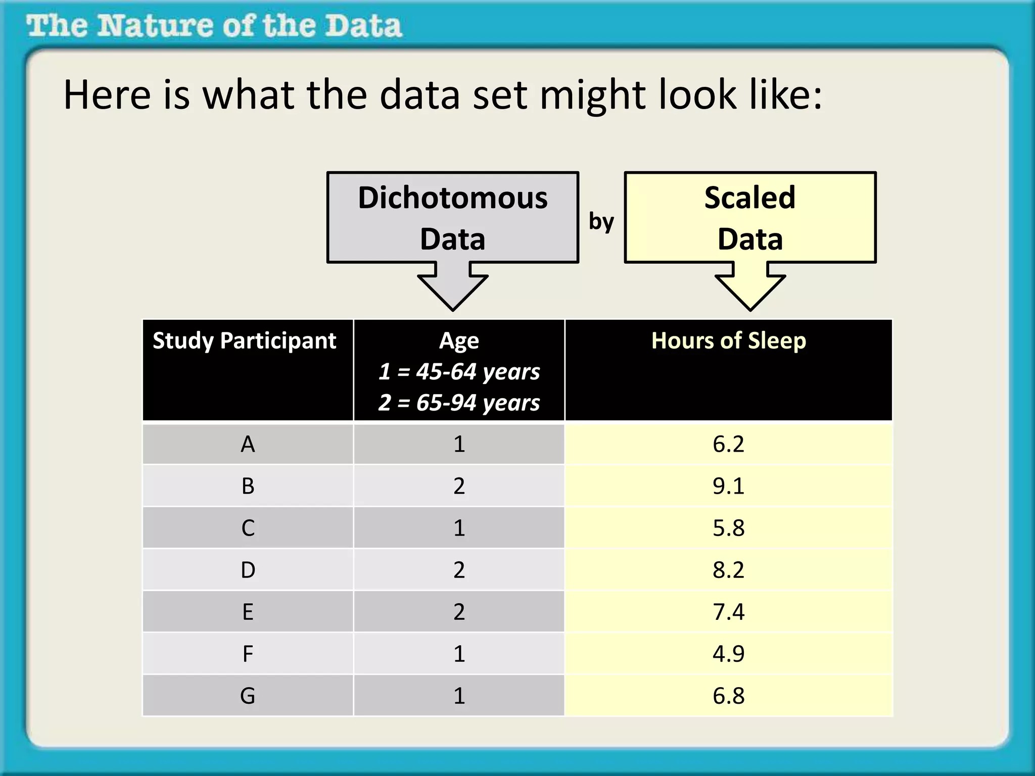
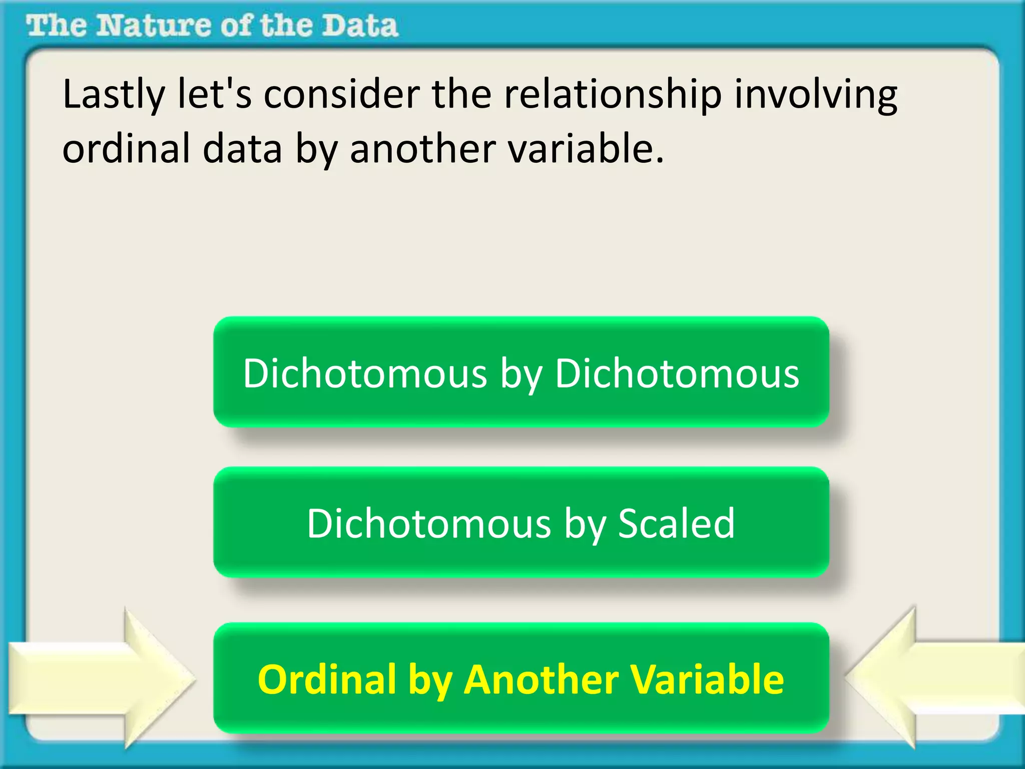
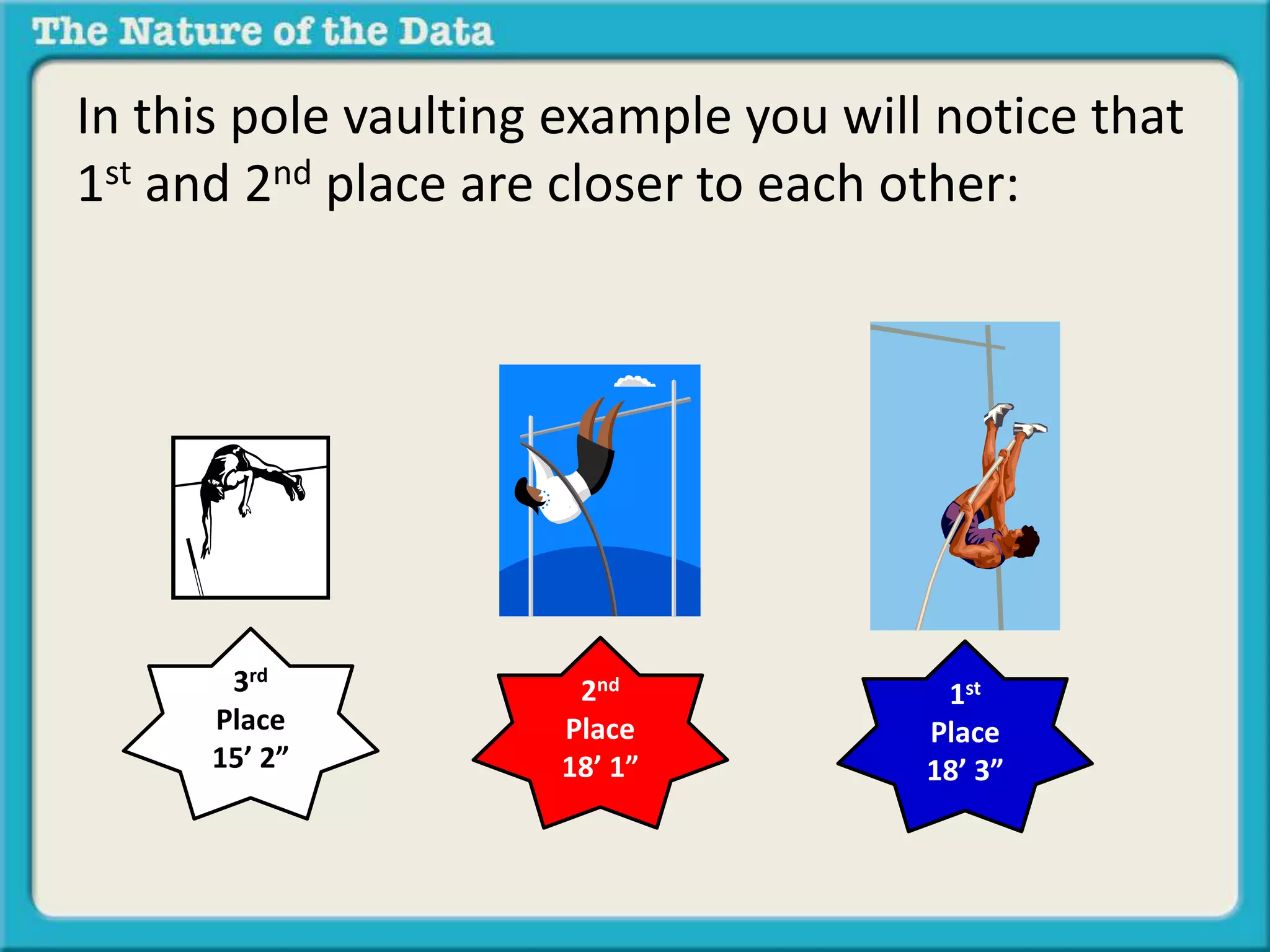
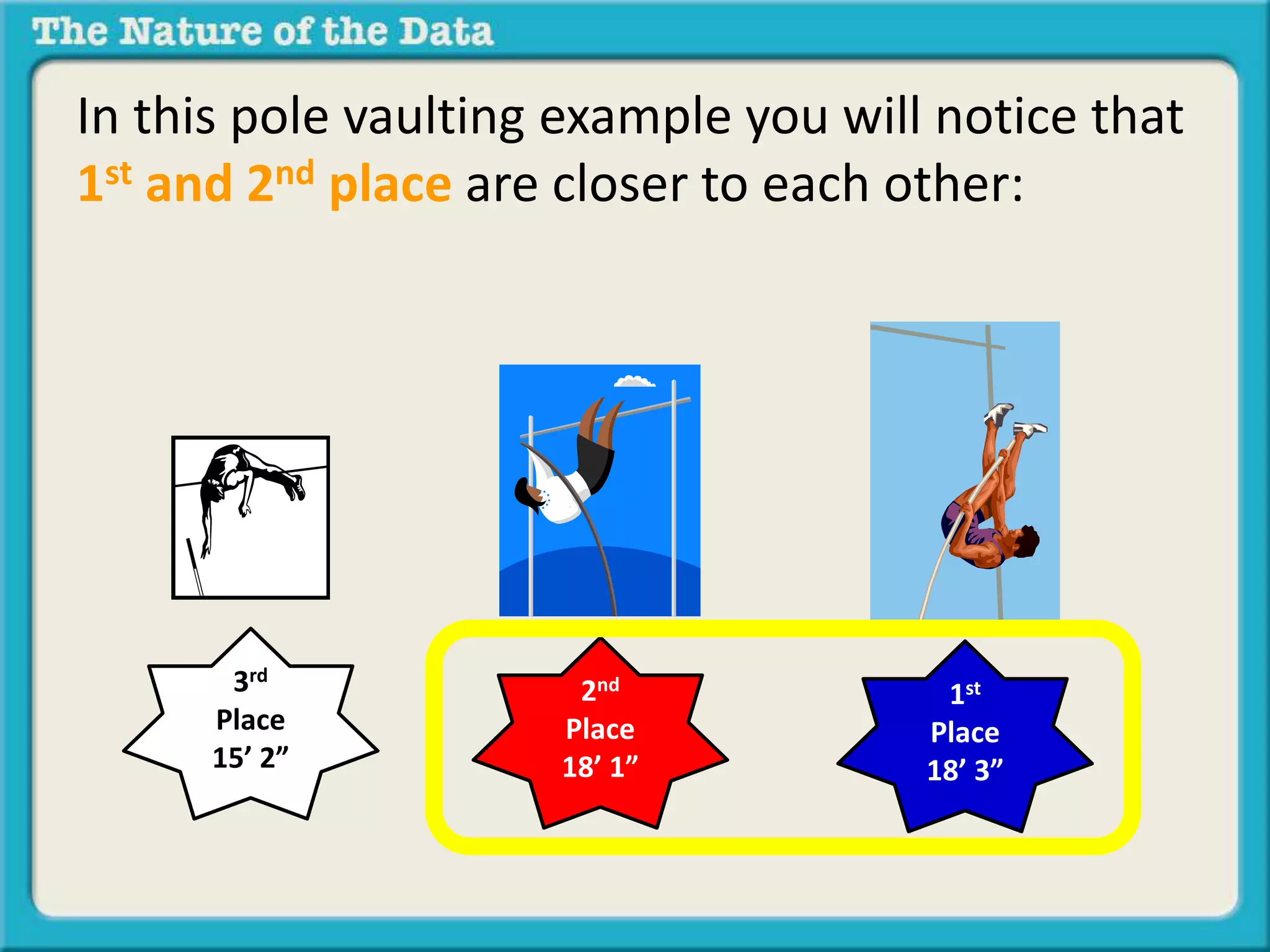
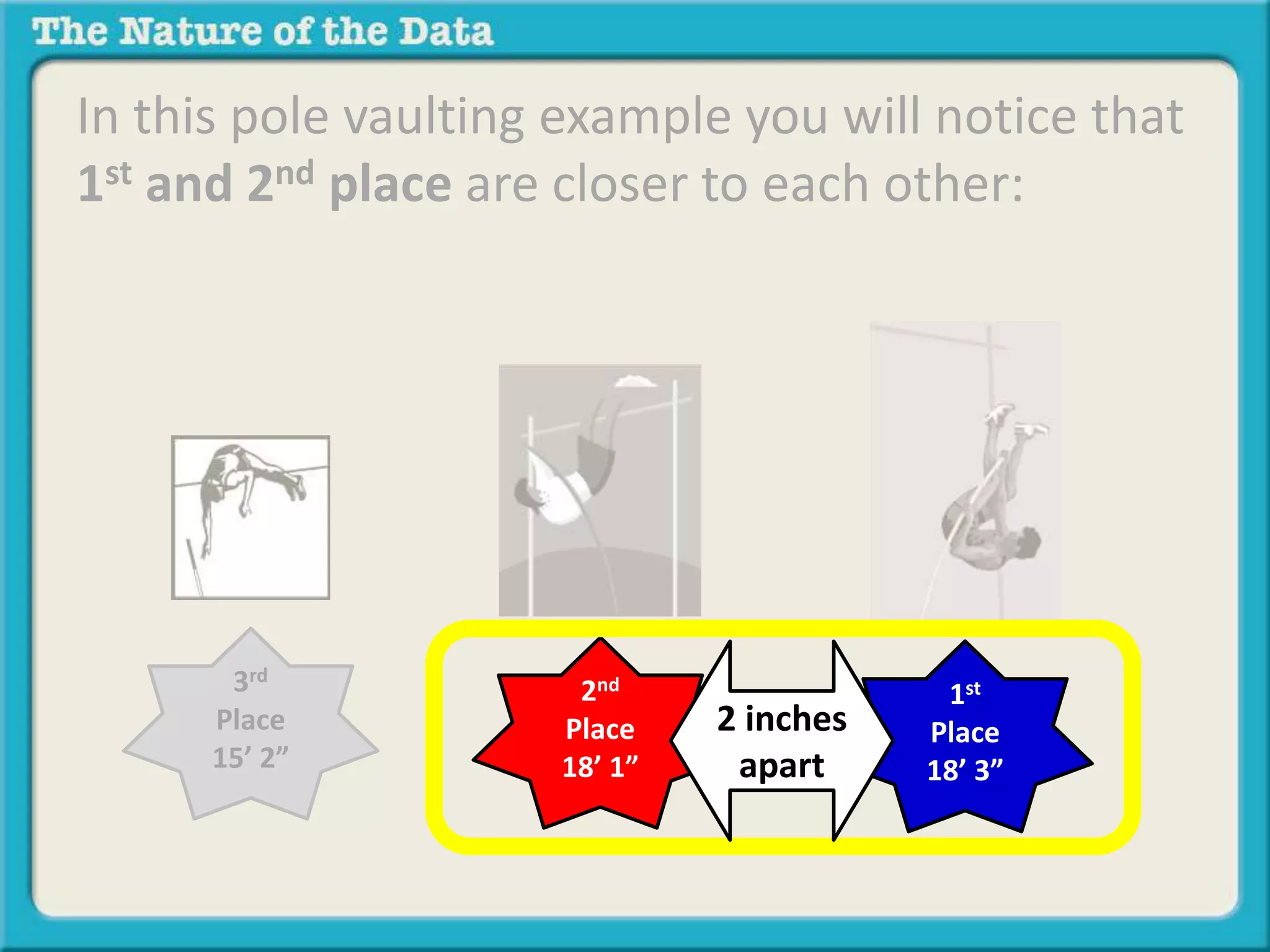
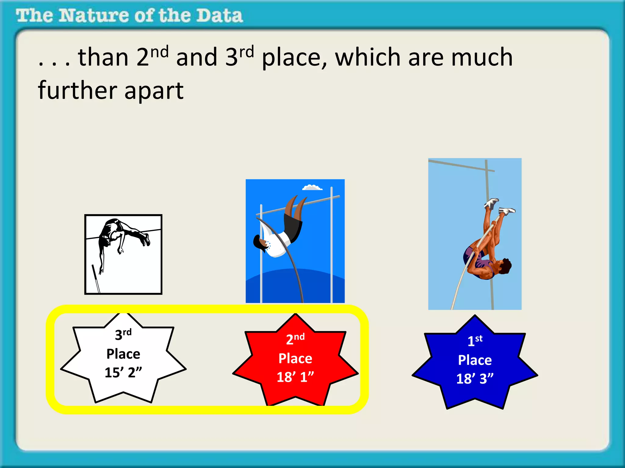
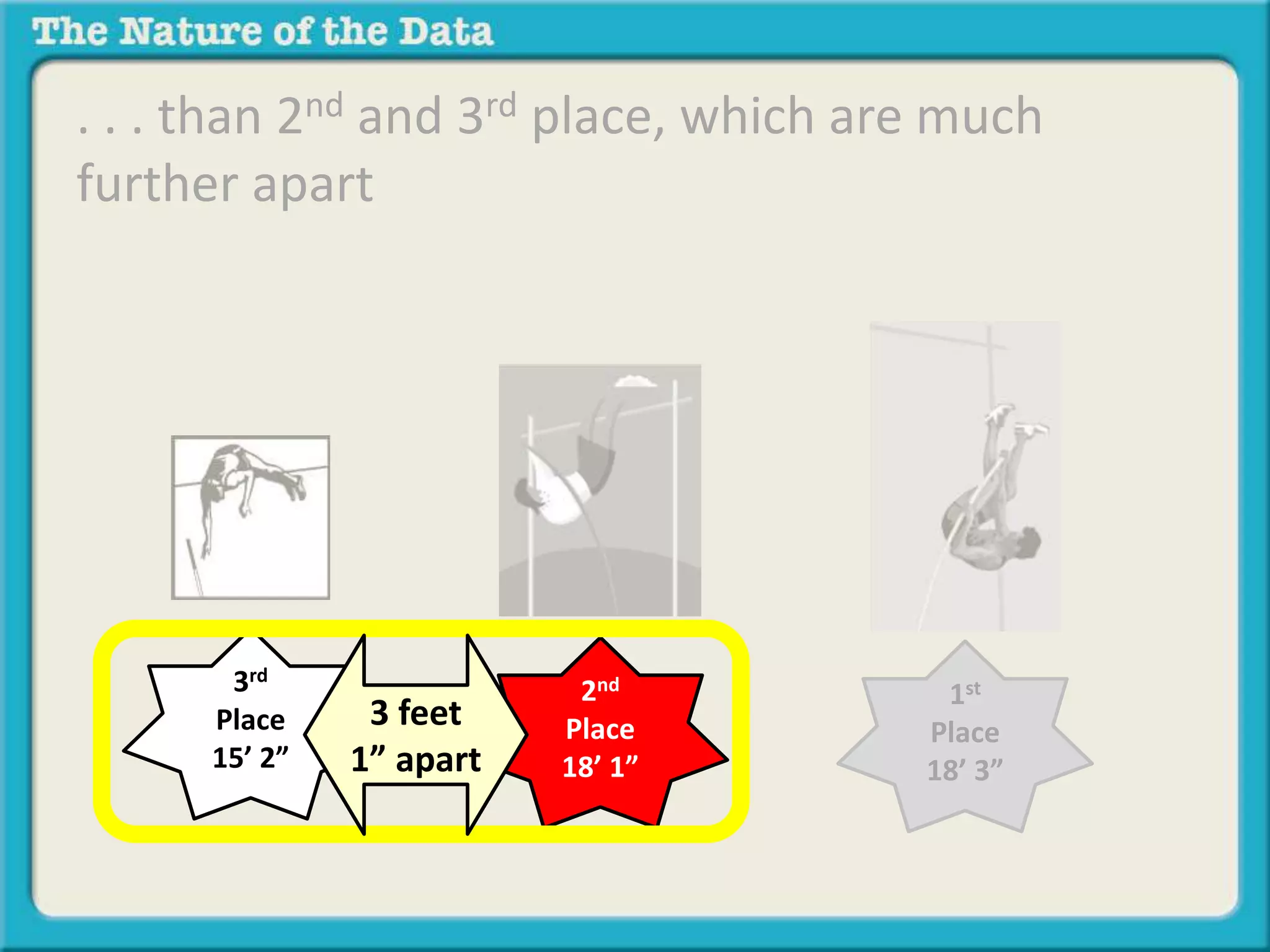
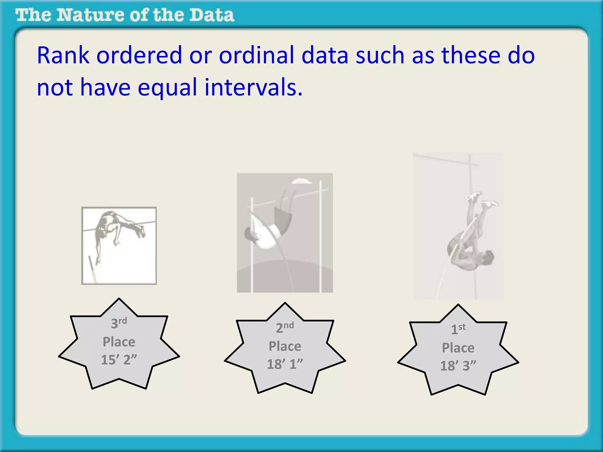
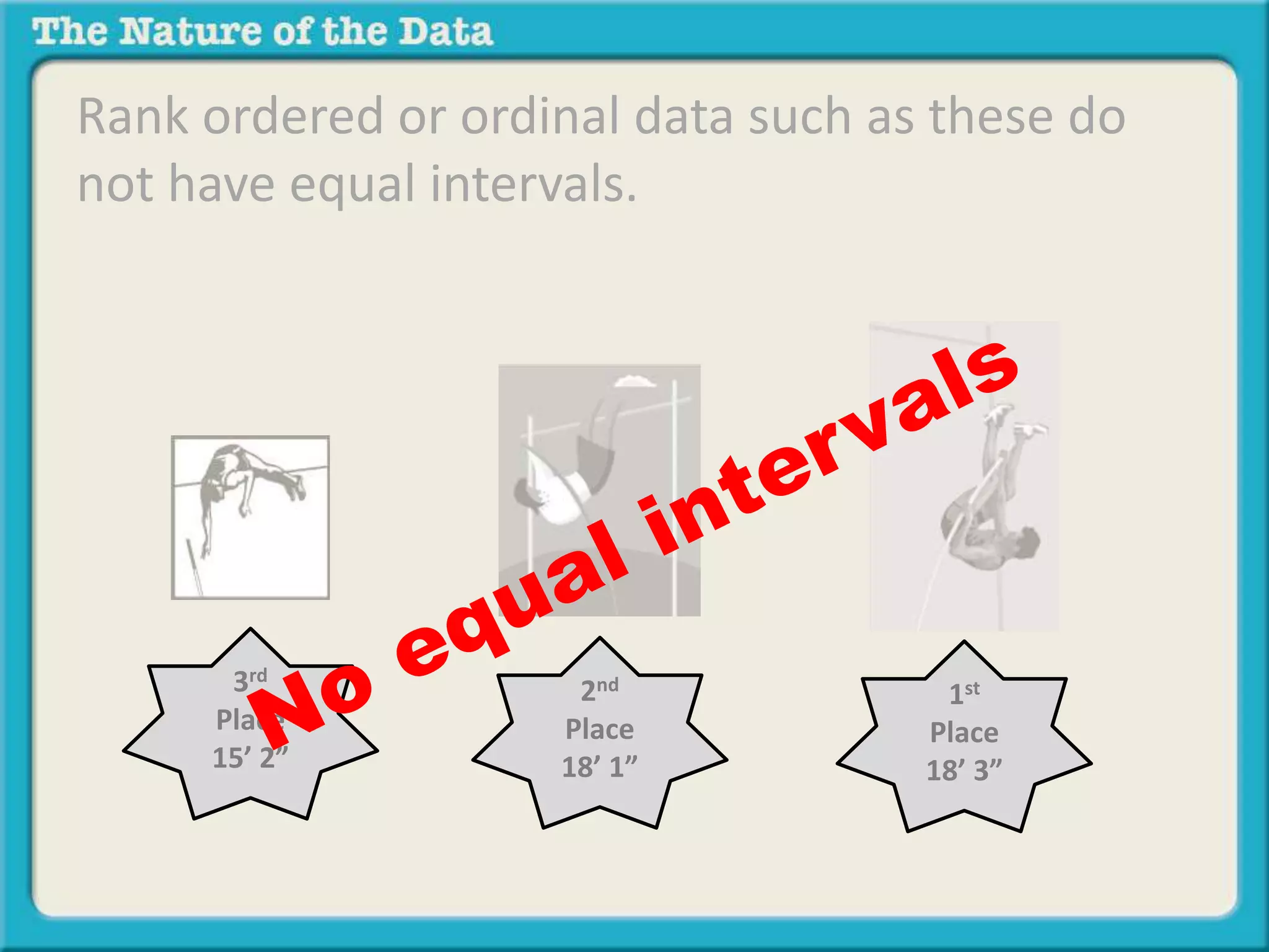
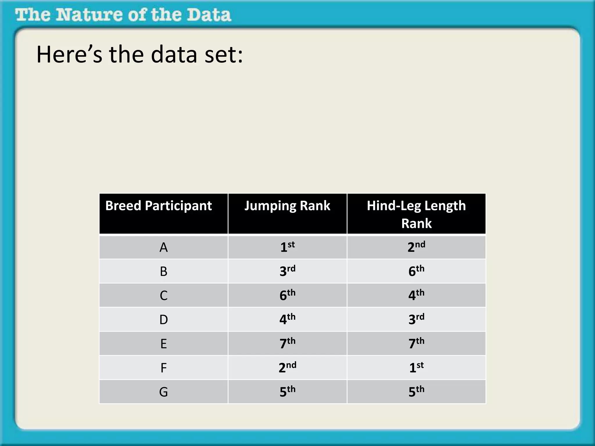
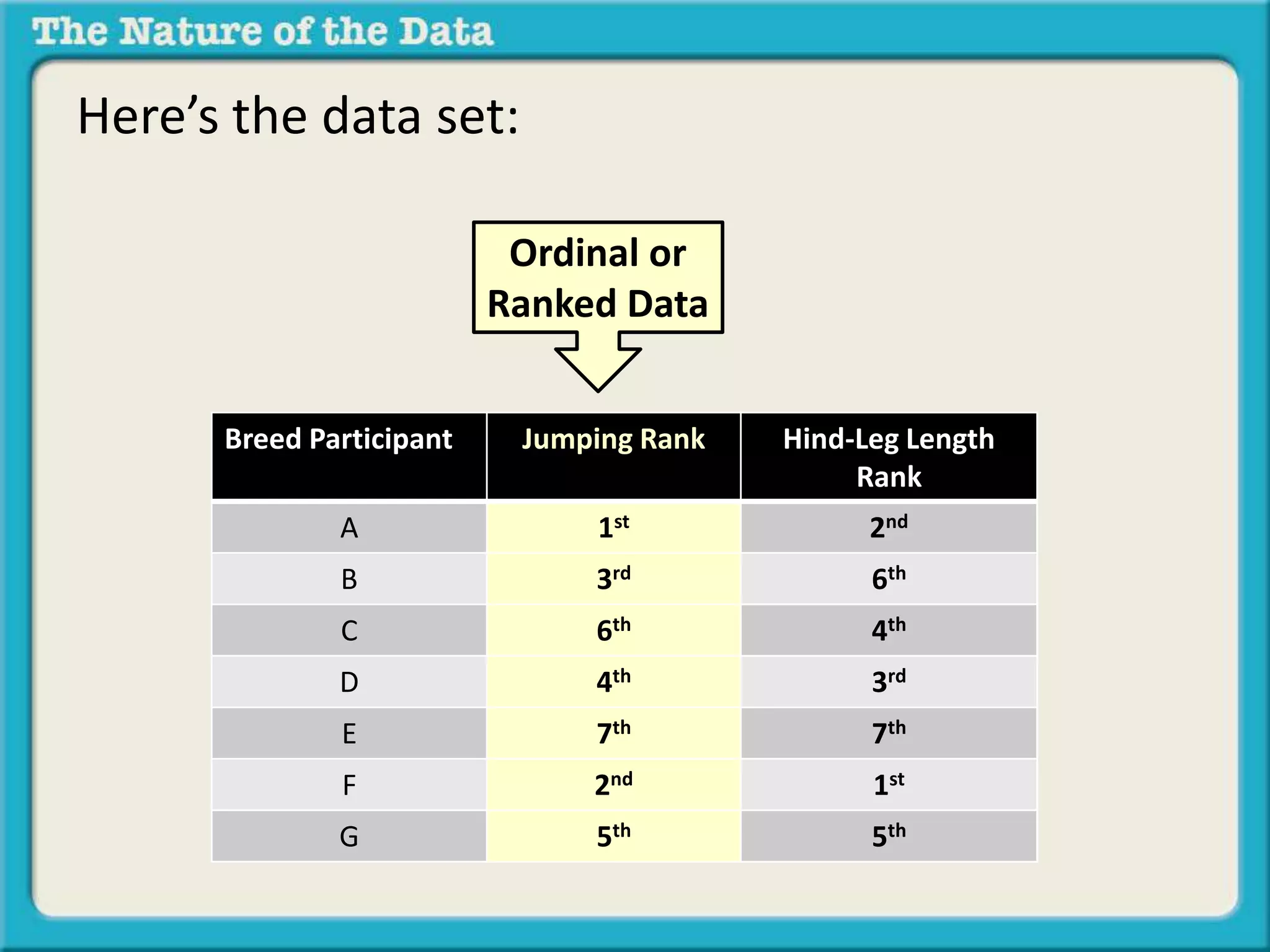
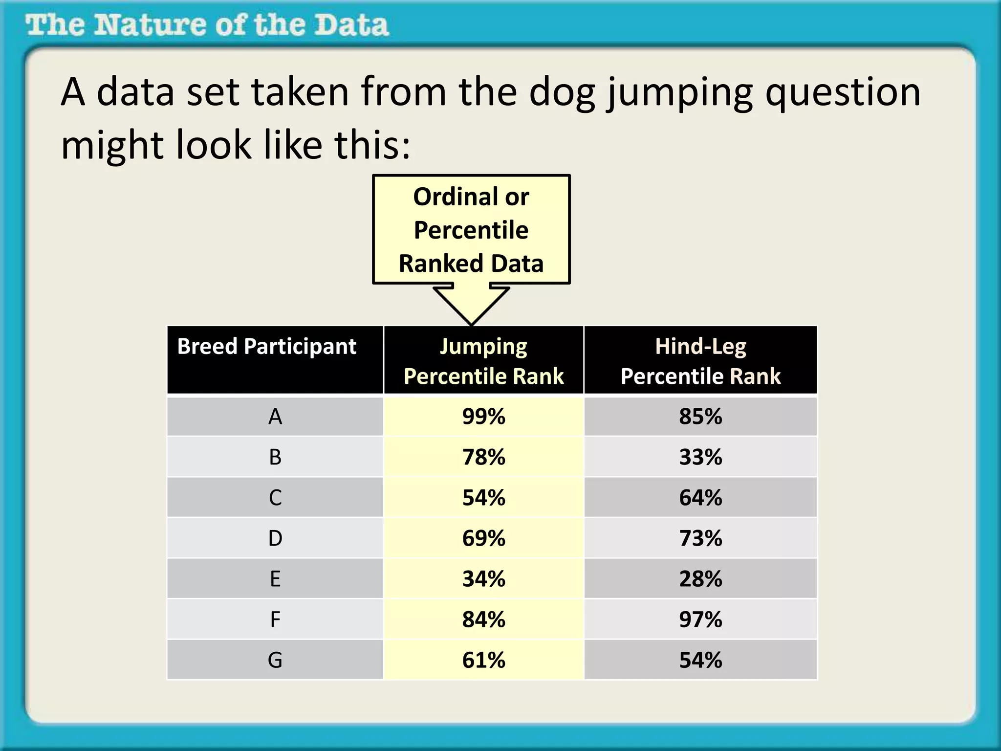
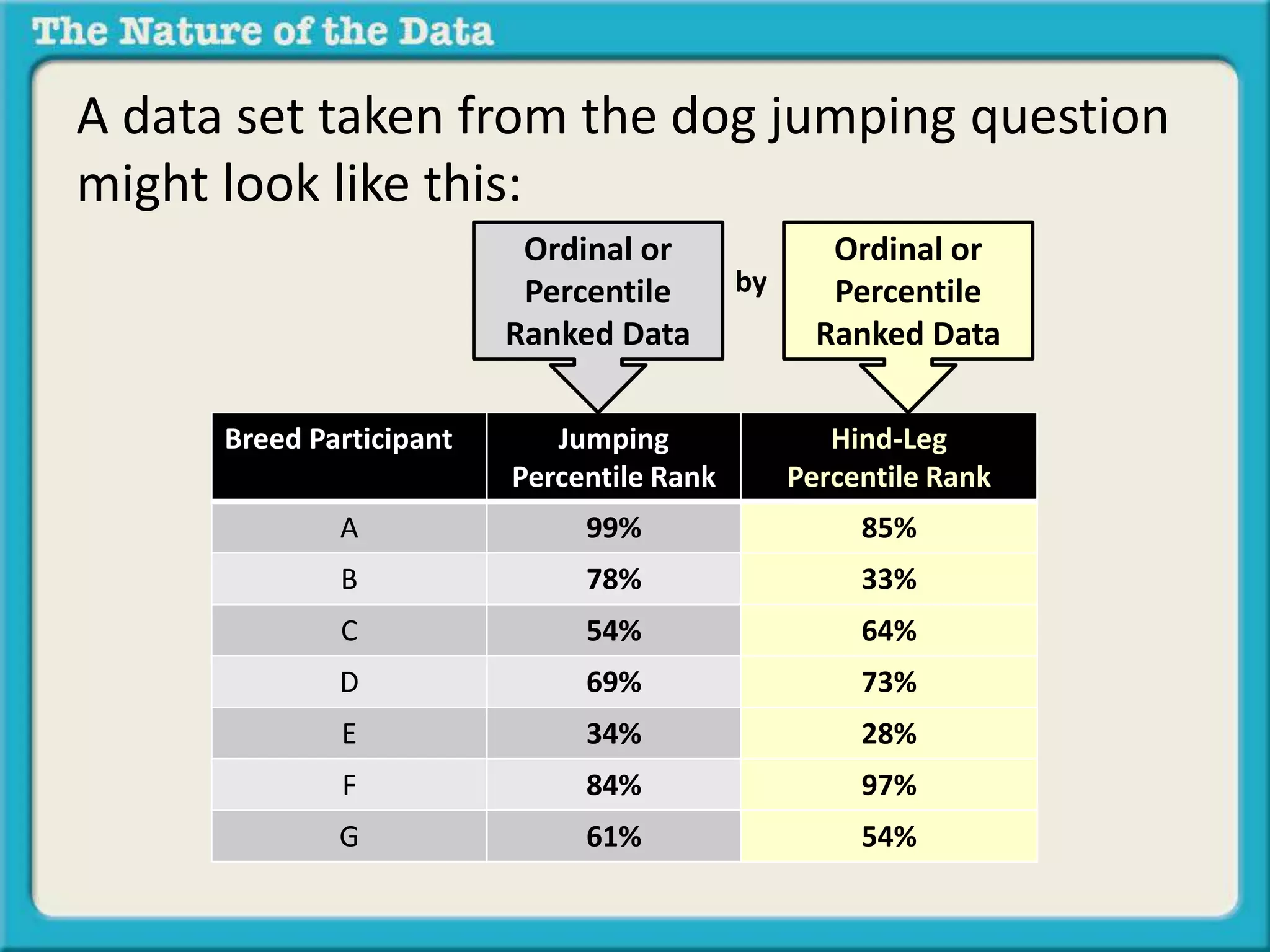
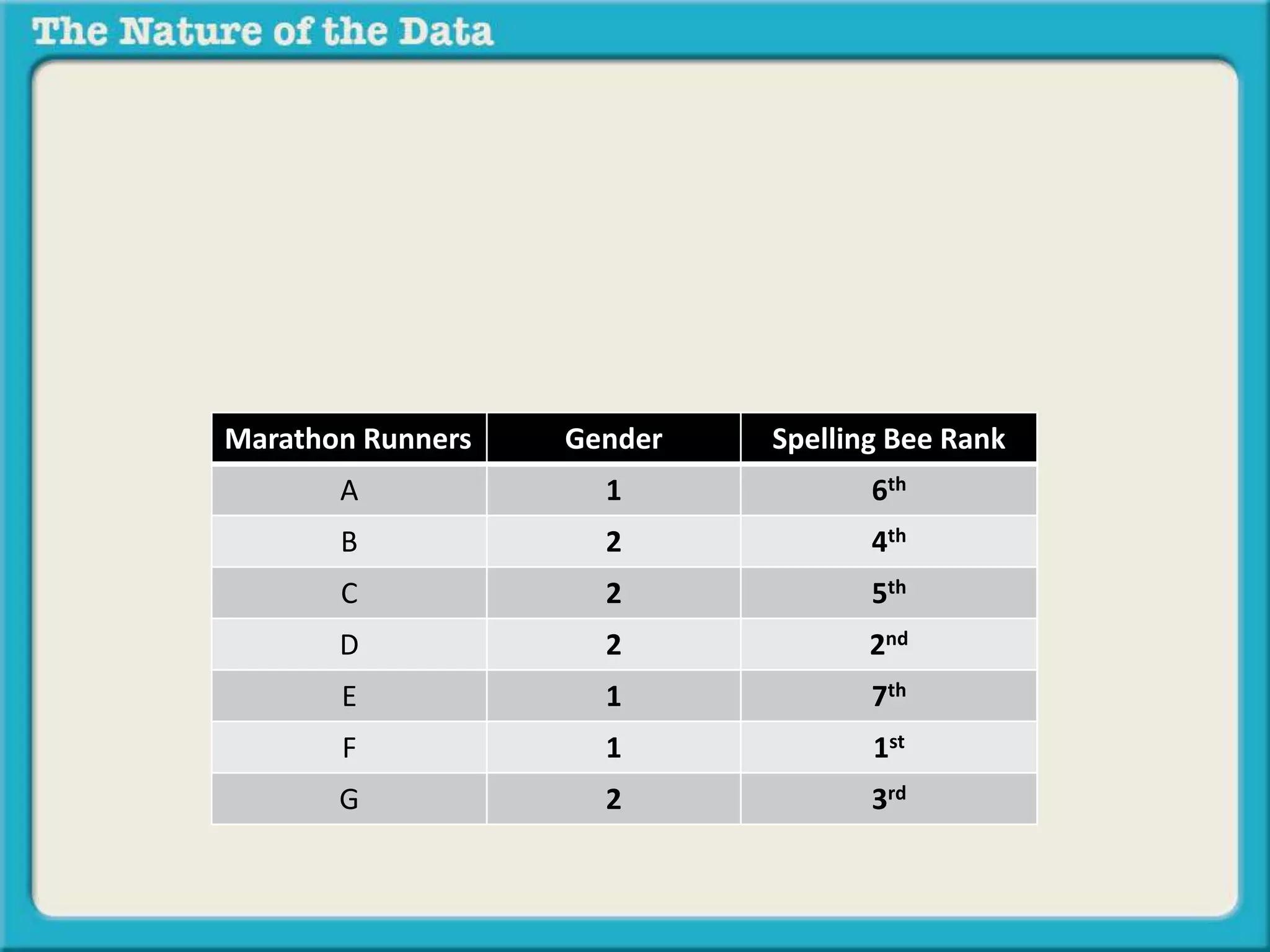
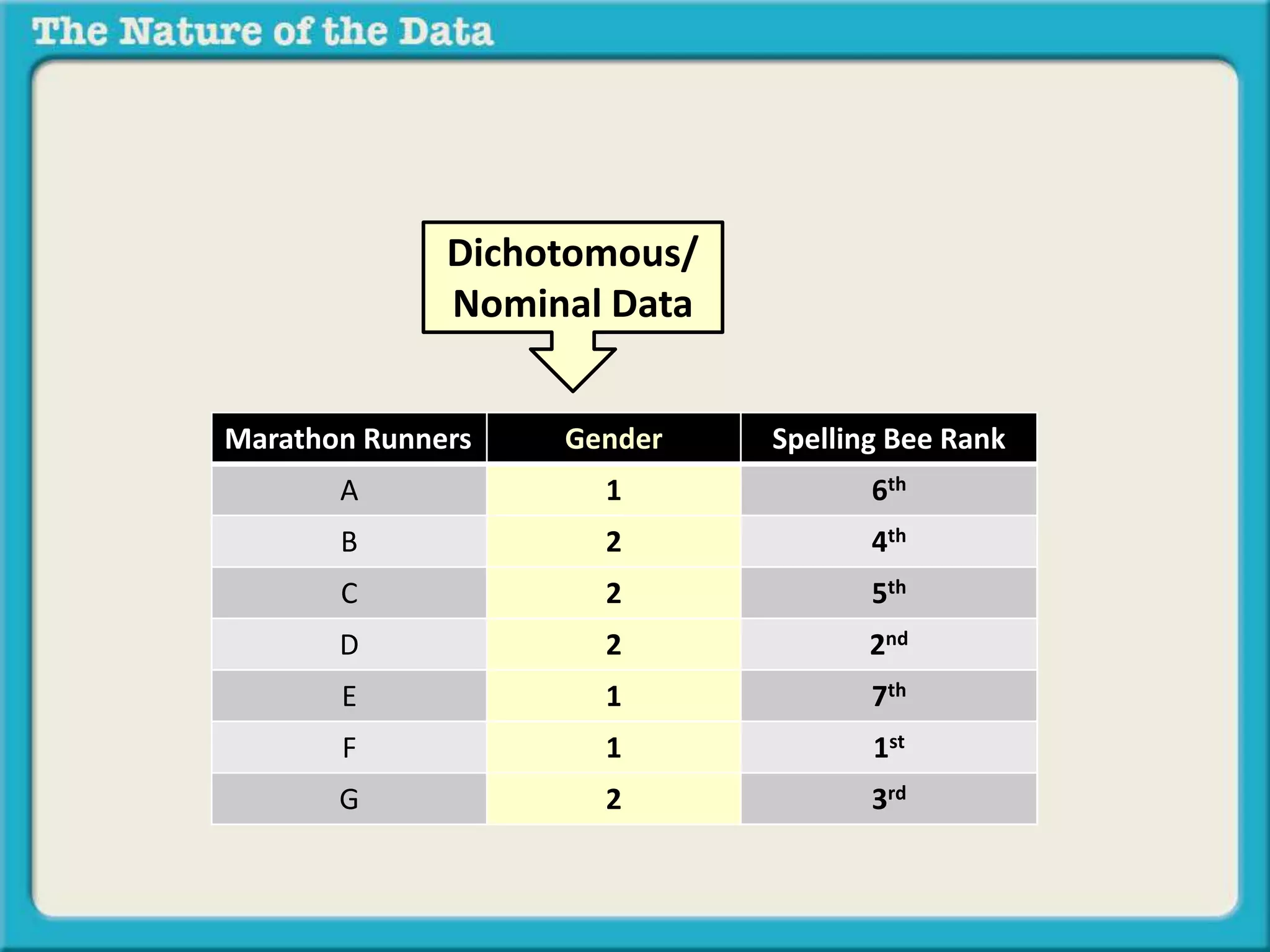
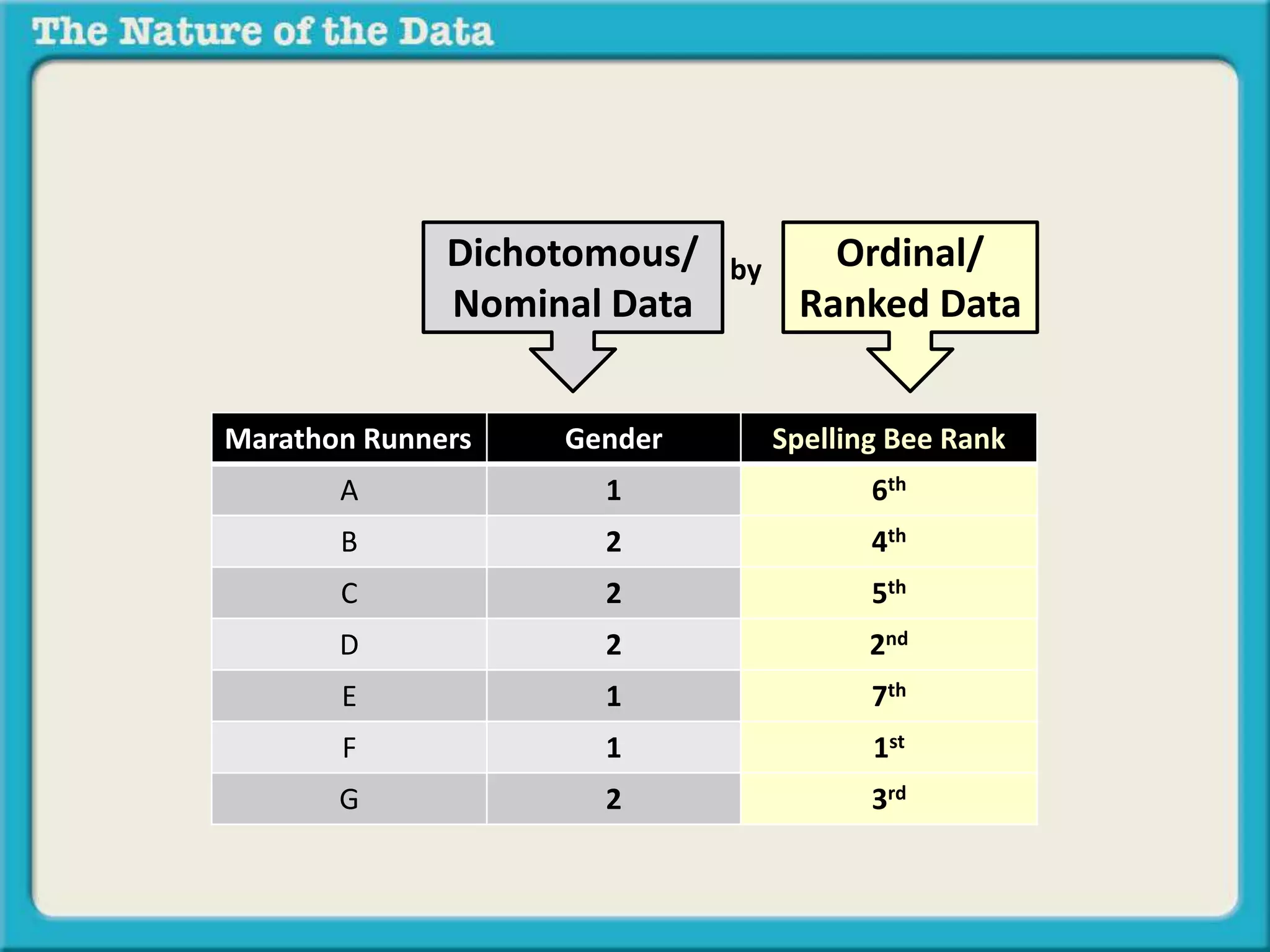
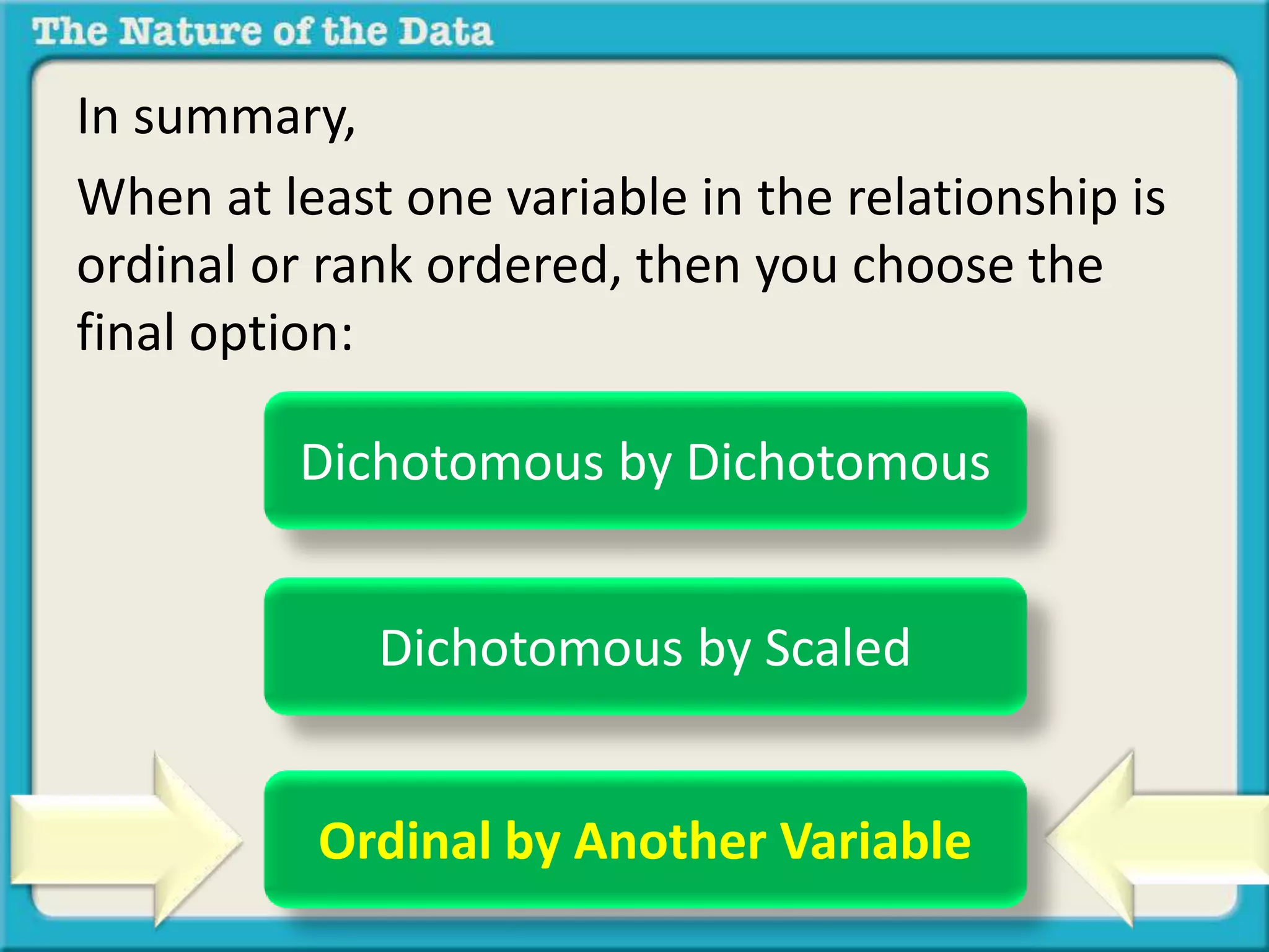
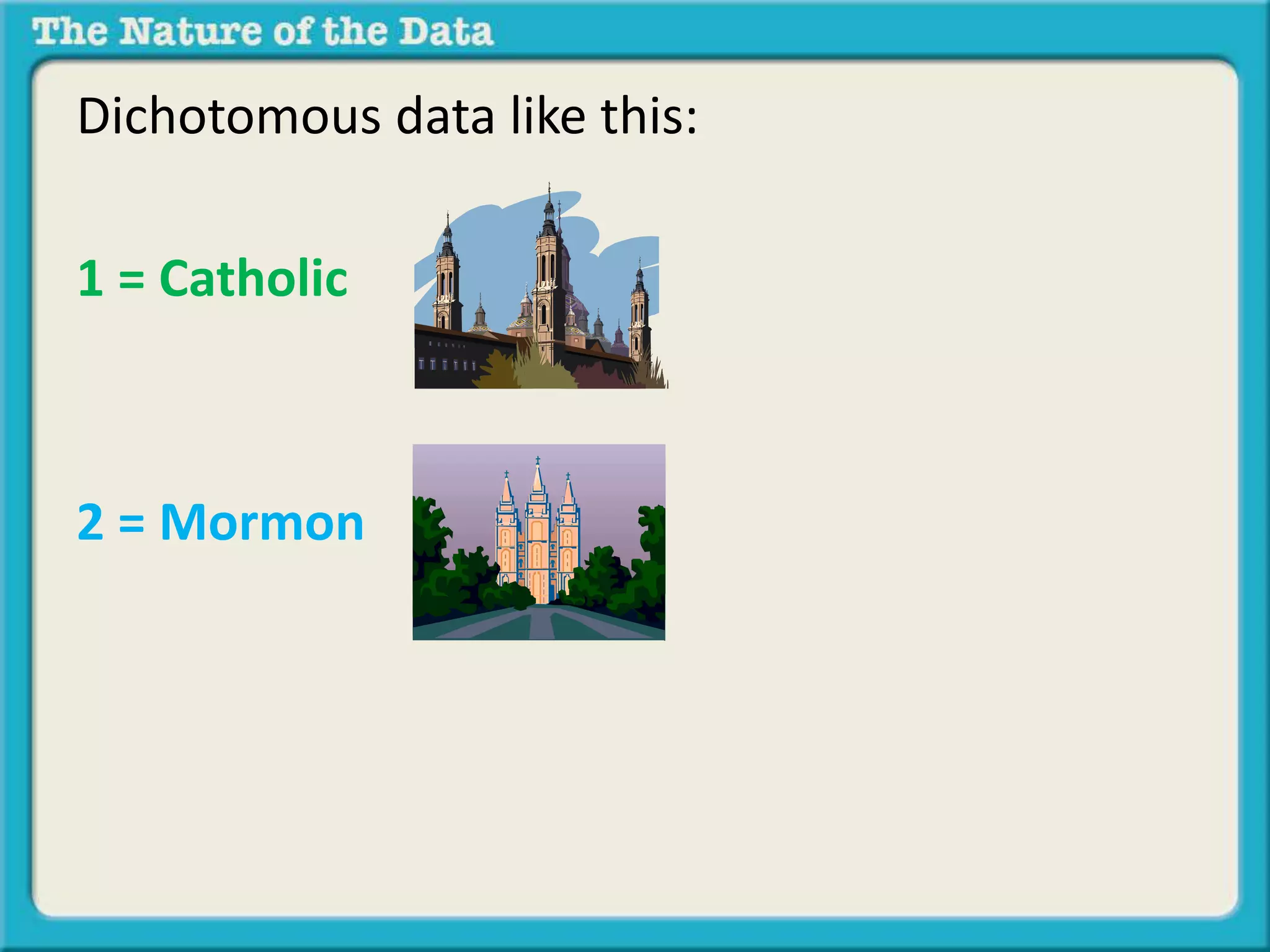
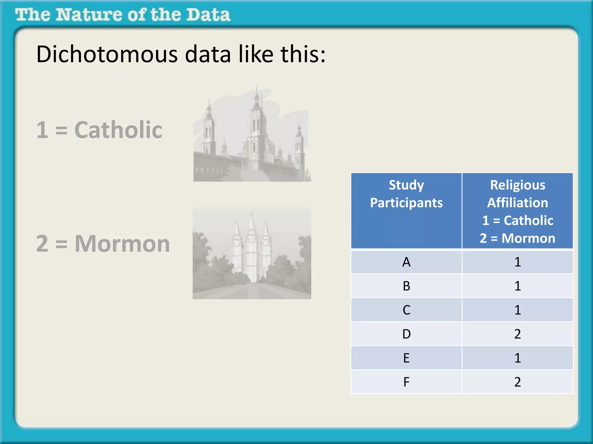
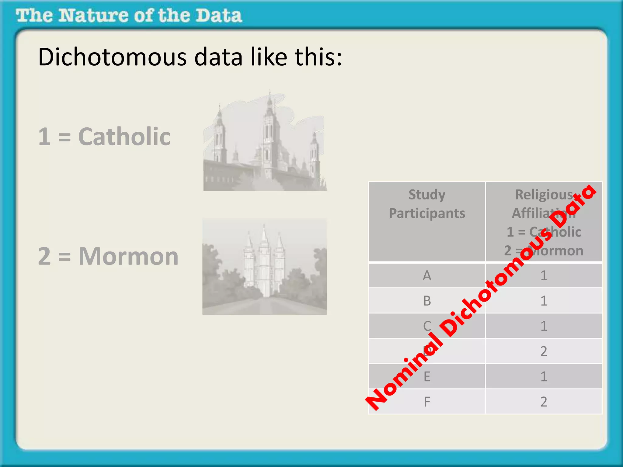
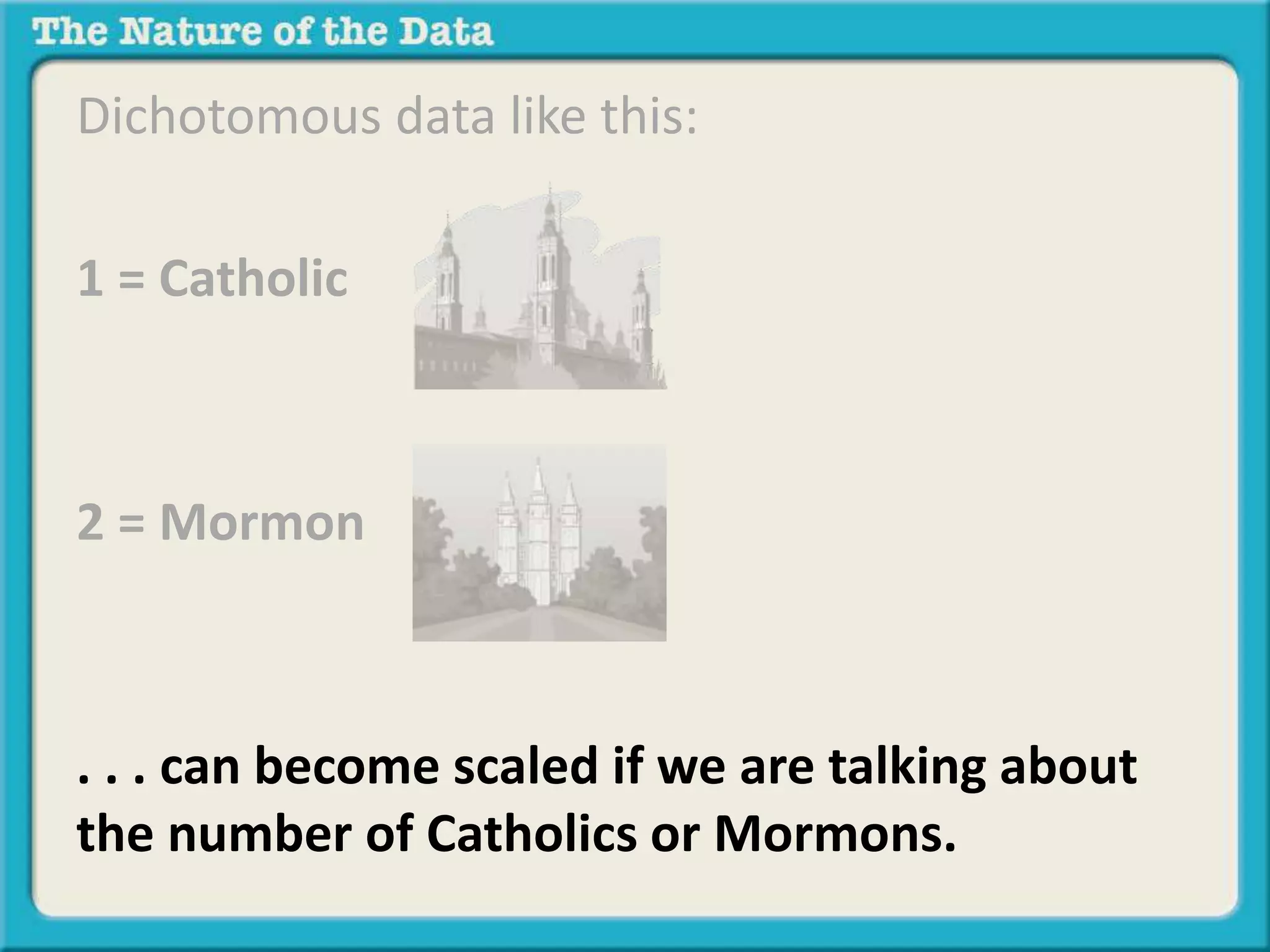
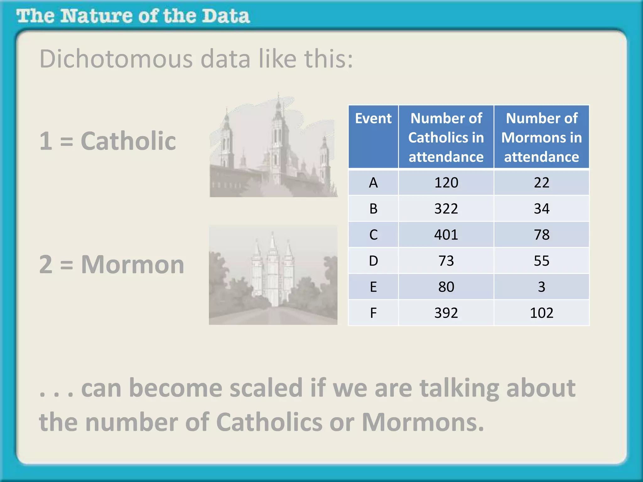
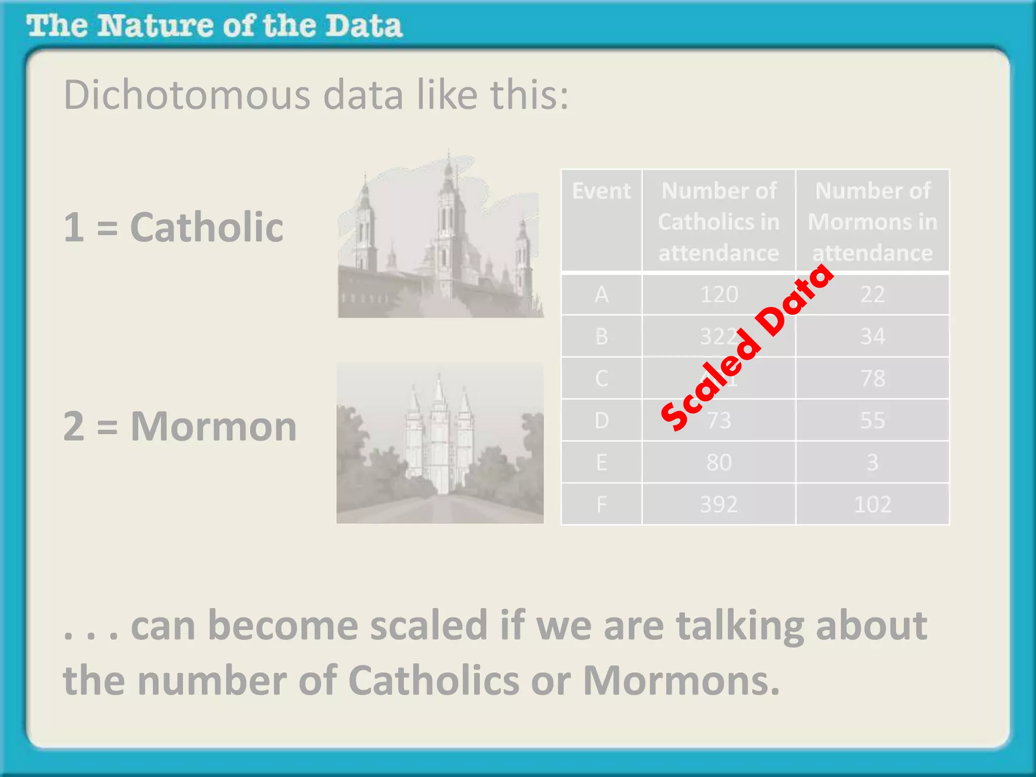
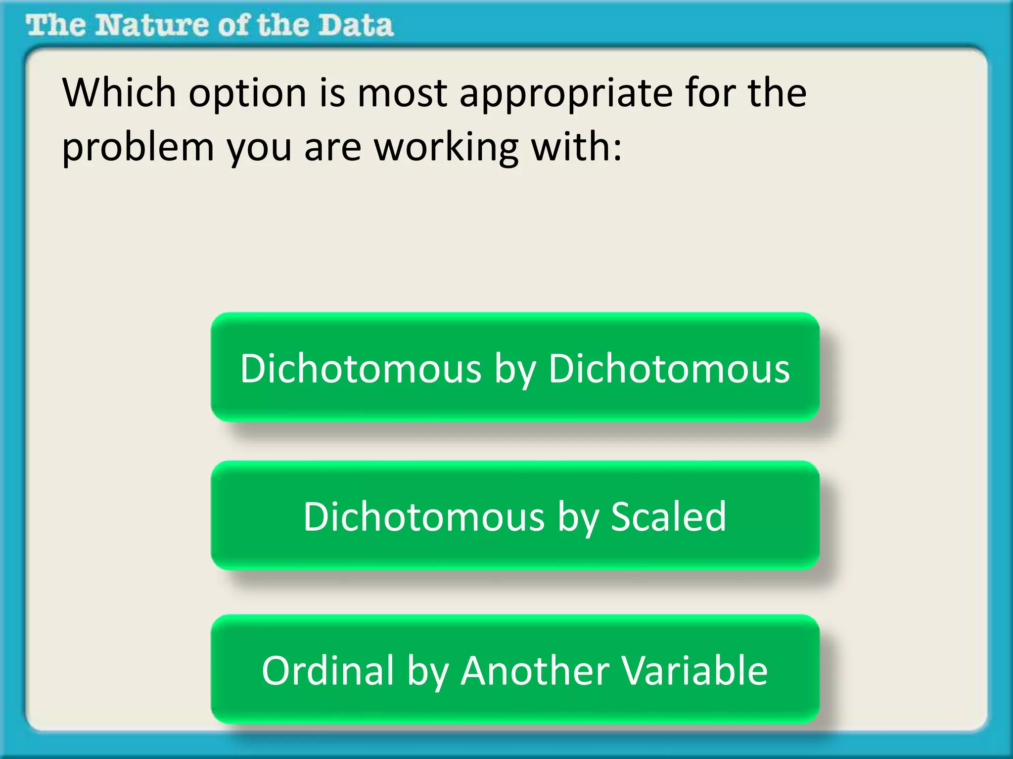
The Nature of Your Data
The purpose of this presentation is to help you 
determine if the two data sets you are working 
with in this problem are:
The purpose of this presentation is to help you 
determine if the two data sets you are working 
with in this problem are: 
Dichotomous by Dichotomous 
Dichotomous by Scaled 
or 
Ordinal by Another Variable
First, let's define 
what each of these mean. 
Dichotomous by Dichotomous 
Dichotomous by Scaled 
or 
Ordinal by Ordinal
Beginning with 
Dichotomous by Dichotomous
What is dichotomous data?
The "Di" in Dichotomous means "two"
. . . and "tomous" or "tomy" as in 
“appendec-tomy” means to divide by.
. . . and "tomous" or "tomy" as in 
“appendec-tomy” means to divide by.
So, dichotomous means to divide by two.
In this case a variable is divided by two or 
specifically it can only take on two values.
For example:
Gender is a good example of a dichotomous 
data.
Gender is a good example of a dichotomous 
data. It generally takes on two values
Gender is a good example of a dichotomous 
data. It generally takes on two values 
(1) male 
(2) female
In some cases individuals are divided by 
(1) those who received a treatment and 
(2) those who did not.
For example:
You have been asked to determine if those who 
eat asparagus score higher on a well-being 
scale (1-10) than those who do not.
You have been asked to determine if those who 
eat asparagus score higher on a well-being 
scale (1-10) than those who do not.
You have been asked to determine if those who 
eat asparagus score higher on a well-being 
scale (1-10) than those who do not. 
In this case, we are dealing with those 
(1) who eat asparagus and those (2) who do not.
With dichotomous by dichotomous data you are 
examining the relationship between two 
dichotomous variables.
Here is an example:
It has been purported that females prefer 
artichokes more than do males.
It has been purported that females prefer 
artichokes more than do males.
It has been purported that females prefer 
artichokes more than do males. 
Dichotomous variable 1: 
Gender 
(1)Male 
(2)Female
It has been purported that females prefer 
artichokes more than do males. 
Dichotomous variable 1: 
Gender 
(1)Male 
(2)Female
It has been purported that females prefer 
artichokes more than do males. 
Dichotomous variable 1: 
Gender 
(1)Male 
(2)Female
It has been purported that females prefer 
artichokes more than do males. 
Dichotomous variable 2: 
Artichoke Preference 
(1)Prefer Artichokes 
(2)Do not prefer Artichokes
It has been purported that females prefer 
artichokes more than do males. 
Dichotomous variable 2: 
Artichoke Preference 
(1)Prefer Artichokes 
(2)Do not prefer Artichokes
It has been purported that females prefer 
artichokes more than do males. 
Dichotomous variable 2: 
Artichoke Preference 
(1)Prefer Artichokes 
(2)Do not prefer Artichokes
Here is what the data set looks like:
It has been purported that females prefer 
artichokes more than do males. 
Study Participant Gender 
1 = Male 
2 = Female 
Artichoke Preference 
1 = Prefer Artichokes 
2 = Don’t Prefer Artichokes 
A 1 2 
B 2 1 
C 1 2 
D 2 1 
E 2 1 
F 1 2 
G 1 2
This is an example of: 
Dichotomous 
Data 
Study Participant Gender 
1 = Male 
2 = Female 
Artichoke Preference 
1 = Prefer Artichokes 
2 = Don’t Prefer Artichokes 
A 1 2 
B 2 1 
C 1 2 
D 2 1 
E 2 1 
F 1 2 
G 1 2
This is an example of: 
Dichotomous 
Data 
Study Participant Gender 
1 = Male 
2 = Female 
by 
Dichotomous 
Data 
Artichoke Preference 
1 = Prefer Artichokes 
2 = Don’t Prefer Artichokes 
A 1 2 
B 2 1 
C 1 2 
D 2 1 
E 2 1 
F 1 2 
G 1 2
As you will learn, there is a specific statistical 
method used to calculate the relationship 
between two dichotomous variables. It is called 
the Phi-coefficient.
Note - a dichotomous variable is also a nominal 
variable.
Note - a dichotomous variable is also a nominal 
variable. However, nominal variables can also 
take on more than two values:
Note - a dichotomous variable is also a nominal 
variable. However, nominal variables can also 
take on more than two values: 
1 = American 
2 = Canadian 
3 = Mexican 
like so
Note - a dichotomous variable is also a nominal 
variable. However, nominal variables can also 
take on more than two values: 
1 = American 
2 = Canadian 
3 = Mexican 
Dichotomous nominal variables can only take on 
two values - (e.g., 1 = Male, 2 = Female)
The next type of relationship involves 
dichotomous by scaled variables.
The next type of relationship involves 
dichotomous by scaled variables. 
Dichotomous by Dichotomous 
Dichotomous by Scaled 
Ordinal by Another Variable
Now you already know what a dichotomous 
variable is, but what is a scaled variable?
A scaled variable is a variable that theoretically 
can take on an infinite amount of values.
A scaled variable is a variable that theoretically 
can take on an infinite amount of values.
For example,
Let's say a car can go as slow as 0 miles per hour 
and as fast as 130 miles per hour.
Within those two points (0 and 130mph) it could 
go 30 mph, 60 mph, 23 mph, 120 mph, 33.2 
mph, 44.302 mph, or even 88.00000000001 
mph.
The point is that between these two points (0 
and 130mph) there are an infinite number of 
values that the speed could take.
Scaled data also has what are called equal 
intervals.
Scaled data also has what are called equal 
intervals. This means that the basic unit of 
measurement (e.g., inches, miles per hour, 
pounds) are the same across the scale:
Scaled data also has what are called equal 
intervals. This means that the basic unit of 
measurement (e.g., inches, miles per hour, 
pounds) are the same across the scale: 
100o - 101o 
70o - 71o 
40o - 41o 
Each set of readings are the same 
distance apart: 1o 
Slide 51
Here is an example of a word problem with 
scaled by dichotomous variables:
You have been asked to determine the 
relationship between age and hours of sleep. 
Age is divided into two groups: Middle Age (45- 
64) and Old Age (65-94).
You have been asked to determine the 
relationship between age and hours of sleep. 
Age is divided into two groups: Middle Age (45- 
64) and Old Age (65-94). 
The Scaled Variable is hours of 
sleep which can take on values 
from 0 to 8+ hours.
You have been asked to determine the 
relationship between age and hours of sleep. 
Age is divided into two groups: Middle Age (45- 
64) and Old Age (65-94). 
The Dichotomous Variable is age 
which in this case can take on two 
values (1) middle and (2) old age.
Here is what the data set might look like:
Here is what the data set might look like: 
Study Participant Age 
1 = 45-64 years 
2 = 65-94 years 
Hours of Sleep 
A 1 6.2 
B 2 9.1 
C 1 5.8 
D 2 8.2 
E 2 7.4 
F 1 4.9 
G 1 6.8
Here is what the data set might look like: 
Dichotomous 
Data 
Study Participant Age 
1 = 45-64 years 
2 = 65-94 years 
Hours of Sleep 
A 1 6.2 
B 2 9.1 
C 1 5.8 
D 2 8.2 
E 2 7.4 
F 1 4.9 
G 1 6.8
Here is what the data set might look like: 
Dichotomous 
Data 
Study Participant Age 
1 = 45-64 years 
2 = 65-94 years 
Hours of Sleep 
A 1 6.2 
B 2 9.1 
C 1 5.8 
D 2 8.2 
E 2 7.4 
F 1 4.9 
G 1 6.8
Here is what the data set might look like: 
Dichotomous 
Data 
Study Participant Age 
1 = 45-64 years 
2 = 65-94 years 
Hours of Sleep 
by 
A 1 6.2 
B 2 9.1 
C 1 5.8 
D 2 8.2 
E 2 7.4 
F 1 4.9 
G 1 6.8
Here is what the data set might look like: 
Dichotomous 
Data 
Study Participant Age 
1 = 45-64 years 
2 = 65-94 years 
Scaled 
Data 
Hours of Sleep 
by 
A 1 6.2 
B 2 9.1 
C 1 5.8 
D 2 8.2 
E 2 7.4 
F 1 4.9 
G 1 6.8
Note, in the strictest sense scaled data should 
be like the car example (values are infinite 
between 0 and 130 mph).
However, in the social sciences many times data 
that is technically not scaled (e.g., on a scale of 
1-10 how would you rate the ballerina's 
performance), are still treated as scaled data.
However, in the social sciences many times data 
that is technically not scaled (e.g., on a scale of 
1-10 how would you rate the ballerina's 
performance), are still treated as scaled data. 
Yes, it is true there are only 10 values that the 
variable can take on, but many researchers will 
treat it as scaled data. For the purposes of this 
class we will treat variables such as these as 
scaled data as well.
However, if we were rating on a scale of 1-2, 1-3 
or 1-4 we most likely would not treat such 
variables as scaled.
As you will learn there is a specific statistical 
method used to calculate the relationship 
between scaled by dichotomous variables. it is 
called the Point Biserial Correlation.
Lastly let's consider the relationship involving 
ordinal data by another variable.
Lastly let's consider the relationship involving 
ordinal data by another variable. 
Dichotomous by Dichotomous 
Dichotomous by Scaled 
Ordinal by Another Variable
An ordinal variable is a variable where the 
numbers represent relative amounts of a an 
attribute. However, they do not have equal 
intervals.
For example,
In this pole vaulting example you will notice that 
1st and 2nd place are closer to each other:
In this pole vaulting example you will notice that 
1st and 2nd place are closer to each other: 
3rd 
Place 
15’ 2” 
2nd 
Place 
18’ 1” 
1st 
Place 
18’ 3”
In this pole vaulting example you will notice that 
1st and 2nd place are closer to each other: 
3rd 
Place 
15’ 2” 
2nd 
Place 
18’ 1” 
1st 
Place 
18’ 3”
In this pole vaulting example you will notice that 
1st and 2nd place are closer to each other: 
3rd 
Place 
15’ 2” 
2nd 
Place 
18’ 1” 
1st 
Place 
18’ 3” 
2 inches 
apart
. . . than 2nd and 3rd place, which are much 
further apart
. . . than 2nd and 3rd place, which are much 
further apart 
3rd 
Place 
15’ 2” 
2nd 
Place 
18’ 1” 
1st 
Place 
18’ 3”
. . . than 2nd and 3rd place, which are much 
further apart 
3rd 
Place 
15’ 2” 
2nd 
Place 
18’ 1” 
1st 
Place 
18’ 3” 
3 feet 
1” apart
Rank ordered or ordinal data such as these do 
not have equal intervals. 
3rd 
Place 
15’ 2” 
2nd 
Place 
18’ 1” 
1st 
Place 
18’ 3”
Rank ordered or ordinal data such as these do 
not have equal intervals. 
3rd 
Place 
15’ 2” 
2nd 
Place 
18’ 1” 
1st 
Place 
18’ 3”
Here is what an ordinal by ordinal problem looks 
like:
In a study, researchers rank order different 
breeds of dog based on how high they can jump. 
They then rank order them based on the length 
of their hind legs. They wish to determine if a 
relationship exists between jumping height and 
hind leg length.
In a study, researchers rank order different 
breeds of dog based on how high they can jump. 
They then rank order them based on the length 
of their hind legs. They wish to determine if a 
relationship exists between jumping height and 
hind leg length.
In a study, researchers rank order different 
breeds of dog based on how high they can jump. 
They then rank order them based on the length 
of their hind legs. They wish to determine if a 
relationship exists between jumping height and 
hind leg length.
Here’s the data set:
Here’s the data set: 
Breed Participant Jumping Rank Hind-Leg Length 
Rank 
A 1st 2nd 
B 3rd 6th 
C 6th 4th 
D 4th 3rd 
E 7th 7th 
F 2nd 1st 
G 5th 5th
Here’s the data set: 
Ordinal or 
Ranked Data 
Breed Participant Jumping Rank Hind-Leg Length 
Rank 
A 1st 2nd 
B 3rd 6th 
C 6th 4th 
D 4th 3rd 
E 7th 7th 
F 2nd 1st 
G 5th 5th
Here’s the data set: 
by 
Ordinal or 
Ranked Data 
Ordinal or 
Ranked Data 
Breed Participant Jumping Rank Hind-Leg Length 
Rank 
A 1st 2nd 
B 3rd 6th 
C 6th 4th 
D 4th 3rd 
E 7th 7th 
F 2nd 1st 
G 5th 5th
Rank ordered data can also take the form of 
percentiles.
Percentiles communicate the percentage of 
observations or values below a certain point.
If my score on the ACT is at the 35th percentile 
that means the 35% of ACT takers are below me.
If my score on the ACT is at the 35th percentile 
that means the 35% of ACT takers are below me.
A data set taken from the dog jumping question 
might look like this:
A data set taken from the dog jumping question 
might look like this: 
Breed Participant Jumping 
Percentile Rank 
Hind-Leg 
Percentile Rank 
A 99% 85% 
B 78% 33% 
C 54% 64% 
D 69% 73% 
E 34% 28% 
F 84% 97% 
G 61% 54%
A data set taken from the dog jumping question 
might look like this: 
Ordinal or 
Percentile 
Ranked Data 
Breed Participant Jumping 
Percentile Rank 
Hind-Leg 
Percentile Rank 
A 99% 85% 
B 78% 33% 
C 54% 64% 
D 69% 73% 
E 34% 28% 
F 84% 97% 
G 61% 54%
A data set taken from the dog jumping question 
might look like this: 
Ordinal or 
Percentile 
Ranked Data 
Breed Participant Jumping 
Percentile Rank 
Ordinal or 
Percentile 
Ranked Data 
Hind-Leg 
Percentile Rank 
by 
A 99% 85% 
B 78% 33% 
C 54% 64% 
D 69% 73% 
E 34% 28% 
F 84% 97% 
G 61% 54%
The next example is that of a relationship 
between ordinal variable and a scaled variable.
You have been asked to determine if there is a 
relationship between the height of marathon 
runners and their final ranking in a race.
You have been asked to determine if there is a 
relationship between the height of marathon 
runners and their final ranking in a race.
Here’s the data set: 
Marathon Runners Height in inches Order of Finish 
A 73 6th 
B 67 4th 
C 69 5th 
D 64 2nd 
E 71 7th 
F 62 1st 
G 66 3rd
Here’s the data set: 
Scaled 
Data 
Marathon Runners Height in inches Order of Finish 
A 73 6th 
B 67 4th 
C 69 5th 
D 64 2nd 
E 71 7th 
F 62 1st 
G 66 3rd
Here’s the data set: 
Scaled 
Data 
by Ordinal/ 
Ranked Data 
Marathon Runners Height in inches Order of Finish 
A 73 6th 
B 67 4th 
C 69 5th 
D 64 2nd 
E 71 7th 
F 62 1st 
G 66 3rd
The final example is that of a relationship 
between ordinal variable and a nominal 
variable.
You have been asked to determine if there is a 
relationship between gender and spelling bee 
competition rankings.
You have been asked to determine if there is a 
relationship between gender and spelling bee 
competition rankings.
Here’s the data set:
Marathon Runners Gender Spelling Bee Rank 
A 1 6th 
B 2 4th 
C 2 5th 
D 2 2nd 
E 1 7th 
F 1 1st 
G 2 3rd
Dichotomous/ 
Nominal Data 
Marathon Runners Gender Spelling Bee Rank 
A 1 6th 
B 2 4th 
C 2 5th 
D 2 2nd 
E 1 7th 
F 1 1st 
G 2 3rd
by Ordinal/ 
Ranked Data 
Dichotomous/ 
Nominal Data 
Marathon Runners Gender Spelling Bee Rank 
A 1 6th 
B 2 4th 
C 2 5th 
D 2 2nd 
E 1 7th 
F 1 1st 
G 2 3rd
In summary,
In summary, 
When at least one variable in the relationship is 
ordinal or rank ordered, then you choose the 
final option:
In summary, 
When at least one variable in the relationship is 
ordinal or rank ordered, then you choose the 
final option: 
Dichotomous by Dichotomous 
Dichotomous by Scaled 
Ordinal by Another Variable
As you will learn there are specific statistical 
methods used to calculate the relationship 
between ordinal by ordinal or ordinal by other 
variables.
As you will learn there are specific statistical 
methods used to calculate the relationship 
between ordinal by ordinal or ordinal by other 
variables. They are the Spearman Rho and 
Kendall Tau.
As you will learn there are specific statistical 
methods used to calculate the relationship 
between ordinal by ordinal or ordinal by other 
variables. They are the Spearman Rho and 
Kendall Tau. We'll explain their difference in 
another presentation.
A final note:
Dichotomous data like this: 
1 = Catholic 
2 = Mormon
Dichotomous data like this: 
1 = Catholic 
2 = Mormon 
Study 
Participants 
Religious 
Affiliation 
1 = Catholic 
2 = Mormon 
A 1 
B 1 
C 1 
D 2 
E 1 
F 2
Dichotomous data like this: 
1 = Catholic 
2 = Mormon 
Study 
Participants 
Religious 
Affiliation 
1 = Catholic 
2 = Mormon 
A 1 
B 1 
C 1 
D 2 
E 1 
F 2
Dichotomous data like this: 
1 = Catholic 
2 = Mormon 
. . . can become scaled if we are talking about 
the number of Catholics or Mormons.
Dichotomous data like this: 
1 = Catholic 
2 = Mormon 
Event Number of 
Catholics in 
attendance 
Number of 
Mormons in 
attendance 
A 120 22 
B 322 34 
C 401 78 
D 73 55 
E 80 3 
F 392 102 
. . . can become scaled if we are talking about 
the number of Catholics or Mormons.
Dichotomous data like this: 
1 = Catholic 
2 = Mormon 
Event Number of 
Catholics in 
attendance 
Number of 
Mormons in 
attendance 
A 120 22 
B 322 34 
C 401 78 
D 73 55 
E 80 3 
F 392 102 
. . . can become scaled if we are talking about 
the number of Catholics or Mormons.
Which option is most appropriate for the 
problem you are working with: 
Dichotomous by Dichotomous 
Dichotomous by Scaled 
Ordinal by Another Variable

The nature of the data

  • 1.
    The Nature ofYour Data
  • 2.
    The purpose ofthis presentation is to help you determine if the two data sets you are working with in this problem are:
  • 3.
    The purpose ofthis presentation is to help you determine if the two data sets you are working with in this problem are: Dichotomous by Dichotomous Dichotomous by Scaled or Ordinal by Another Variable
  • 4.
    First, let's define what each of these mean. Dichotomous by Dichotomous Dichotomous by Scaled or Ordinal by Ordinal
  • 5.
  • 6.
  • 7.
    The "Di" inDichotomous means "two"
  • 8.
    . . .and "tomous" or "tomy" as in “appendec-tomy” means to divide by.
  • 9.
    . . .and "tomous" or "tomy" as in “appendec-tomy” means to divide by.
  • 10.
    So, dichotomous meansto divide by two.
  • 11.
    In this casea variable is divided by two or specifically it can only take on two values.
  • 12.
  • 13.
    Gender is agood example of a dichotomous data.
  • 14.
    Gender is agood example of a dichotomous data. It generally takes on two values
  • 15.
    Gender is agood example of a dichotomous data. It generally takes on two values (1) male (2) female
  • 16.
    In some casesindividuals are divided by (1) those who received a treatment and (2) those who did not.
  • 17.
  • 18.
    You have beenasked to determine if those who eat asparagus score higher on a well-being scale (1-10) than those who do not.
  • 19.
    You have beenasked to determine if those who eat asparagus score higher on a well-being scale (1-10) than those who do not.
  • 20.
    You have beenasked to determine if those who eat asparagus score higher on a well-being scale (1-10) than those who do not. In this case, we are dealing with those (1) who eat asparagus and those (2) who do not.
  • 21.
    With dichotomous bydichotomous data you are examining the relationship between two dichotomous variables.
  • 22.
    Here is anexample:
  • 23.
    It has beenpurported that females prefer artichokes more than do males.
  • 24.
    It has beenpurported that females prefer artichokes more than do males.
  • 25.
    It has beenpurported that females prefer artichokes more than do males. Dichotomous variable 1: Gender (1)Male (2)Female
  • 26.
    It has beenpurported that females prefer artichokes more than do males. Dichotomous variable 1: Gender (1)Male (2)Female
  • 27.
    It has beenpurported that females prefer artichokes more than do males. Dichotomous variable 1: Gender (1)Male (2)Female
  • 28.
    It has beenpurported that females prefer artichokes more than do males. Dichotomous variable 2: Artichoke Preference (1)Prefer Artichokes (2)Do not prefer Artichokes
  • 29.
    It has beenpurported that females prefer artichokes more than do males. Dichotomous variable 2: Artichoke Preference (1)Prefer Artichokes (2)Do not prefer Artichokes
  • 30.
    It has beenpurported that females prefer artichokes more than do males. Dichotomous variable 2: Artichoke Preference (1)Prefer Artichokes (2)Do not prefer Artichokes
  • 31.
    Here is whatthe data set looks like:
  • 32.
    It has beenpurported that females prefer artichokes more than do males. Study Participant Gender 1 = Male 2 = Female Artichoke Preference 1 = Prefer Artichokes 2 = Don’t Prefer Artichokes A 1 2 B 2 1 C 1 2 D 2 1 E 2 1 F 1 2 G 1 2
  • 33.
    This is anexample of: Dichotomous Data Study Participant Gender 1 = Male 2 = Female Artichoke Preference 1 = Prefer Artichokes 2 = Don’t Prefer Artichokes A 1 2 B 2 1 C 1 2 D 2 1 E 2 1 F 1 2 G 1 2
  • 34.
    This is anexample of: Dichotomous Data Study Participant Gender 1 = Male 2 = Female by Dichotomous Data Artichoke Preference 1 = Prefer Artichokes 2 = Don’t Prefer Artichokes A 1 2 B 2 1 C 1 2 D 2 1 E 2 1 F 1 2 G 1 2
  • 35.
    As you willlearn, there is a specific statistical method used to calculate the relationship between two dichotomous variables. It is called the Phi-coefficient.
  • 36.
    Note - adichotomous variable is also a nominal variable.
  • 37.
    Note - adichotomous variable is also a nominal variable. However, nominal variables can also take on more than two values:
  • 38.
    Note - adichotomous variable is also a nominal variable. However, nominal variables can also take on more than two values: 1 = American 2 = Canadian 3 = Mexican like so
  • 39.
    Note - adichotomous variable is also a nominal variable. However, nominal variables can also take on more than two values: 1 = American 2 = Canadian 3 = Mexican Dichotomous nominal variables can only take on two values - (e.g., 1 = Male, 2 = Female)
  • 40.
    The next typeof relationship involves dichotomous by scaled variables.
  • 41.
    The next typeof relationship involves dichotomous by scaled variables. Dichotomous by Dichotomous Dichotomous by Scaled Ordinal by Another Variable
  • 42.
    Now you alreadyknow what a dichotomous variable is, but what is a scaled variable?
  • 43.
    A scaled variableis a variable that theoretically can take on an infinite amount of values.
  • 44.
    A scaled variableis a variable that theoretically can take on an infinite amount of values.
  • 45.
  • 46.
    Let's say acar can go as slow as 0 miles per hour and as fast as 130 miles per hour.
  • 47.
    Within those twopoints (0 and 130mph) it could go 30 mph, 60 mph, 23 mph, 120 mph, 33.2 mph, 44.302 mph, or even 88.00000000001 mph.
  • 48.
    The point isthat between these two points (0 and 130mph) there are an infinite number of values that the speed could take.
  • 49.
    Scaled data alsohas what are called equal intervals.
  • 50.
    Scaled data alsohas what are called equal intervals. This means that the basic unit of measurement (e.g., inches, miles per hour, pounds) are the same across the scale:
  • 51.
    Scaled data alsohas what are called equal intervals. This means that the basic unit of measurement (e.g., inches, miles per hour, pounds) are the same across the scale: 100o - 101o 70o - 71o 40o - 41o Each set of readings are the same distance apart: 1o Slide 51
  • 52.
    Here is anexample of a word problem with scaled by dichotomous variables:
  • 53.
    You have beenasked to determine the relationship between age and hours of sleep. Age is divided into two groups: Middle Age (45- 64) and Old Age (65-94).
  • 54.
    You have beenasked to determine the relationship between age and hours of sleep. Age is divided into two groups: Middle Age (45- 64) and Old Age (65-94). The Scaled Variable is hours of sleep which can take on values from 0 to 8+ hours.
  • 55.
    You have beenasked to determine the relationship between age and hours of sleep. Age is divided into two groups: Middle Age (45- 64) and Old Age (65-94). The Dichotomous Variable is age which in this case can take on two values (1) middle and (2) old age.
  • 56.
    Here is whatthe data set might look like:
  • 57.
    Here is whatthe data set might look like: Study Participant Age 1 = 45-64 years 2 = 65-94 years Hours of Sleep A 1 6.2 B 2 9.1 C 1 5.8 D 2 8.2 E 2 7.4 F 1 4.9 G 1 6.8
  • 58.
    Here is whatthe data set might look like: Dichotomous Data Study Participant Age 1 = 45-64 years 2 = 65-94 years Hours of Sleep A 1 6.2 B 2 9.1 C 1 5.8 D 2 8.2 E 2 7.4 F 1 4.9 G 1 6.8
  • 59.
    Here is whatthe data set might look like: Dichotomous Data Study Participant Age 1 = 45-64 years 2 = 65-94 years Hours of Sleep A 1 6.2 B 2 9.1 C 1 5.8 D 2 8.2 E 2 7.4 F 1 4.9 G 1 6.8
  • 60.
    Here is whatthe data set might look like: Dichotomous Data Study Participant Age 1 = 45-64 years 2 = 65-94 years Hours of Sleep by A 1 6.2 B 2 9.1 C 1 5.8 D 2 8.2 E 2 7.4 F 1 4.9 G 1 6.8
  • 61.
    Here is whatthe data set might look like: Dichotomous Data Study Participant Age 1 = 45-64 years 2 = 65-94 years Scaled Data Hours of Sleep by A 1 6.2 B 2 9.1 C 1 5.8 D 2 8.2 E 2 7.4 F 1 4.9 G 1 6.8
  • 62.
    Note, in thestrictest sense scaled data should be like the car example (values are infinite between 0 and 130 mph).
  • 63.
    However, in thesocial sciences many times data that is technically not scaled (e.g., on a scale of 1-10 how would you rate the ballerina's performance), are still treated as scaled data.
  • 64.
    However, in thesocial sciences many times data that is technically not scaled (e.g., on a scale of 1-10 how would you rate the ballerina's performance), are still treated as scaled data. Yes, it is true there are only 10 values that the variable can take on, but many researchers will treat it as scaled data. For the purposes of this class we will treat variables such as these as scaled data as well.
  • 65.
    However, in thesocial sciences many times data that is technically not scaled (e.g., on a scale of 1-10 how would you rate the ballerina's performance), are still treated as scaled data. Yes, it is true there are only 10 values that the variable can take on, but many researchers will treat it as scaled data. For the purposes of this class we will treat variables such as these as scaled data as well.
  • 66.
    However, if wewere rating on a scale of 1-2, 1-3 or 1-4 we most likely would not treat such variables as scaled.
  • 67.
    As you willlearn there is a specific statistical method used to calculate the relationship between scaled by dichotomous variables. it is called the Point Biserial Correlation.
  • 68.
    Lastly let's considerthe relationship involving ordinal data by another variable.
  • 69.
    Lastly let's considerthe relationship involving ordinal data by another variable. Dichotomous by Dichotomous Dichotomous by Scaled Ordinal by Another Variable
  • 70.
    An ordinal variableis a variable where the numbers represent relative amounts of a an attribute. However, they do not have equal intervals.
  • 71.
  • 72.
    In this polevaulting example you will notice that 1st and 2nd place are closer to each other:
  • 73.
    In this polevaulting example you will notice that 1st and 2nd place are closer to each other: 3rd Place 15’ 2” 2nd Place 18’ 1” 1st Place 18’ 3”
  • 74.
    In this polevaulting example you will notice that 1st and 2nd place are closer to each other: 3rd Place 15’ 2” 2nd Place 18’ 1” 1st Place 18’ 3”
  • 75.
    In this polevaulting example you will notice that 1st and 2nd place are closer to each other: 3rd Place 15’ 2” 2nd Place 18’ 1” 1st Place 18’ 3” 2 inches apart
  • 76.
    . . .than 2nd and 3rd place, which are much further apart
  • 77.
    . . .than 2nd and 3rd place, which are much further apart 3rd Place 15’ 2” 2nd Place 18’ 1” 1st Place 18’ 3”
  • 78.
    . . .than 2nd and 3rd place, which are much further apart 3rd Place 15’ 2” 2nd Place 18’ 1” 1st Place 18’ 3” 3 feet 1” apart
  • 79.
    Rank ordered orordinal data such as these do not have equal intervals. 3rd Place 15’ 2” 2nd Place 18’ 1” 1st Place 18’ 3”
  • 80.
    Rank ordered orordinal data such as these do not have equal intervals. 3rd Place 15’ 2” 2nd Place 18’ 1” 1st Place 18’ 3”
  • 81.
    Here is whatan ordinal by ordinal problem looks like:
  • 82.
    In a study,researchers rank order different breeds of dog based on how high they can jump. They then rank order them based on the length of their hind legs. They wish to determine if a relationship exists between jumping height and hind leg length.
  • 83.
    In a study,researchers rank order different breeds of dog based on how high they can jump. They then rank order them based on the length of their hind legs. They wish to determine if a relationship exists between jumping height and hind leg length.
  • 84.
    In a study,researchers rank order different breeds of dog based on how high they can jump. They then rank order them based on the length of their hind legs. They wish to determine if a relationship exists between jumping height and hind leg length.
  • 85.
  • 86.
    Here’s the dataset: Breed Participant Jumping Rank Hind-Leg Length Rank A 1st 2nd B 3rd 6th C 6th 4th D 4th 3rd E 7th 7th F 2nd 1st G 5th 5th
  • 87.
    Here’s the dataset: Ordinal or Ranked Data Breed Participant Jumping Rank Hind-Leg Length Rank A 1st 2nd B 3rd 6th C 6th 4th D 4th 3rd E 7th 7th F 2nd 1st G 5th 5th
  • 88.
    Here’s the dataset: by Ordinal or Ranked Data Ordinal or Ranked Data Breed Participant Jumping Rank Hind-Leg Length Rank A 1st 2nd B 3rd 6th C 6th 4th D 4th 3rd E 7th 7th F 2nd 1st G 5th 5th
  • 89.
    Rank ordered datacan also take the form of percentiles.
  • 90.
    Percentiles communicate thepercentage of observations or values below a certain point.
  • 91.
    If my scoreon the ACT is at the 35th percentile that means the 35% of ACT takers are below me.
  • 92.
    If my scoreon the ACT is at the 35th percentile that means the 35% of ACT takers are below me.
  • 93.
    A data settaken from the dog jumping question might look like this:
  • 94.
    A data settaken from the dog jumping question might look like this: Breed Participant Jumping Percentile Rank Hind-Leg Percentile Rank A 99% 85% B 78% 33% C 54% 64% D 69% 73% E 34% 28% F 84% 97% G 61% 54%
  • 95.
    A data settaken from the dog jumping question might look like this: Ordinal or Percentile Ranked Data Breed Participant Jumping Percentile Rank Hind-Leg Percentile Rank A 99% 85% B 78% 33% C 54% 64% D 69% 73% E 34% 28% F 84% 97% G 61% 54%
  • 96.
    A data settaken from the dog jumping question might look like this: Ordinal or Percentile Ranked Data Breed Participant Jumping Percentile Rank Ordinal or Percentile Ranked Data Hind-Leg Percentile Rank by A 99% 85% B 78% 33% C 54% 64% D 69% 73% E 34% 28% F 84% 97% G 61% 54%
  • 97.
    The next exampleis that of a relationship between ordinal variable and a scaled variable.
  • 98.
    You have beenasked to determine if there is a relationship between the height of marathon runners and their final ranking in a race.
  • 99.
    You have beenasked to determine if there is a relationship between the height of marathon runners and their final ranking in a race.
  • 100.
    Here’s the dataset: Marathon Runners Height in inches Order of Finish A 73 6th B 67 4th C 69 5th D 64 2nd E 71 7th F 62 1st G 66 3rd
  • 101.
    Here’s the dataset: Scaled Data Marathon Runners Height in inches Order of Finish A 73 6th B 67 4th C 69 5th D 64 2nd E 71 7th F 62 1st G 66 3rd
  • 102.
    Here’s the dataset: Scaled Data by Ordinal/ Ranked Data Marathon Runners Height in inches Order of Finish A 73 6th B 67 4th C 69 5th D 64 2nd E 71 7th F 62 1st G 66 3rd
  • 103.
    The final exampleis that of a relationship between ordinal variable and a nominal variable.
  • 104.
    You have beenasked to determine if there is a relationship between gender and spelling bee competition rankings.
  • 105.
    You have beenasked to determine if there is a relationship between gender and spelling bee competition rankings.
  • 106.
  • 107.
    Marathon Runners GenderSpelling Bee Rank A 1 6th B 2 4th C 2 5th D 2 2nd E 1 7th F 1 1st G 2 3rd
  • 108.
    Dichotomous/ Nominal Data Marathon Runners Gender Spelling Bee Rank A 1 6th B 2 4th C 2 5th D 2 2nd E 1 7th F 1 1st G 2 3rd
  • 109.
    by Ordinal/ RankedData Dichotomous/ Nominal Data Marathon Runners Gender Spelling Bee Rank A 1 6th B 2 4th C 2 5th D 2 2nd E 1 7th F 1 1st G 2 3rd
  • 110.
  • 111.
    In summary, Whenat least one variable in the relationship is ordinal or rank ordered, then you choose the final option:
  • 112.
    In summary, Whenat least one variable in the relationship is ordinal or rank ordered, then you choose the final option: Dichotomous by Dichotomous Dichotomous by Scaled Ordinal by Another Variable
  • 113.
    As you willlearn there are specific statistical methods used to calculate the relationship between ordinal by ordinal or ordinal by other variables.
  • 114.
    As you willlearn there are specific statistical methods used to calculate the relationship between ordinal by ordinal or ordinal by other variables. They are the Spearman Rho and Kendall Tau.
  • 115.
    As you willlearn there are specific statistical methods used to calculate the relationship between ordinal by ordinal or ordinal by other variables. They are the Spearman Rho and Kendall Tau. We'll explain their difference in another presentation.
  • 116.
  • 117.
    Dichotomous data likethis: 1 = Catholic 2 = Mormon
  • 118.
    Dichotomous data likethis: 1 = Catholic 2 = Mormon Study Participants Religious Affiliation 1 = Catholic 2 = Mormon A 1 B 1 C 1 D 2 E 1 F 2
  • 119.
    Dichotomous data likethis: 1 = Catholic 2 = Mormon Study Participants Religious Affiliation 1 = Catholic 2 = Mormon A 1 B 1 C 1 D 2 E 1 F 2
  • 120.
    Dichotomous data likethis: 1 = Catholic 2 = Mormon . . . can become scaled if we are talking about the number of Catholics or Mormons.
  • 121.
    Dichotomous data likethis: 1 = Catholic 2 = Mormon Event Number of Catholics in attendance Number of Mormons in attendance A 120 22 B 322 34 C 401 78 D 73 55 E 80 3 F 392 102 . . . can become scaled if we are talking about the number of Catholics or Mormons.
  • 122.
    Dichotomous data likethis: 1 = Catholic 2 = Mormon Event Number of Catholics in attendance Number of Mormons in attendance A 120 22 B 322 34 C 401 78 D 73 55 E 80 3 F 392 102 . . . can become scaled if we are talking about the number of Catholics or Mormons.
  • 123.
    Which option ismost appropriate for the problem you are working with: Dichotomous by Dichotomous Dichotomous by Scaled Ordinal by Another Variable

Editor's Notes