Machine Learning
3
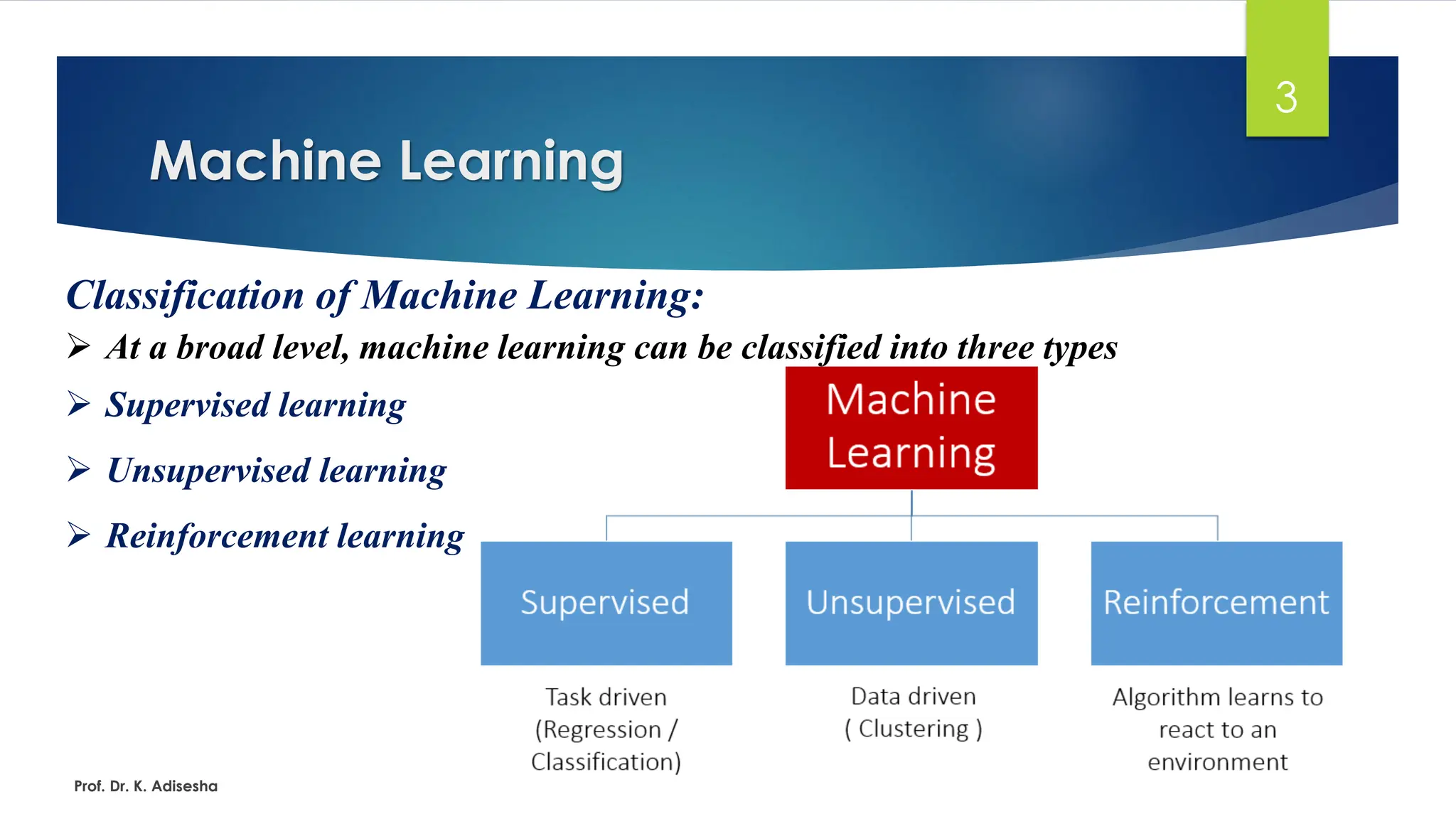
Classification ofMachine Learning:
➢ At a broad level, machine learning can be classified into three types
➢ Supervised learning
➢ Unsupervised learning
➢ Reinforcement learning
Prof. Dr. K. Adisesha
4.
Machine Learning
4
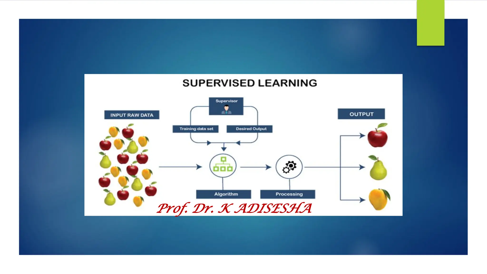
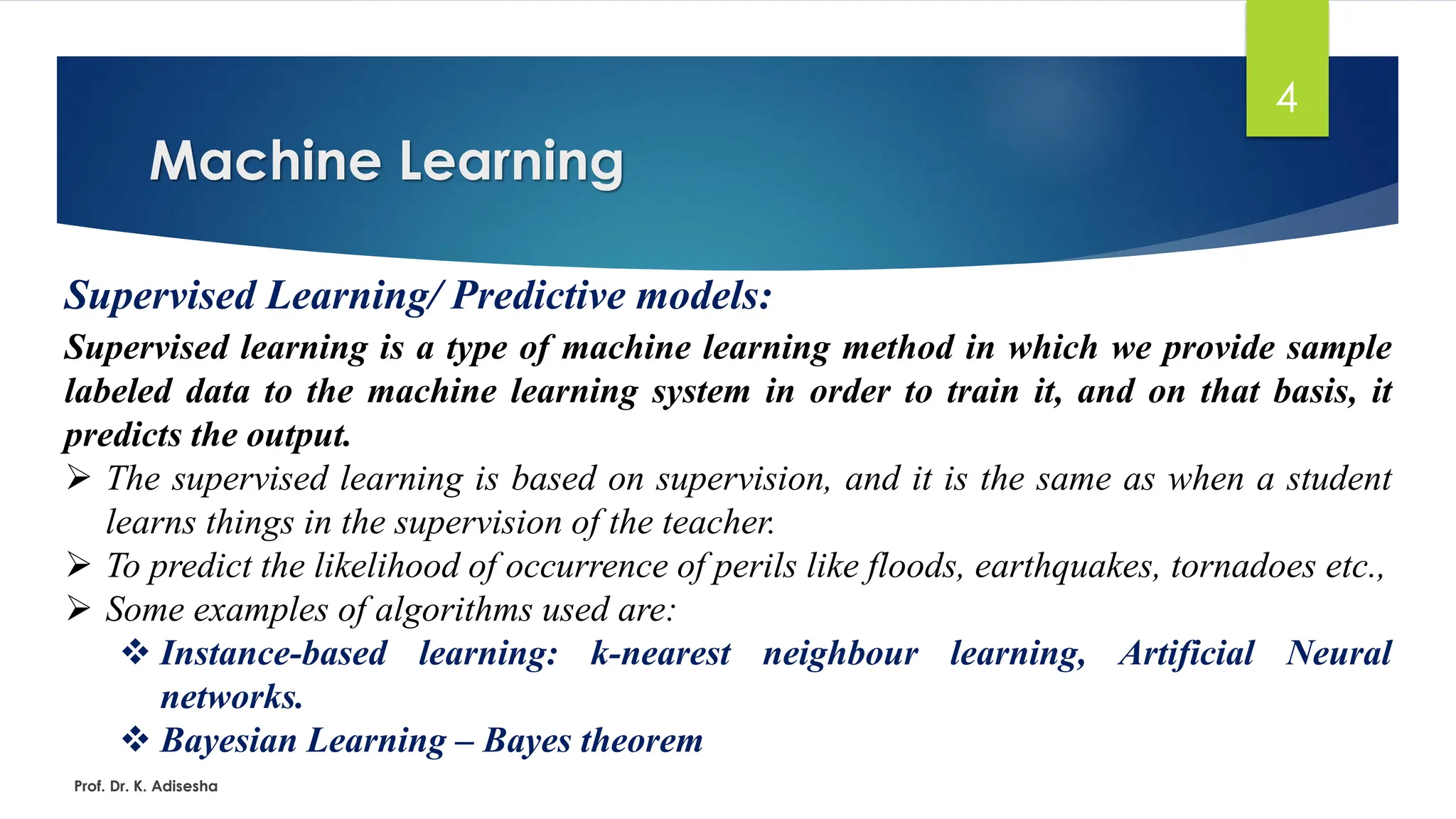
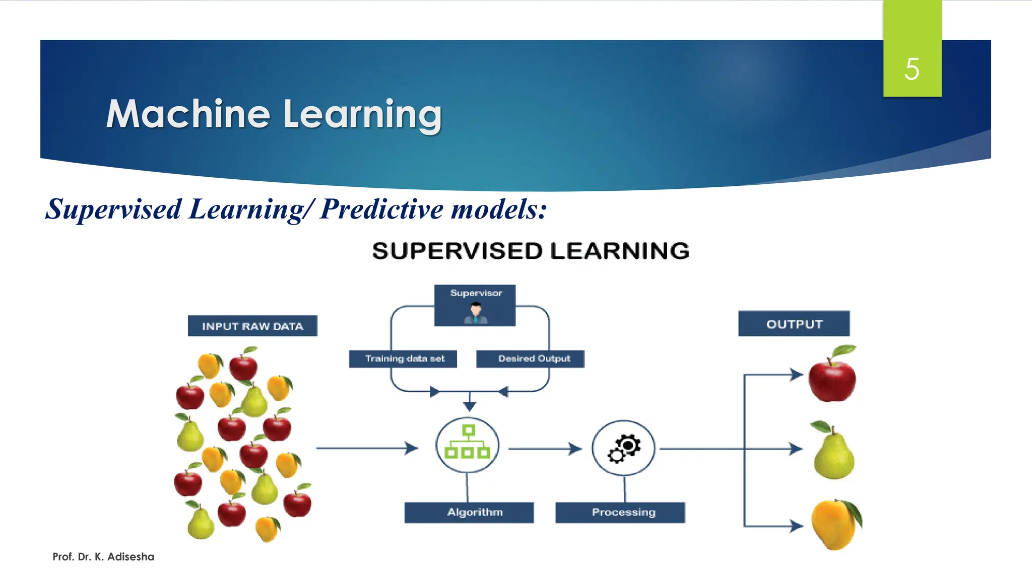
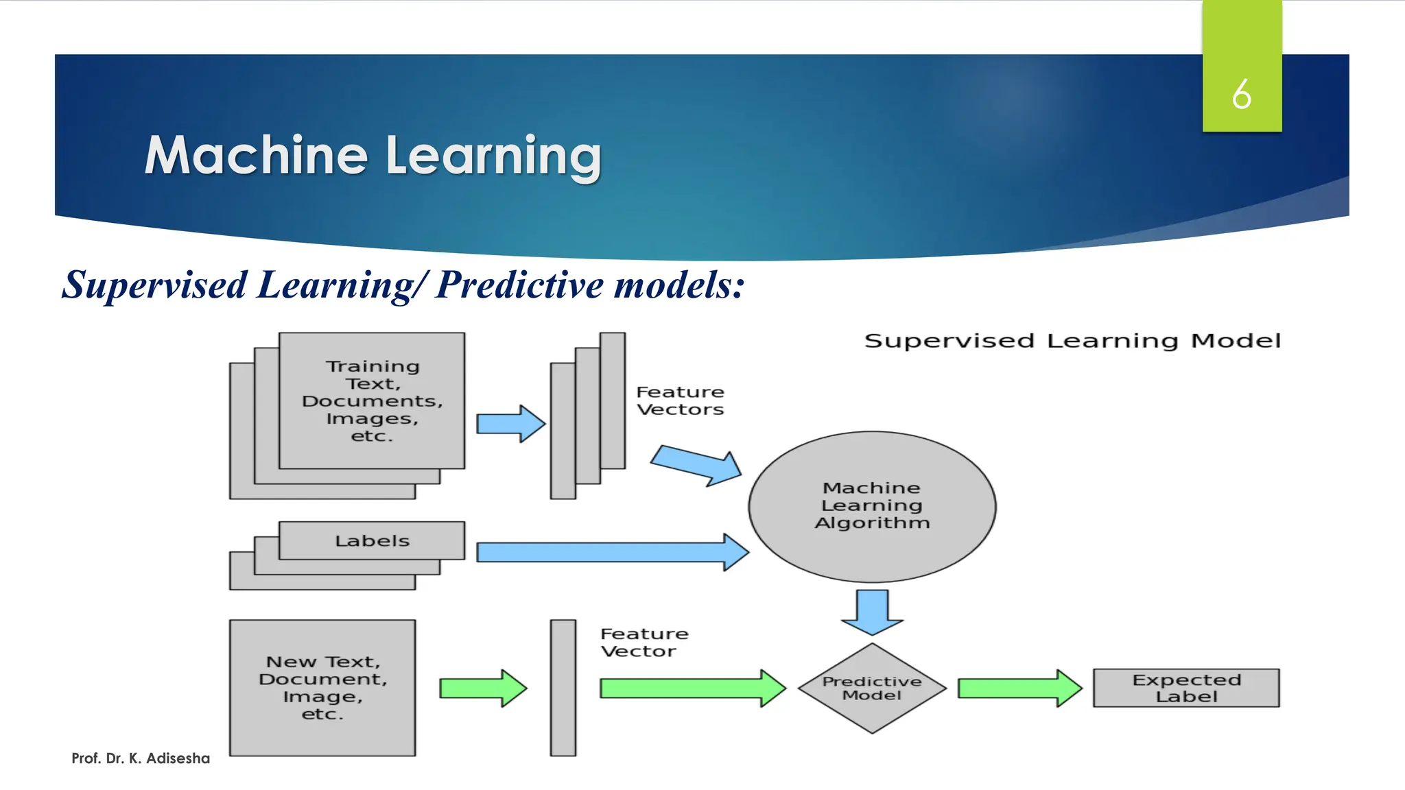
Supervised Learning/Predictive models:
Supervised learning is a type of machine learning method in which we provide sample
labeled data to the machine learning system in order to train it, and on that basis, it
predicts the output.
➢ The supervised learning is based on supervision, and it is the same as when a student
learns things in the supervision of the teacher.
➢ To predict the likelihood of occurrence of perils like floods, earthquakes, tornadoes etc.,
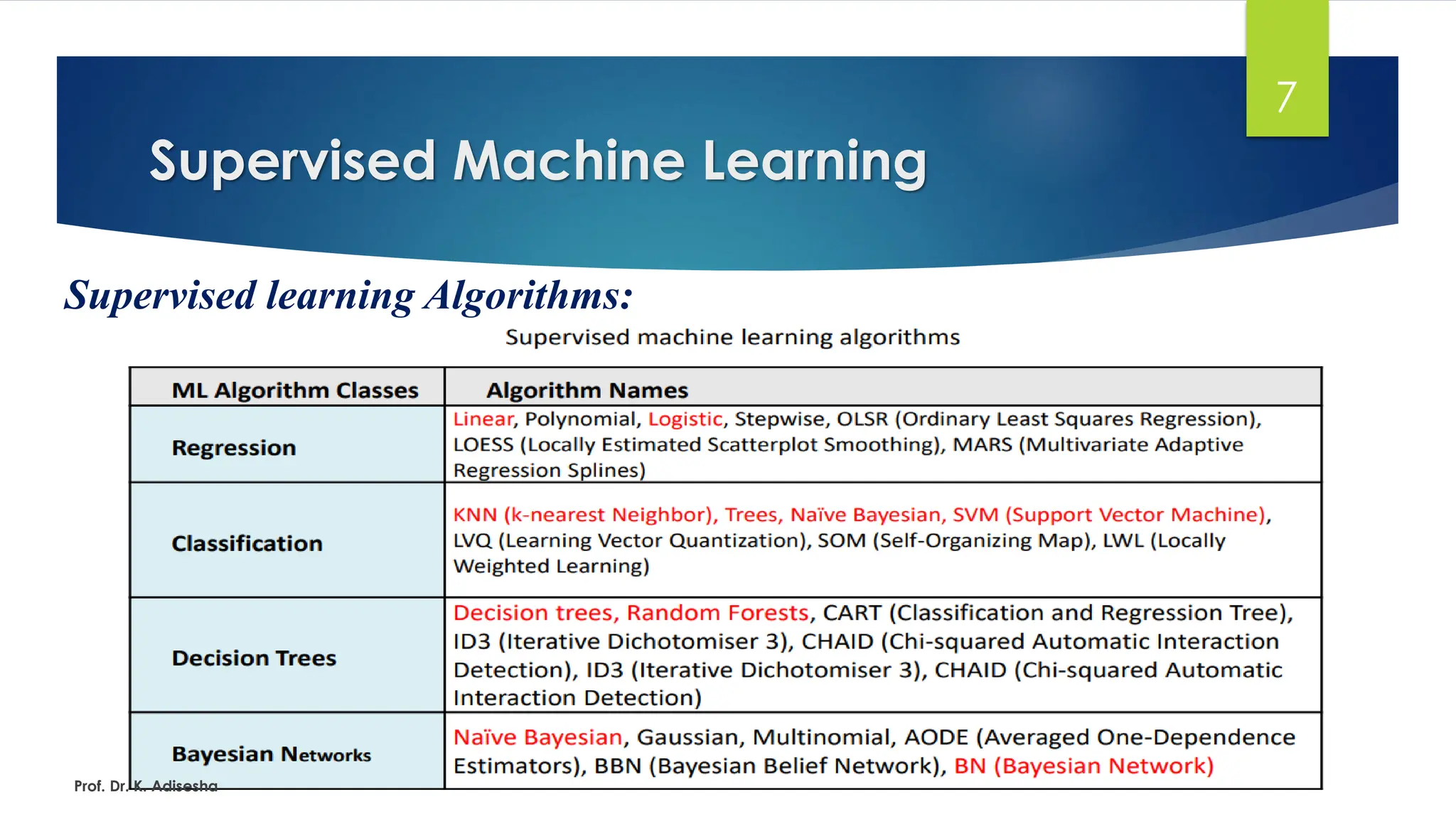
➢ Some examples of algorithms used are:
❖ Instance-based learning: k-nearest neighbour learning, Artificial Neural
networks.
❖ Bayesian Learning – Bayes theorem
Prof. Dr. K. Adisesha
Supervised Machine Learning
8
INSTANCE-BASELEARNING:
Instance-based methods are sometimes referred to as lazy learning methods because
they delay processing until a new instance must be classified.
➢ Instance-based learning methods simply store the training examples instead of
learning explicit description of the target function.
❖ Generalizing the examples is postponed until a new instance must be classified.
❖ When a new instance is encountered, its relationship to the stored examples is
examined in order to assign a target function value for the new instance.
➢ Instance-based learning includes nearest neighbor, locally weighted regression and
case-based reasoning methods.
Prof. Dr. K. Adisesha
9.
k-Nearest Neighbor Learning
9
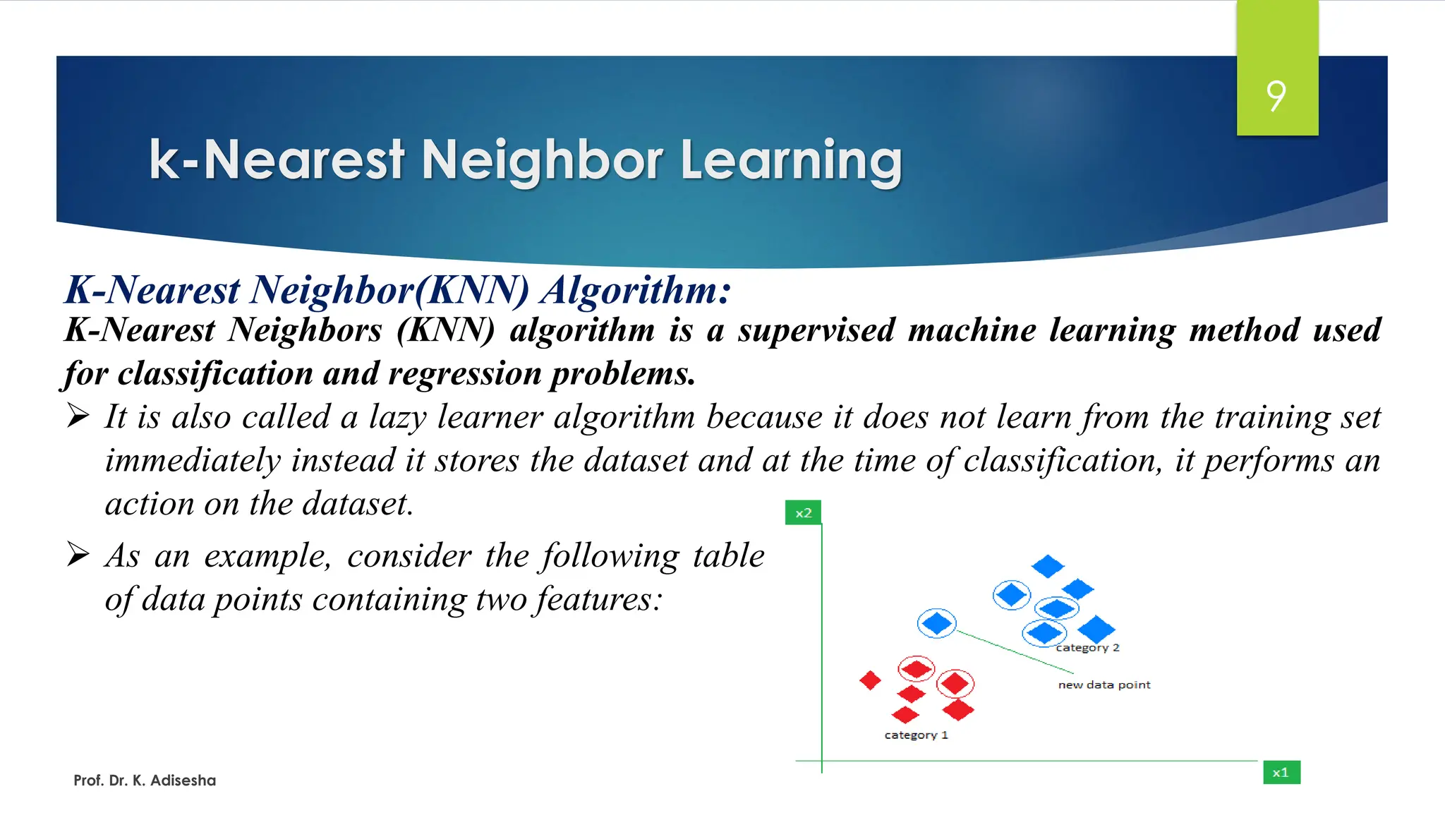
K-NearestNeighbor(KNN) Algorithm:
K-Nearest Neighbors (KNN) algorithm is a supervised machine learning method used
for classification and regression problems.
➢ It is also called a lazy learner algorithm because it does not learn from the training set
immediately instead it stores the dataset and at the time of classification, it performs an
action on the dataset.
Prof. Dr. K. Adisesha
➢ As an example, consider the following table
of data points containing two features:
10.
k-Nearest Neighbor Learning
10
K-NearestNeighbor(KNN) Algorithm:
K-Nearest Neighbors (KNN) algorithm is used for classification and regression
problems for following cases:
➢ Easy to Understand: It’s based on the simple idea of “things that are close together are
similar”
➢ Flexible: It works for:
❖ Classification: For example, is this email spam or not?
❖ Regression: For example, predicting house prices based on nearby similar houses.
➢ No Training Required: Unlike other algorithms k-NN doesn’t require a long training
process. It just stores the data and finds neighbours when needed.
➢ Works Well for Small Data: It’s effective for smaller datasets where relationships are
clear.
Prof. Dr. K. Adisesha
11.
k-Nearest Neighbor Learning
11
K-NearestNeighbor(KNN) Algorithm:
The K-NN working can be explained on the basis of the below algorithm:
➢ Step-1: Select the number K of the neighbors
➢ Step-2: Calculate the Euclidean distance of K number of neighbors
➢ Step-3: Take the K nearest neighbors as per the calculated Euclidean distance.
➢ Step-4: Among these k neighbors, count the number of the data points in each category.
➢ Step-5: Assign the new data points to that category for which the number of the
neighbor is maximum.
➢ Step-6: Our model is ready.
Prof. Dr. K. Adisesha
12.
k-Nearest Neighbor Learning
12
K-NearestNeighbor(KNN) Algorithm:
The K-NN working can be explained on the basis of the below algorithm:
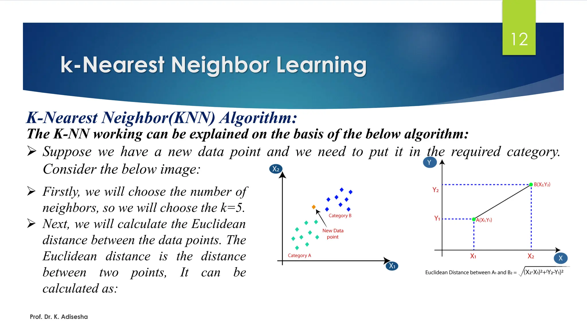
➢ Suppose we have a new data point and we need to put it in the required category.
Consider the below image:
Prof. Dr. K. Adisesha
➢ Firstly, we will choose the number of
neighbors, so we will choose the k=5.
➢ Next, we will calculate the Euclidean
distance between the data points. The
Euclidean distance is the distance
between two points, It can be
calculated as:
13.
k-Nearest Neighbor Learning
13
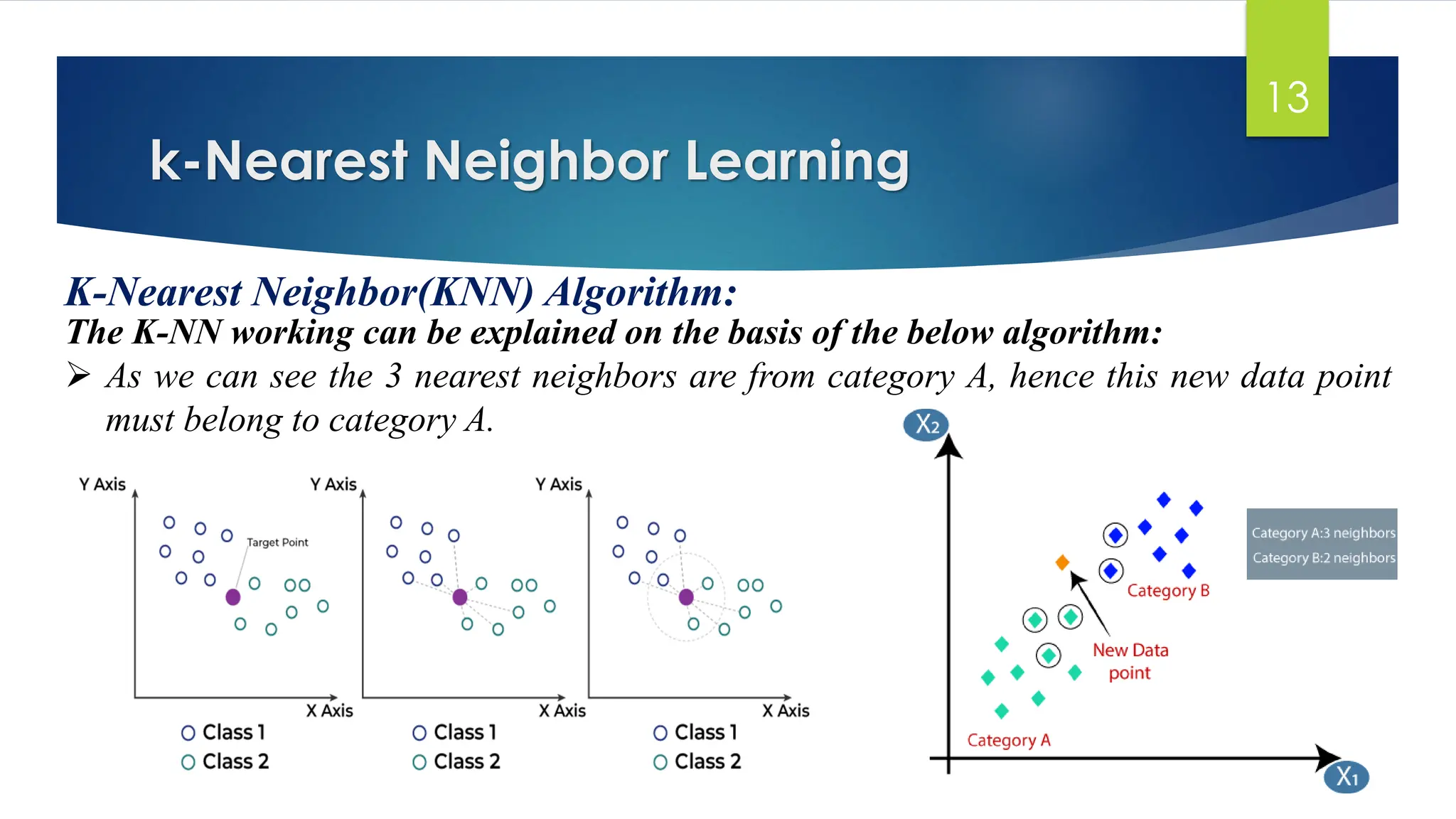
K-NearestNeighbor(KNN) Algorithm:
The K-NN working can be explained on the basis of the below algorithm:
➢ As we can see the 3 nearest neighbors are from category A, hence this new data point
must belong to category A.
Prof. Dr. K. Adisesha
14.
k-Nearest Neighbor Learning
14
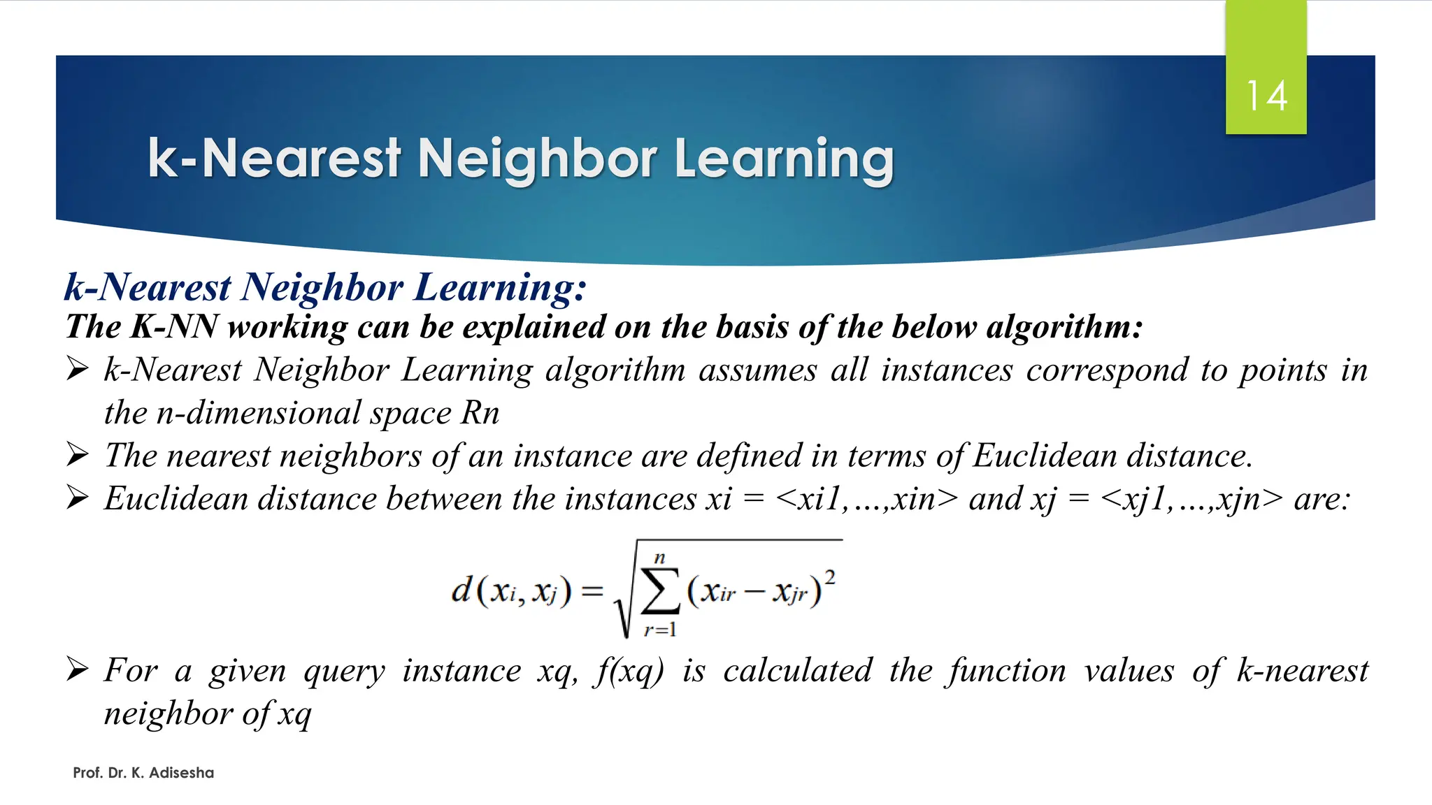
k-NearestNeighbor Learning:
The K-NN working can be explained on the basis of the below algorithm:
➢ k-Nearest Neighbor Learning algorithm assumes all instances correspond to points in
the n-dimensional space Rn
➢ The nearest neighbors of an instance are defined in terms of Euclidean distance.
➢ Euclidean distance between the instances xi = <xi1,…,xin> and xj = <xj1,…,xjn> are:
➢ For a given query instance xq, f(xq) is calculated the function values of k-nearest
neighbor of xq
Prof. Dr. K. Adisesha
15.
k-Nearest Neighbor Learning
15
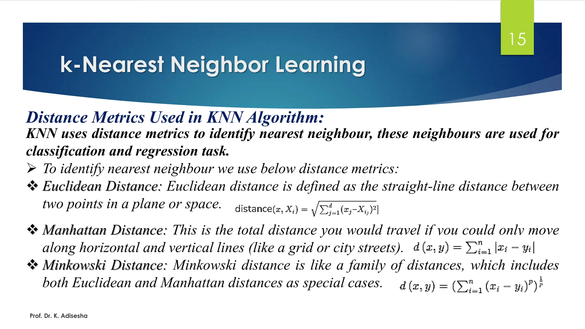
DistanceMetrics Used in KNN Algorithm:
KNN uses distance metrics to identify nearest neighbour, these neighbours are used for
classification and regression task.
➢ To identify nearest neighbour we use below distance metrics:
❖ Euclidean Distance: Euclidean distance is defined as the straight-line distance between
two points in a plane or space.
❖ Manhattan Distance: This is the total distance you would travel if you could only move
along horizontal and vertical lines (like a grid or city streets).
❖ Minkowski Distance: Minkowski distance is like a family of distances, which includes
both Euclidean and Manhattan distances as special cases.
Prof. Dr. K. Adisesha
16.
k-Nearest Neighbor Learning
16
k-NearestNeighbor Learning:
The K-NN working can be explained on the basis of the below algorithm:
Prof. Dr. K. Adisesha
➢ Advantages of KNN Algorithm:
❖ It is simple to implement.
❖ It is robust to the noisy training data
❖ It can be more effective if the training data is large.
➢ Disadvantages of KNN Algorithm:
❖ Always needs to determine the value of K which may be complex some time.
❖ The computation cost is high because of calculating the distance between the data
points for all the training samples.
17.
k-Nearest Neighbor Learning
17
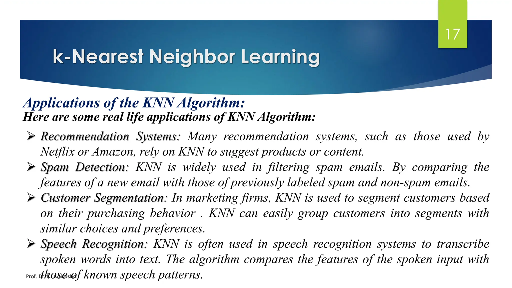
Applicationsof the KNN Algorithm:
Here are some real life applications of KNN Algorithm:
Prof. Dr. K. Adisesha
➢ Recommendation Systems: Many recommendation systems, such as those used by
Netflix or Amazon, rely on KNN to suggest products or content.
➢ Spam Detection: KNN is widely used in filtering spam emails. By comparing the
features of a new email with those of previously labeled spam and non-spam emails.
➢ Customer Segmentation: In marketing firms, KNN is used to segment customers based
on their purchasing behavior . KNN can easily group customers into segments with
similar choices and preferences.
➢ Speech Recognition: KNN is often used in speech recognition systems to transcribe
spoken words into text. The algorithm compares the features of the spoken input with
those of known speech patterns.
18.
Artificial Neural networks
18
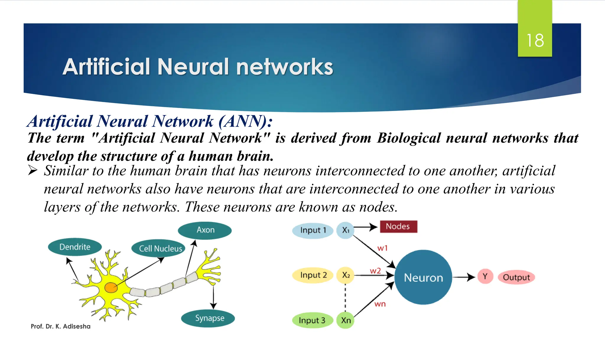
ArtificialNeural Network (ANN):
The term "Artificial Neural Network" is derived from Biological neural networks that
develop the structure of a human brain.
Prof. Dr. K. Adisesha
➢ Similar to the human brain that has neurons interconnected to one another, artificial
neural networks also have neurons that are interconnected to one another in various
layers of the networks. These neurons are known as nodes.
19.
Artificial Neural networks
19
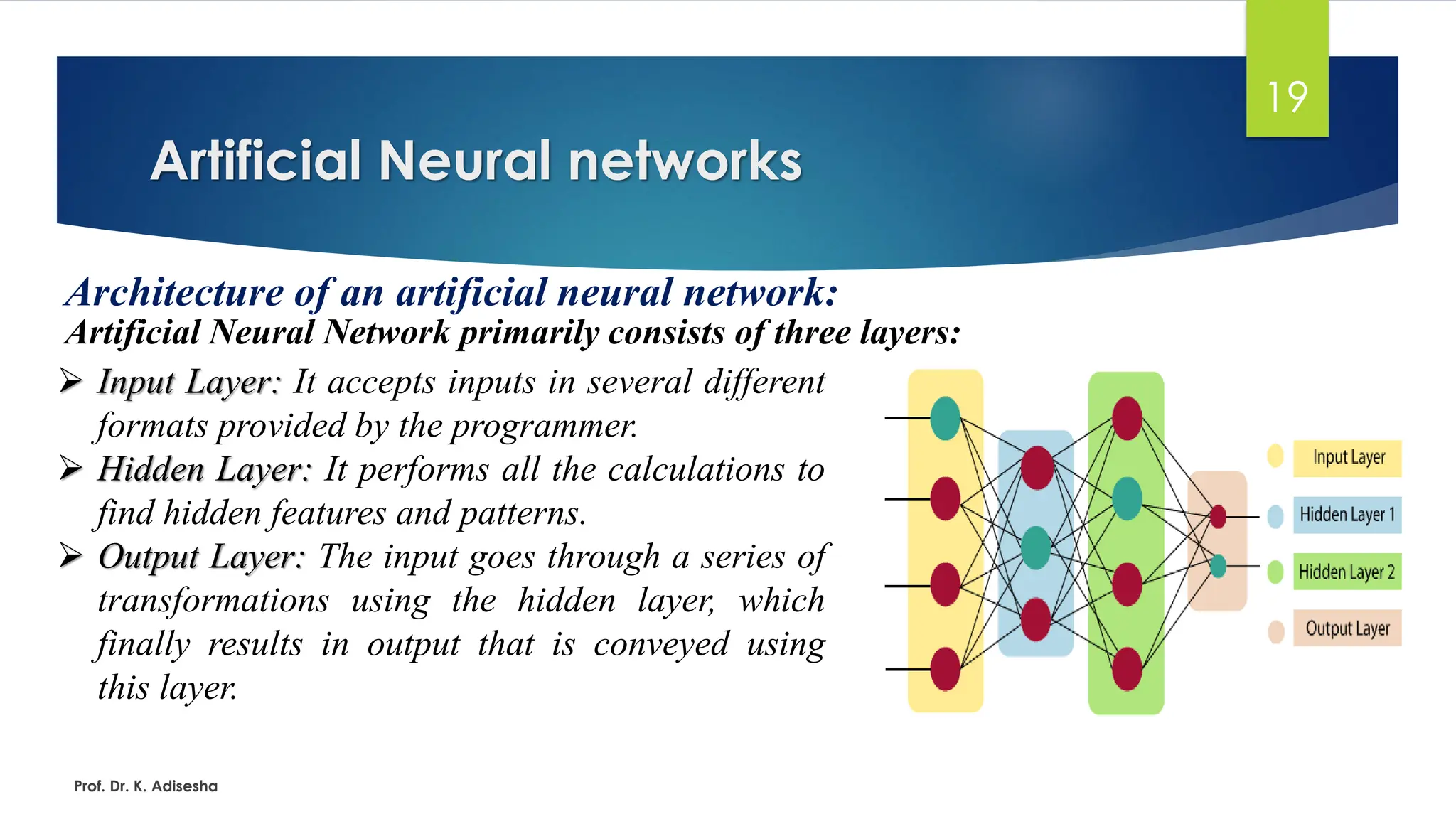
Architectureof an artificial neural network:
Artificial Neural Network primarily consists of three layers:
Prof. Dr. K. Adisesha
➢ Input Layer: It accepts inputs in several different
formats provided by the programmer.
➢ Hidden Layer: It performs all the calculations to
find hidden features and patterns.
➢ Output Layer: The input goes through a series of
transformations using the hidden layer, which
finally results in output that is conveyed using
this layer.
20.
Artificial Neural networks
20
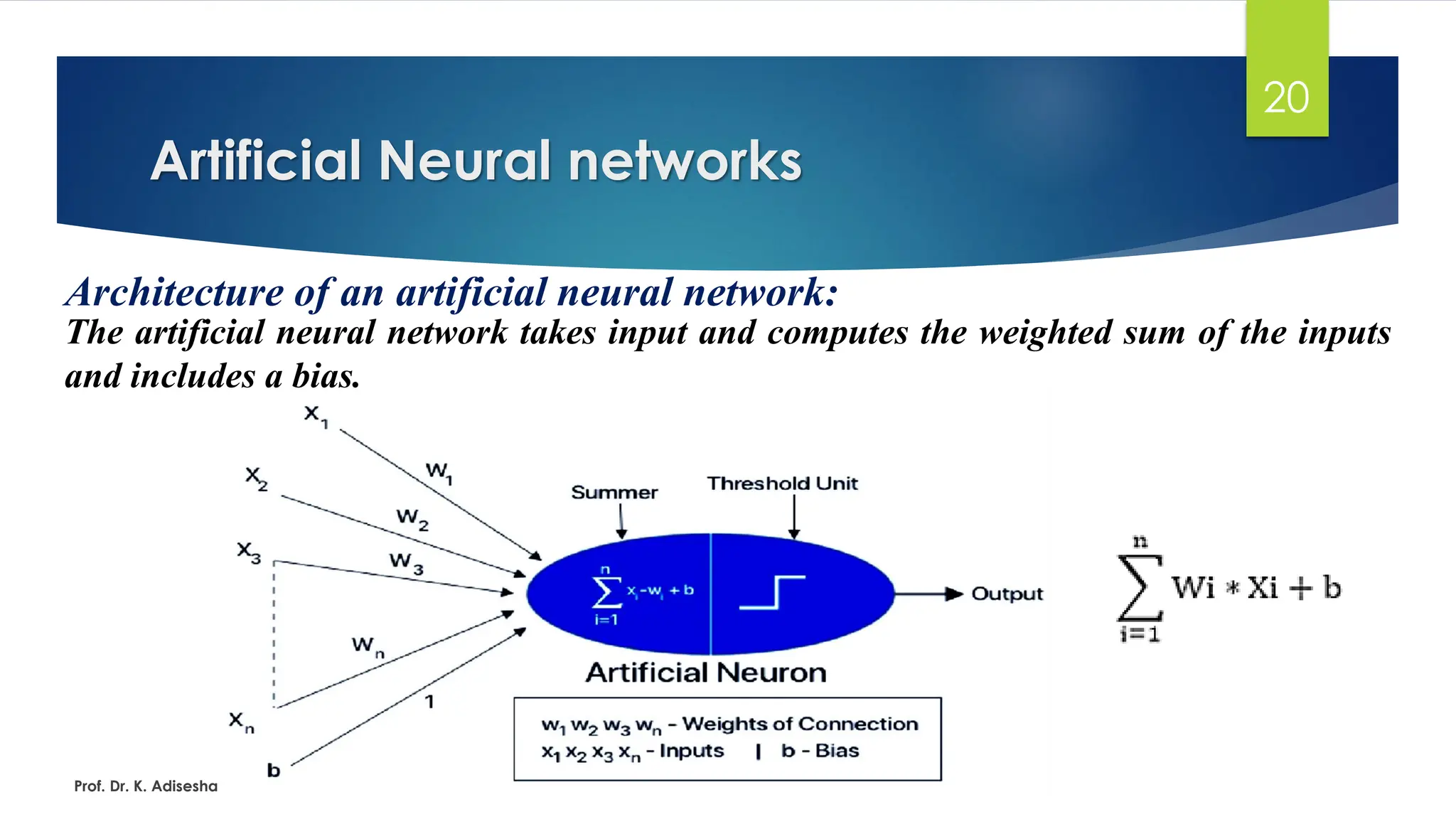
Architectureof an artificial neural network:
The artificial neural network takes input and computes the weighted sum of the inputs
and includes a bias.
Prof. Dr. K. Adisesha
21.
Artificial Neural networks
21
Commonlyused activation functions:
Some of the commonly used activation functions are binary, sigmoidal (linear), and tan
hyperbolic sigmoidal functions(nonlinear).
➢ Binary - The output has only two values, either 0 or 1. For this, the threshold value is
set up. If the net weighted input is greater than 1, the output is assumed as one;
otherwise, it is zero.
➢ Sigmoidal Hyperbolic - This function has an ‘S’ shaped curve. Here, the tan hyperbolic
function is used to approximate the output of the net input. The function is defined as –
f (x) = (1/1+ exp(-????x)) where ???? - steepness parameter.
Prof. Dr. K. Adisesha
22.
Artificial Neural networks
22
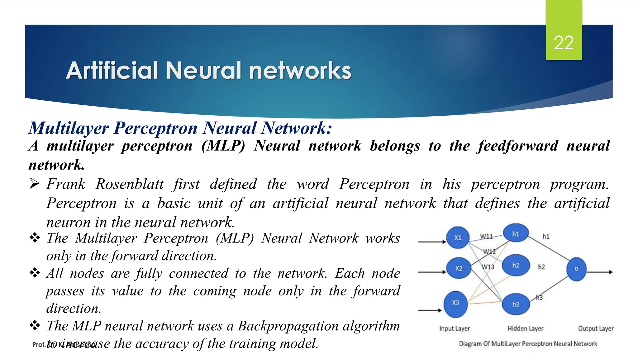
MultilayerPerceptron Neural Network:
A multilayer perceptron (MLP) Neural network belongs to the feedforward neural
network.
➢ Frank Rosenblatt first defined the word Perceptron in his perceptron program.
Perceptron is a basic unit of an artificial neural network that defines the artificial
neuron in the neural network.
Prof. Dr. K. Adisesha
❖ The Multilayer Perceptron (MLP) Neural Network works
only in the forward direction.
❖ All nodes are fully connected to the network. Each node
passes its value to the coming node only in the forward
direction.
❖ The MLP neural network uses a Backpropagation algorithm
to increase the accuracy of the training model.
23.
Artificial Neural networks
23
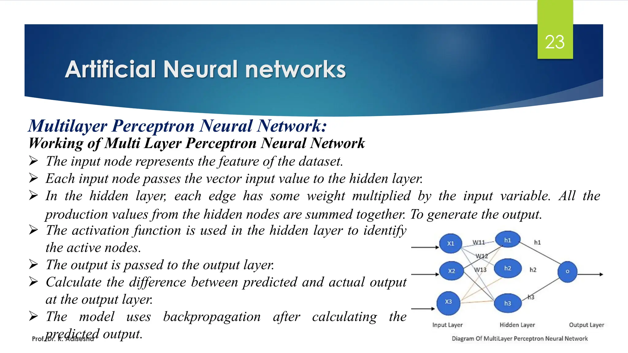
MultilayerPerceptron Neural Network:
Working of Multi Layer Perceptron Neural Network
➢ The input node represents the feature of the dataset.
➢ Each input node passes the vector input value to the hidden layer.
➢ In the hidden layer, each edge has some weight multiplied by the input variable. All the
production values from the hidden nodes are summed together. To generate the output.
Prof. Dr. K. Adisesha
➢ The activation function is used in the hidden layer to identify
the active nodes.
➢ The output is passed to the output layer.
➢ Calculate the difference between predicted and actual output
at the output layer.
➢ The model uses backpropagation after calculating the
predicted output.
24.
Artificial Neural networks
24
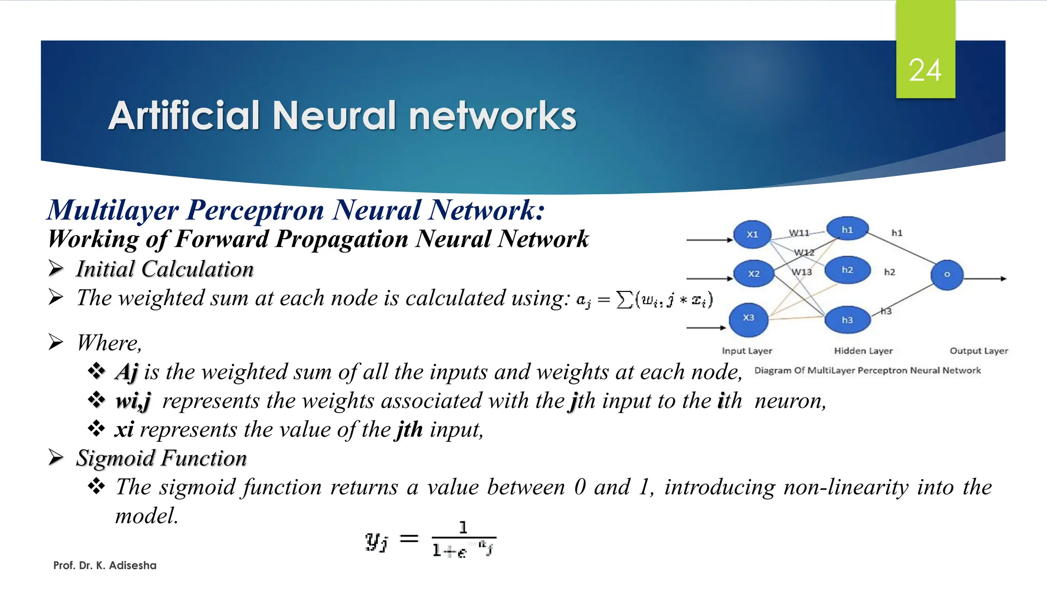
MultilayerPerceptron Neural Network:
Working of Forward Propagation Neural Network
➢ Initial Calculation
➢ The weighted sum at each node is calculated using:
Prof. Dr. K. Adisesha
➢ Where,
❖ Aj is the weighted sum of all the inputs and weights at each node,
❖ wi,j represents the weights associated with the jth input to the ith neuron,
❖ xi represents the value of the jth input,
➢ Sigmoid Function
❖ The sigmoid function returns a value between 0 and 1, introducing non-linearity into the
model.
25.
Artificial Neural networks
25
BackPropagation Algorithm:
This algorithm is used in a Multilayer perceptron neural network to increase the
accuracy of the output by reducing the error in predicted output and actual output.
➢ According to this algorithm:
❖ Calculate the error after calculating the output from the Multilayer perceptron neural network.
❖ This error is the difference between the output generated by the neural network and the actual
output. The calculated error is fed back to the network, from the output layer to the hidden
layer. Now, the output becomes the input to the network.
❖ The model reduces error by adjusting the weights in the hidden layer.
❖ Calculate the predicted output with adjusted weight and check the error. The process is
recursively used till there is minimum or no error.
❖ This algorithm helps in increasing the accuracy of the neural network.
Prof. Dr. K. Adisesha
26.
Artificial Neural networks
26
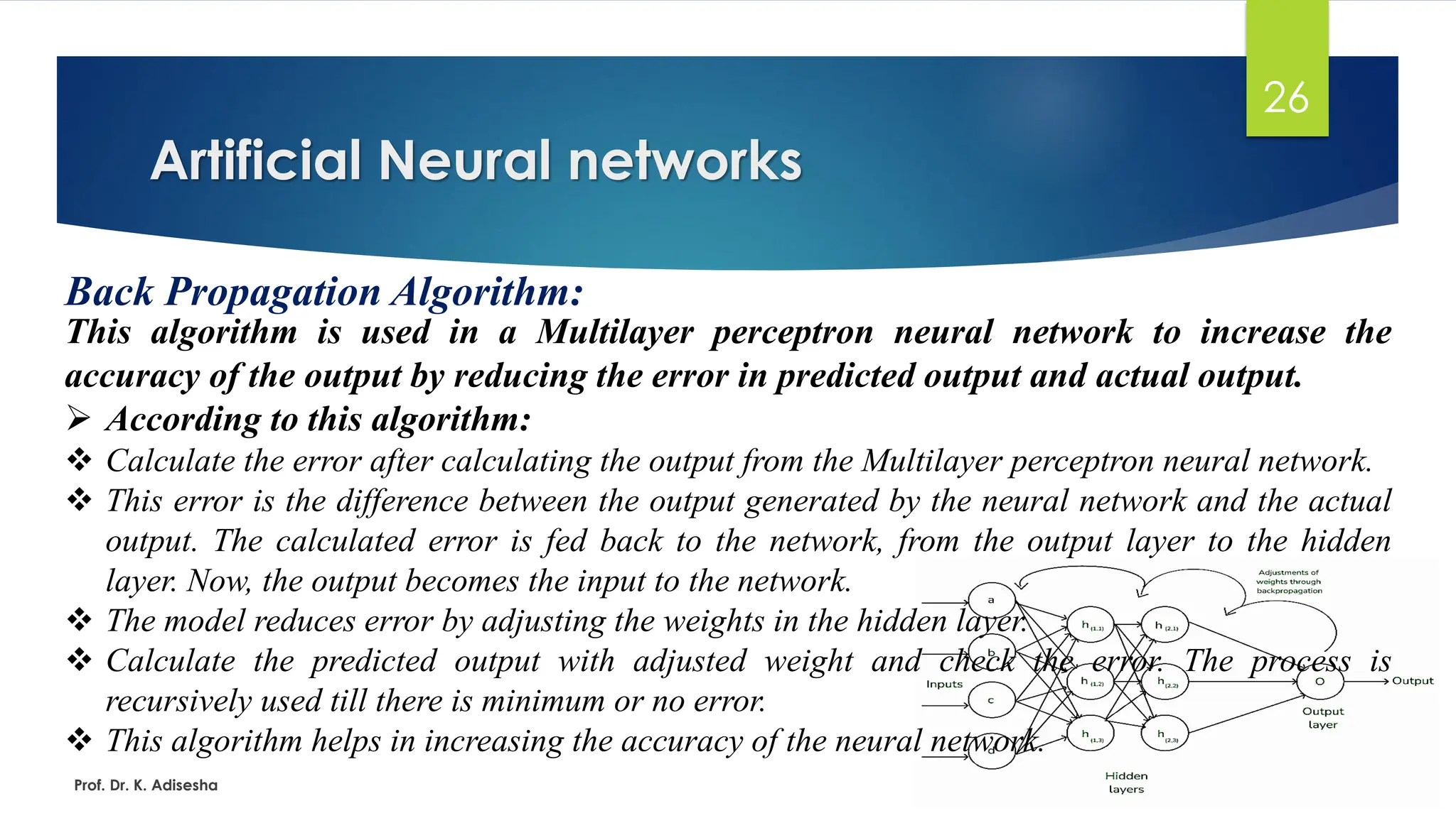
BackPropagation Algorithm:
This algorithm is used in a Multilayer perceptron neural network to increase the
accuracy of the output by reducing the error in predicted output and actual output.
➢ According to this algorithm:
❖ Calculate the error after calculating the output from the Multilayer perceptron neural network.
❖ This error is the difference between the output generated by the neural network and the actual
output. The calculated error is fed back to the network, from the output layer to the hidden
layer. Now, the output becomes the input to the network.
❖ The model reduces error by adjusting the weights in the hidden layer.
❖ Calculate the predicted output with adjusted weight and check the error. The process is
recursively used till there is minimum or no error.
❖ This algorithm helps in increasing the accuracy of the neural network.
Prof. Dr. K. Adisesha
27.
Artificial Neural networks
27
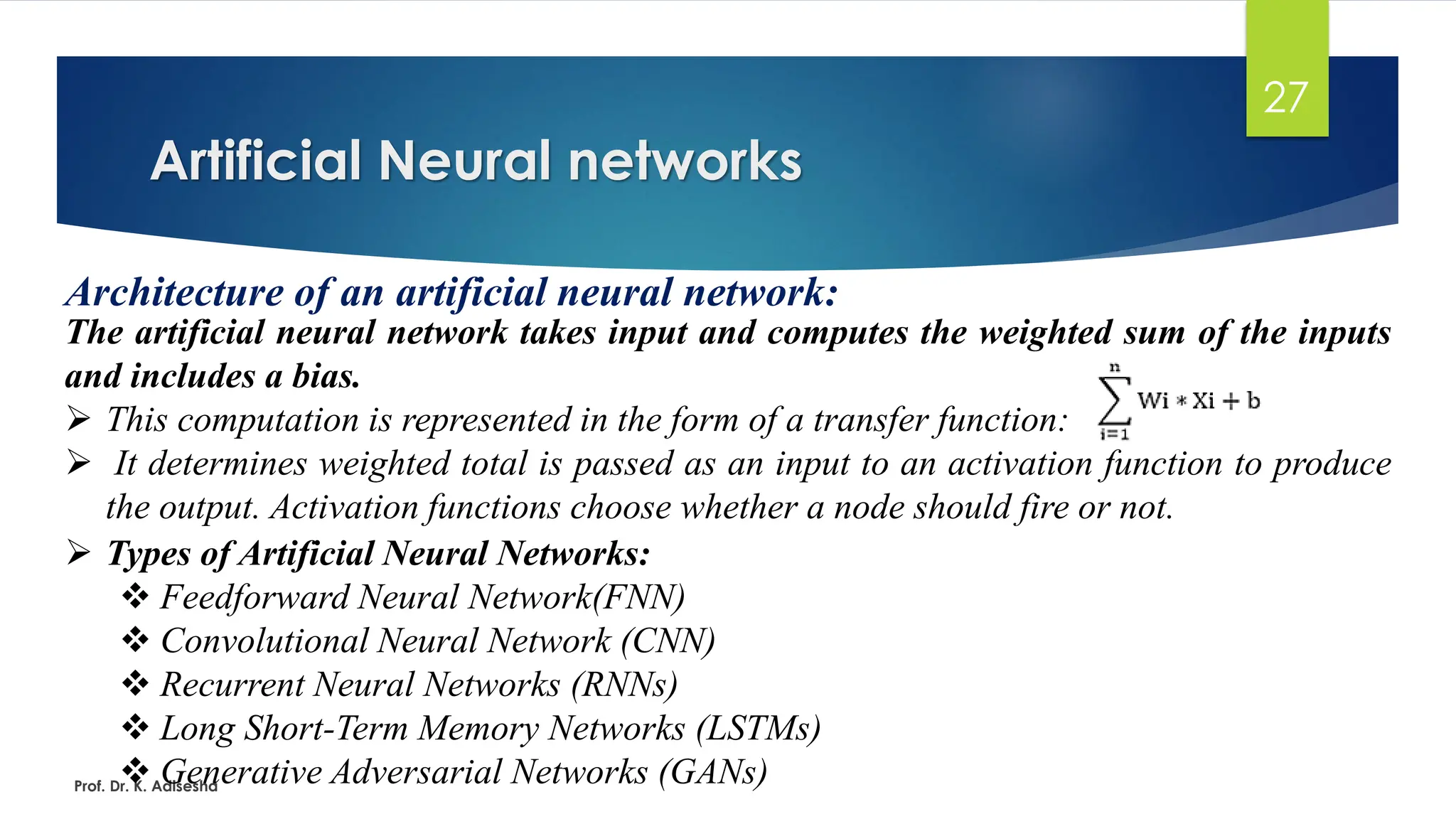
Architectureof an artificial neural network:
The artificial neural network takes input and computes the weighted sum of the inputs
and includes a bias.
➢ This computation is represented in the form of a transfer function:
➢ It determines weighted total is passed as an input to an activation function to produce
the output. Activation functions choose whether a node should fire or not.
Prof. Dr. K. Adisesha
➢ Types of Artificial Neural Networks:
❖ Feedforward Neural Network(FNN)
❖ Convolutional Neural Network (CNN)
❖ Recurrent Neural Networks (RNNs)
❖ Long Short-Term Memory Networks (LSTMs)
❖ Generative Adversarial Networks (GANs)
28.
Artificial Neural networks
28
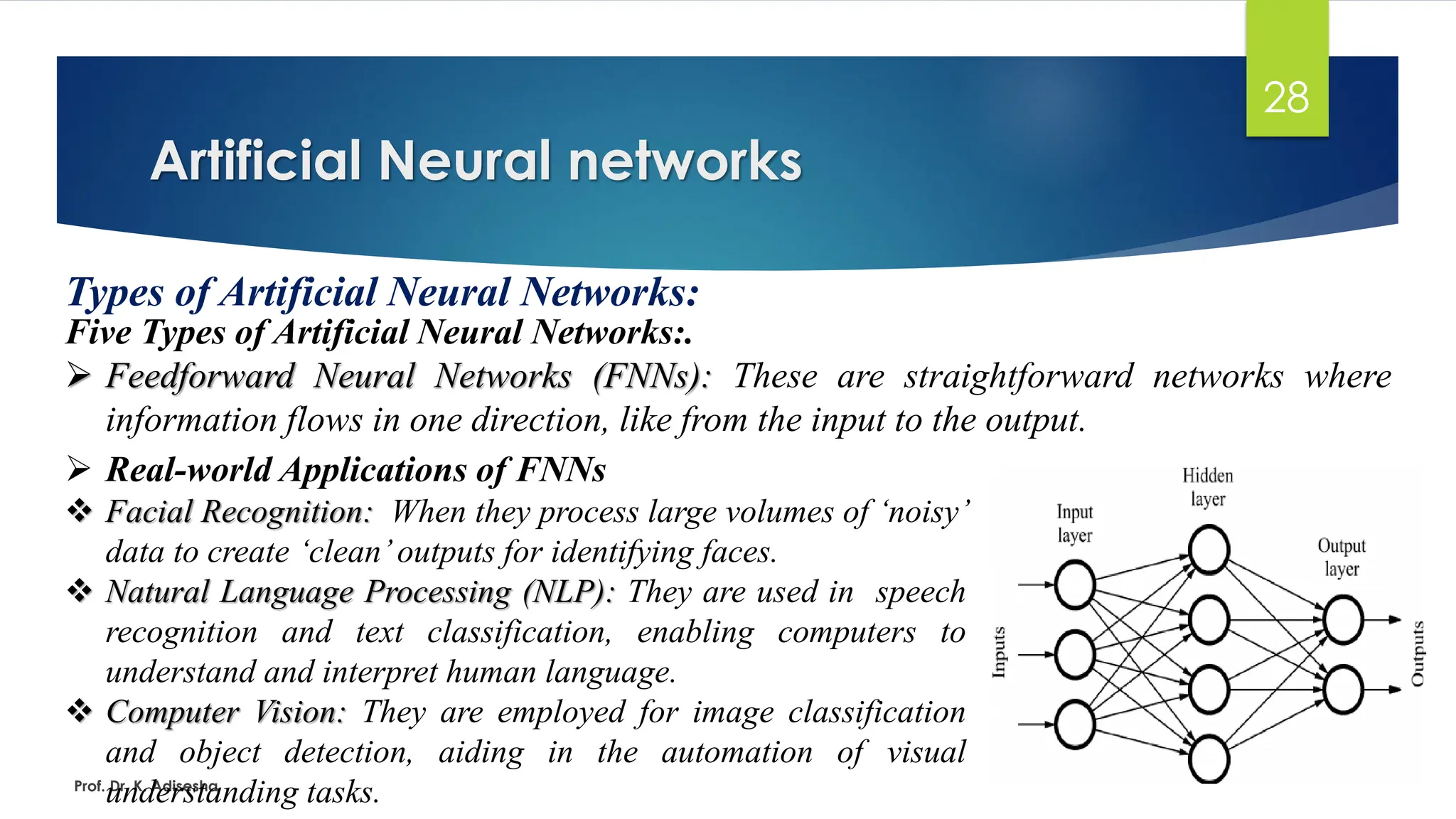
Typesof Artificial Neural Networks:
Five Types of Artificial Neural Networks:.
➢ Feedforward Neural Networks (FNNs): These are straightforward networks where
information flows in one direction, like from the input to the output.
Prof. Dr. K. Adisesha
➢ Real-world Applications of FNNs
❖ Facial Recognition: When they process large volumes of ‘noisy’
data to create ‘clean’outputs for identifying faces.
❖ Natural Language Processing (NLP): They are used in speech
recognition and text classification, enabling computers to
understand and interpret human language.
❖ Computer Vision: They are employed for image classification
and object detection, aiding in the automation of visual
understanding tasks.
29.
Artificial Neural networks
29
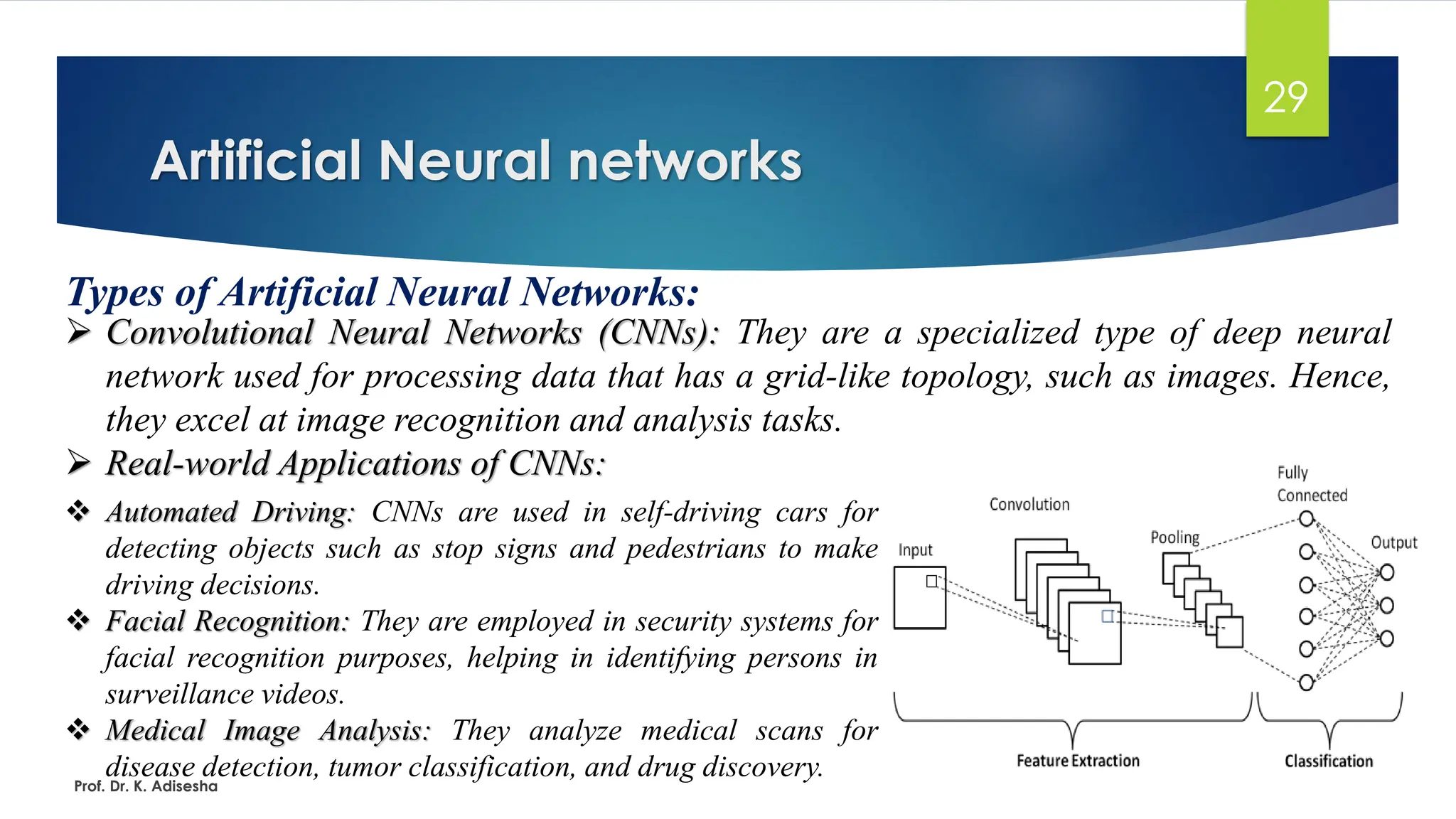
Typesof Artificial Neural Networks:
➢ Convolutional Neural Networks (CNNs): They are a specialized type of deep neural
network used for processing data that has a grid-like topology, such as images. Hence,
they excel at image recognition and analysis tasks.
➢ Real-world Applications of CNNs:
Prof. Dr. K. Adisesha
❖ Automated Driving: CNNs are used in self-driving cars for
detecting objects such as stop signs and pedestrians to make
driving decisions.
❖ Facial Recognition: They are employed in security systems for
facial recognition purposes, helping in identifying persons in
surveillance videos.
❖ Medical Image Analysis: They analyze medical scans for
disease detection, tumor classification, and drug discovery.
30.
Artificial Neural networks
30
Typesof Artificial Neural Networks:
Five Types of Artificial Neural Networks:.
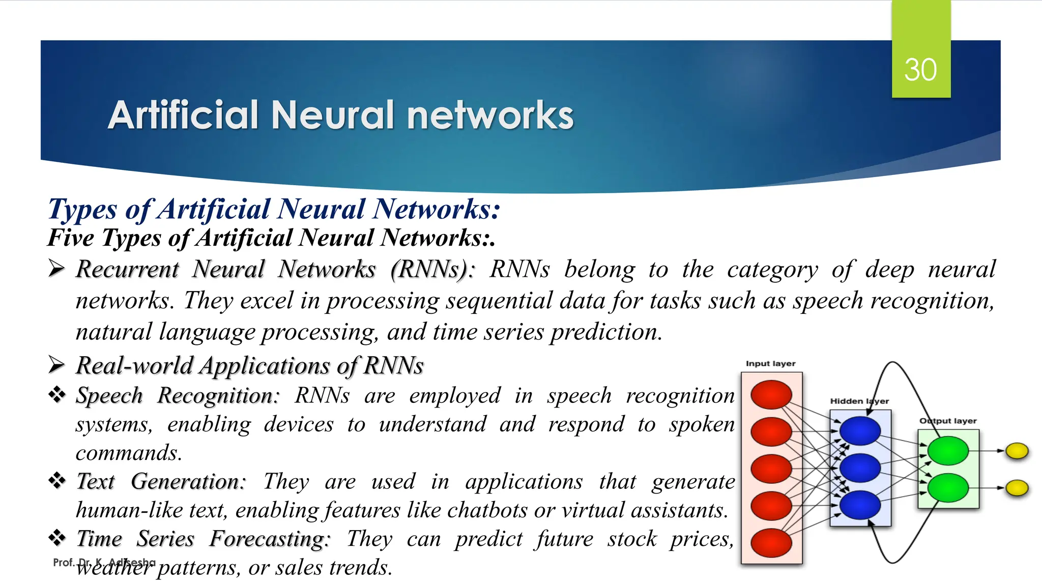
➢ Recurrent Neural Networks (RNNs): RNNs belong to the category of deep neural
networks. They excel in processing sequential data for tasks such as speech recognition,
natural language processing, and time series prediction.
Prof. Dr. K. Adisesha
➢ Real-world Applications of RNNs
❖ Speech Recognition: RNNs are employed in speech recognition
systems, enabling devices to understand and respond to spoken
commands.
❖ Text Generation: They are used in applications that generate
human-like text, enabling features like chatbots or virtual assistants.
❖ Time Series Forecasting: They can predict future stock prices,
weather patterns, or sales trends.
31.
Artificial Neural networks
31
Typesof Artificial Neural Networks:
Five Types of Artificial Neural Networks:.
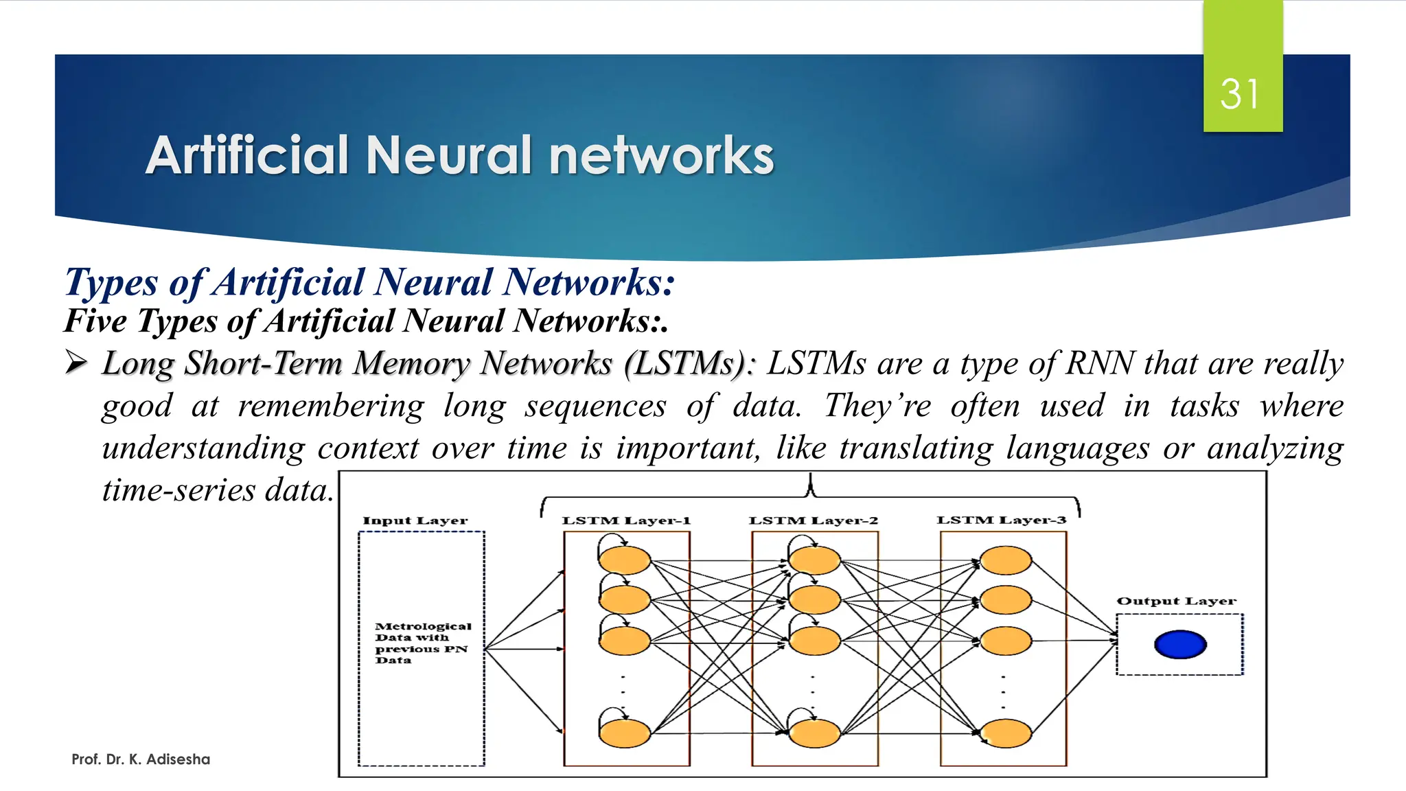
➢ Long Short-Term Memory Networks (LSTMs): LSTMs are a type of RNN that are really
good at remembering long sequences of data. They’re often used in tasks where
understanding context over time is important, like translating languages or analyzing
time-series data.
Prof. Dr. K. Adisesha
32.
Artificial Neural networks
32
Typesof Artificial Neural Networks:
Five Types of Artificial Neural Networks:.
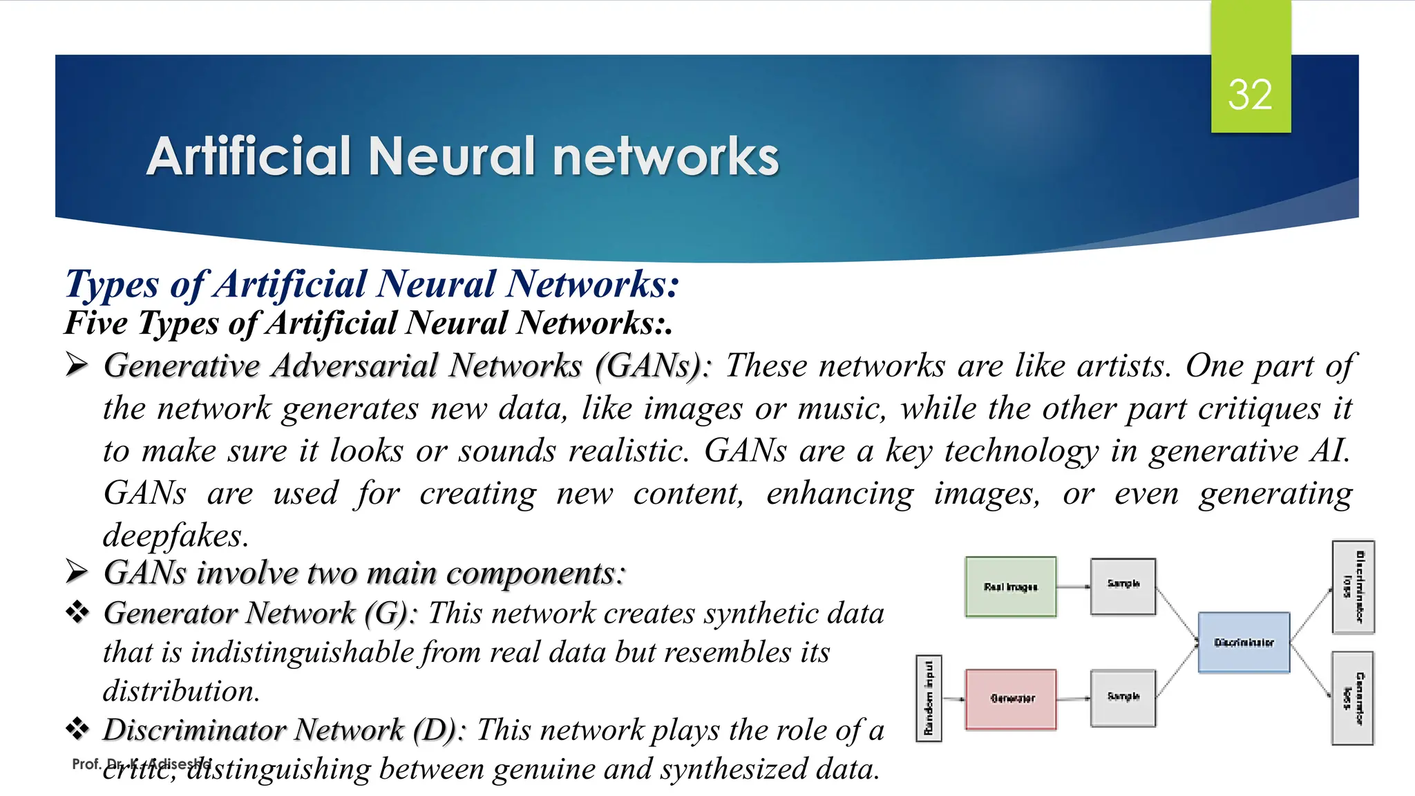
➢ Generative Adversarial Networks (GANs): These networks are like artists. One part of
the network generates new data, like images or music, while the other part critiques it
to make sure it looks or sounds realistic. GANs are a key technology in generative AI.
GANs are used for creating new content, enhancing images, or even generating
deepfakes.
Prof. Dr. K. Adisesha
➢ GANs involve two main components:
❖ Generator Network (G): This network creates synthetic data
that is indistinguishable from real data but resembles its
distribution.
❖ Discriminator Network (D): This network plays the role of a
critic, distinguishing between genuine and synthesized data.
33.
Artificial Neural networks
33
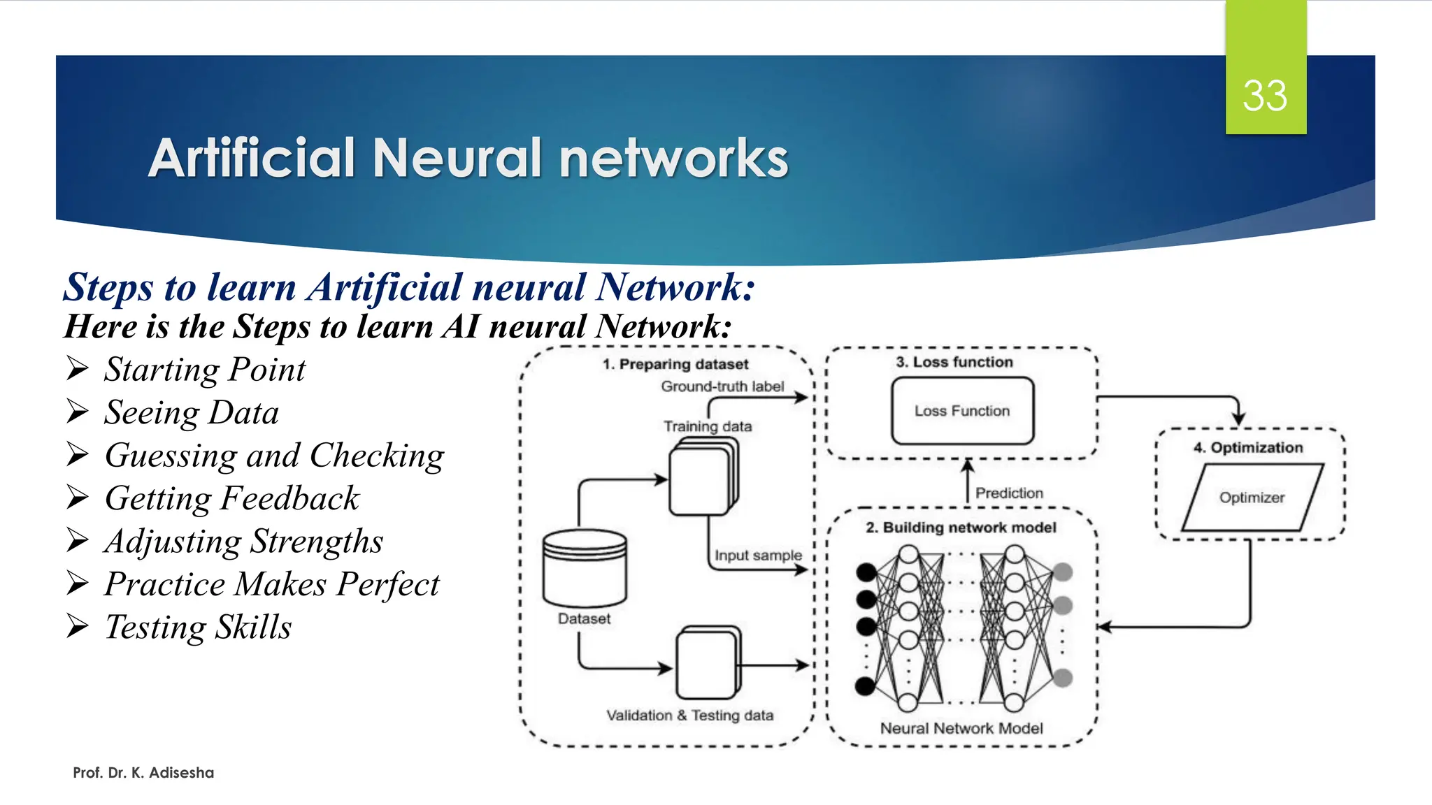
Stepsto learn Artificial neural Network:
Here is the Steps to learn AI neural Network:
➢ Starting Point
➢ Seeing Data
➢ Guessing and Checking
➢ Getting Feedback
➢ Adjusting Strengths
➢ Practice Makes Perfect
➢ Testing Skills
Prof. Dr. K. Adisesha
34.
Artificial Neural networks
34
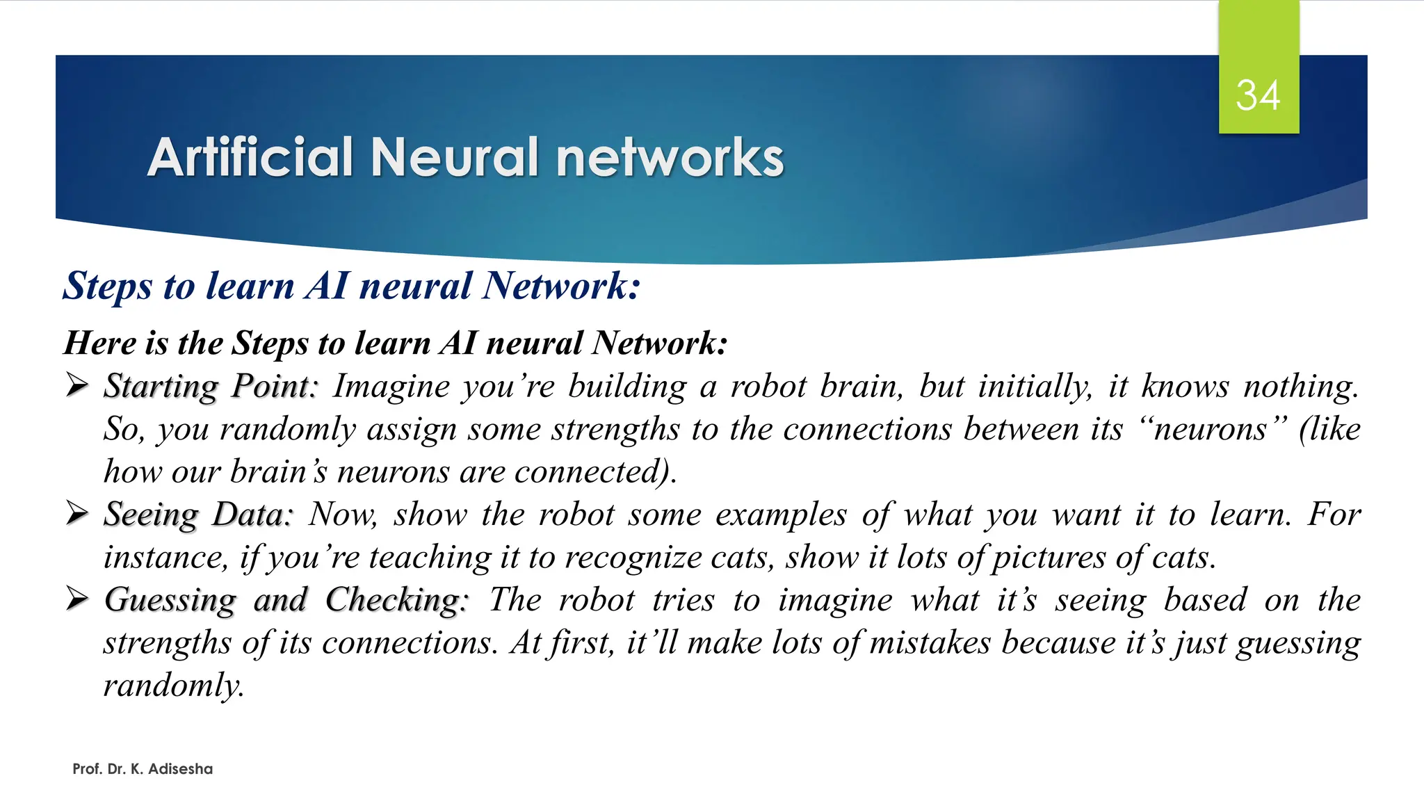
Stepsto learn AI neural Network:
Here is the Steps to learn AI neural Network:
➢ Starting Point: Imagine you’re building a robot brain, but initially, it knows nothing.
So, you randomly assign some strengths to the connections between its “neurons” (like
how our brain’s neurons are connected).
➢ Seeing Data: Now, show the robot some examples of what you want it to learn. For
instance, if you’re teaching it to recognize cats, show it lots of pictures of cats.
➢ Guessing and Checking: The robot tries to imagine what it’s seeing based on the
strengths of its connections. At first, it’ll make lots of mistakes because it’s just guessing
randomly.
Prof. Dr. K. Adisesha
35.
Artificial Neural networks
35
Stepsto learn Artificial Neural Networks:
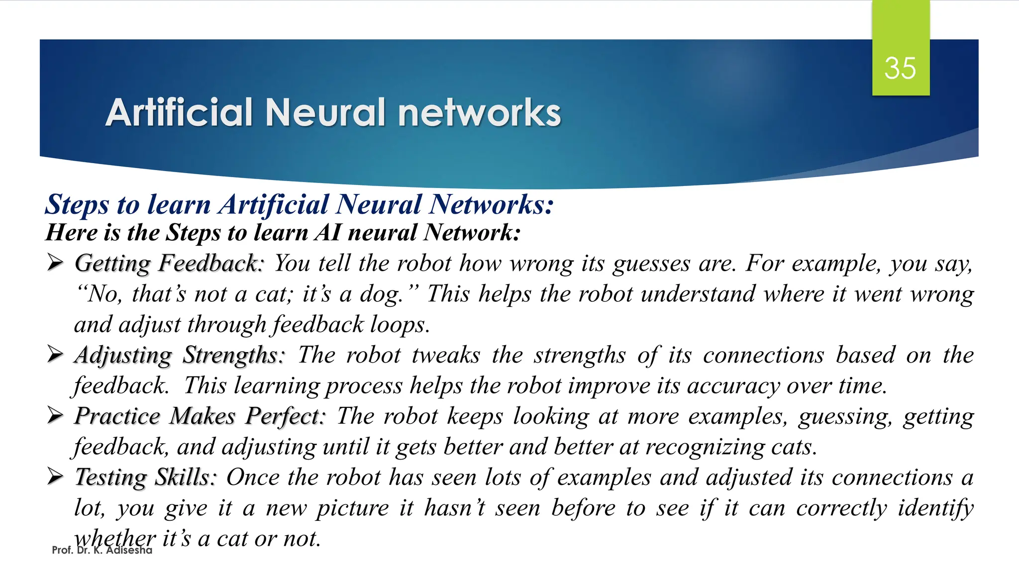
Here is the Steps to learn AI neural Network:
➢ Getting Feedback: You tell the robot how wrong its guesses are. For example, you say,
“No, that’s not a cat; it’s a dog.” This helps the robot understand where it went wrong
and adjust through feedback loops.
➢ Adjusting Strengths: The robot tweaks the strengths of its connections based on the
feedback. This learning process helps the robot improve its accuracy over time.
➢ Practice Makes Perfect: The robot keeps looking at more examples, guessing, getting
feedback, and adjusting until it gets better and better at recognizing cats.
➢ Testing Skills: Once the robot has seen lots of examples and adjusted its connections a
lot, you give it a new picture it hasn’t seen before to see if it can correctly identify
whether it’s a cat or not.
Prof. Dr. K. Adisesha
36.
Artificial Neural networks
36
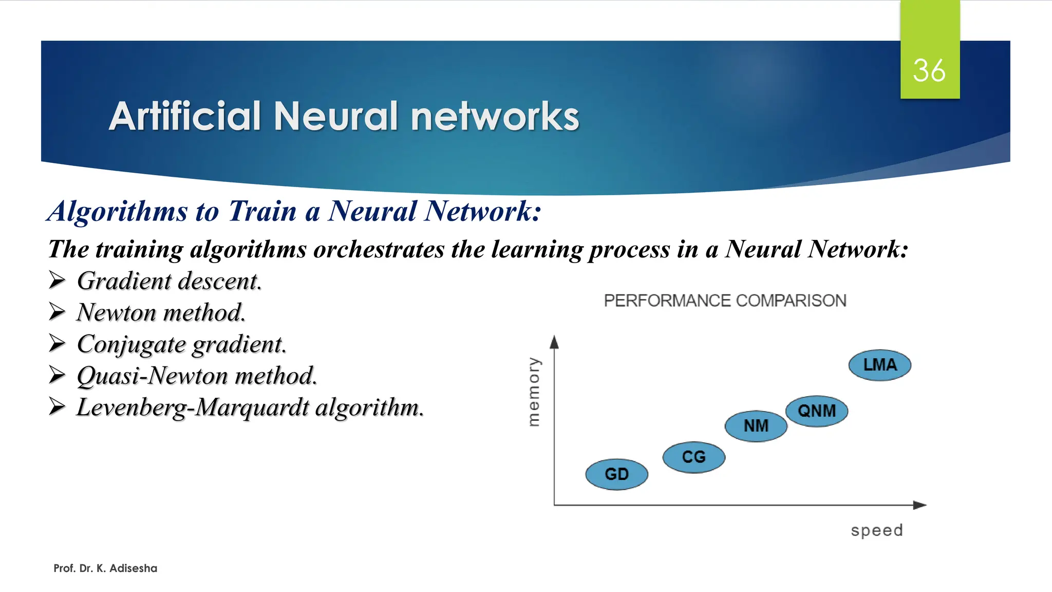
Algorithmsto Train a Neural Network:
The training algorithms orchestrates the learning process in a Neural Network:
➢ Gradient descent.
➢ Newton method.
➢ Conjugate gradient.
➢ Quasi-Newton method.
➢ Levenberg-Marquardt algorithm.
Prof. Dr. K. Adisesha
37.
Artificial Neural networks
37
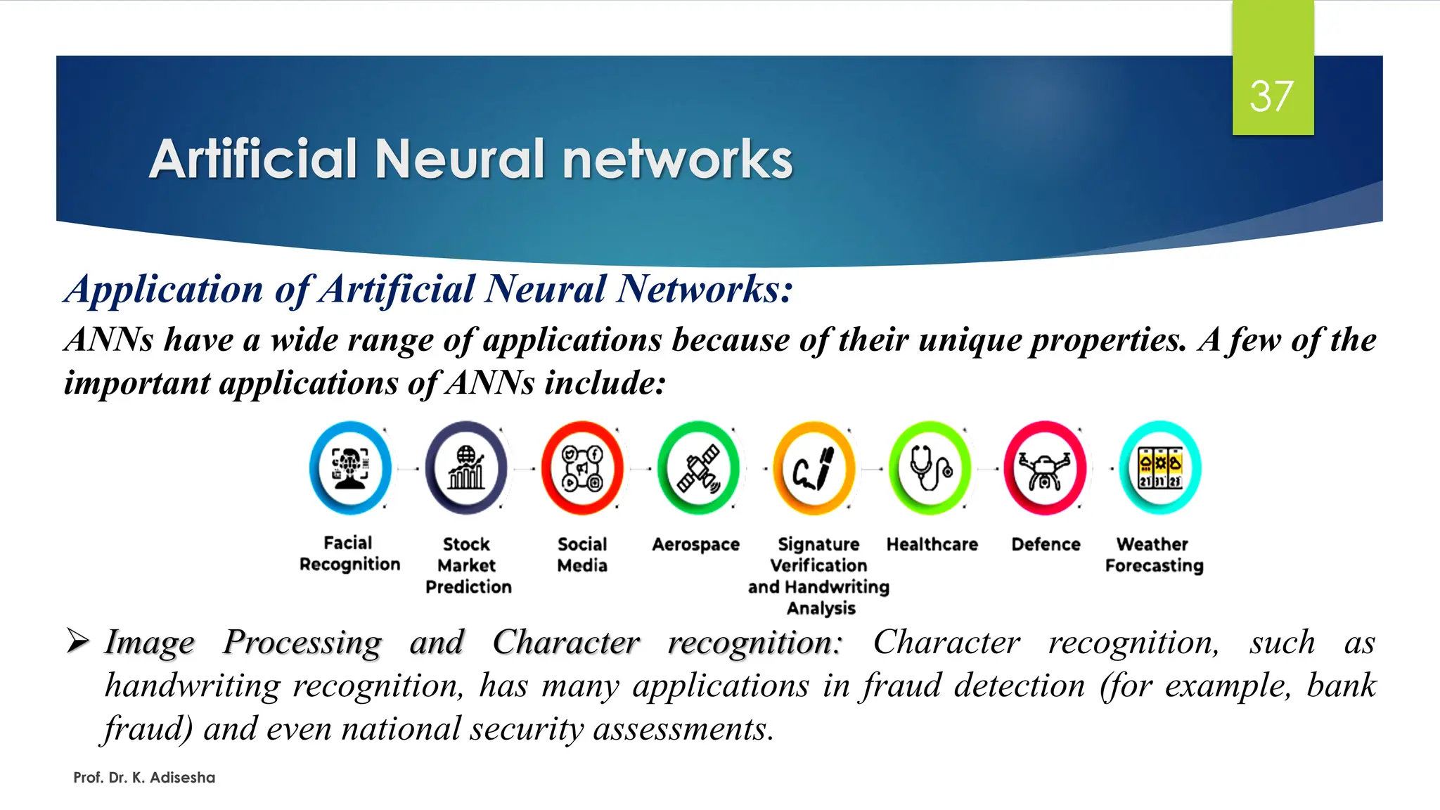
Applicationof Artificial Neural Networks:
ANNs have a wide range of applications because of their unique properties. A few of the
important applications of ANNs include:
➢ Image Processing and Character recognition: Character recognition, such as
handwriting recognition, has many applications in fraud detection (for example, bank
fraud) and even national security assessments.
Prof. Dr. K. Adisesha
38.
Artificial Neural networks
38
Applicationof Artificial Neural Networks:
ANNs have a wide range of applications because of their unique properties. A few of the
important applications of ANNs include:
➢ Facial Recognition: Facial Recognition Systems are serving as robust systems of
surveillance.
➢ Stock Market Prediction: Investments are subject to market risks. It is nearly impossible
to predict the upcoming changes in the highly volatile stock market.
➢ Social Media: Artificial Neural Networks are used to study the behaviours of social
media users.
➢ Aerospace: Aerospace Engineering is an expansive term that covers fault diagnosis,
high performance auto piloting, securing the aircraft control systems, and modeling key
Prof. Dr. K. Adisesha
39.
Artificial Neural networks
39
Theadvantages & disadvantages of Artificial Neural Networks:
The advantages are listed below:
➢ A neural network can perform tasks that a linear program can not.
➢ When an element of the neural network fails, its parallel nature can continue without
any problem.
➢ A neural network learns, and reprogramming is not necessary.
➢ It can be implemented in any application.
➢ It can be performed without any problem.
The disadvantages are described below:
➢ The neural network needs training to operate.
➢ Requires high processing time for large neural networks.
Prof. Dr. K. Adisesha
40.
Support Vector MachineAlgorithm
40
Support Vector Machine (SMV)Algorithm:
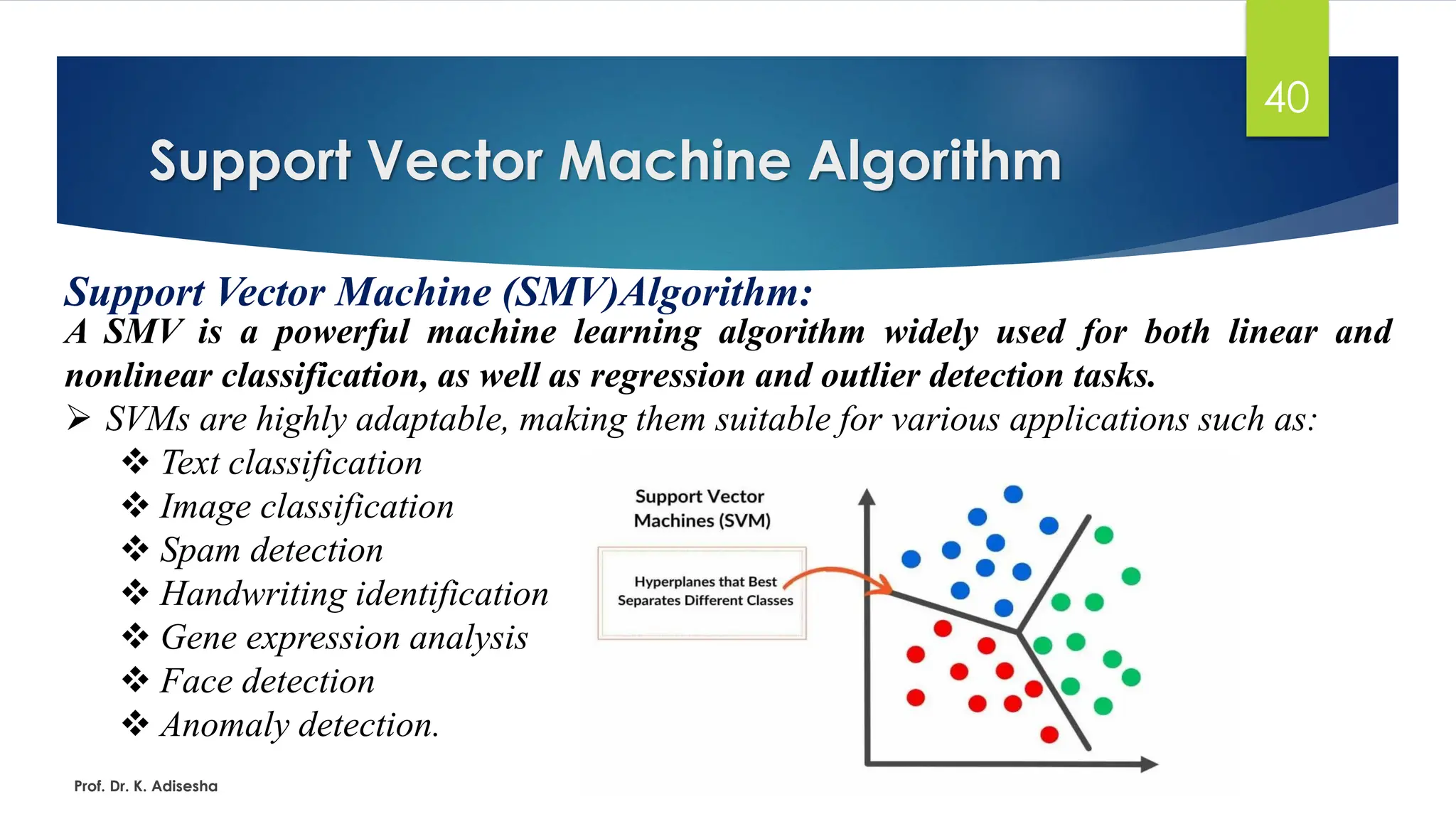
A SMV is a powerful machine learning algorithm widely used for both linear and
nonlinear classification, as well as regression and outlier detection tasks.
➢ SVMs are highly adaptable, making them suitable for various applications such as:
❖ Text classification
❖ Image classification
❖ Spam detection
❖ Handwriting identification
❖ Gene expression analysis
❖ Face detection
❖ Anomaly detection.
Prof. Dr. K. Adisesha
41.
Support Vector MachineAlgorithm
41
Support Vector Machine (SMV)Algorithm:
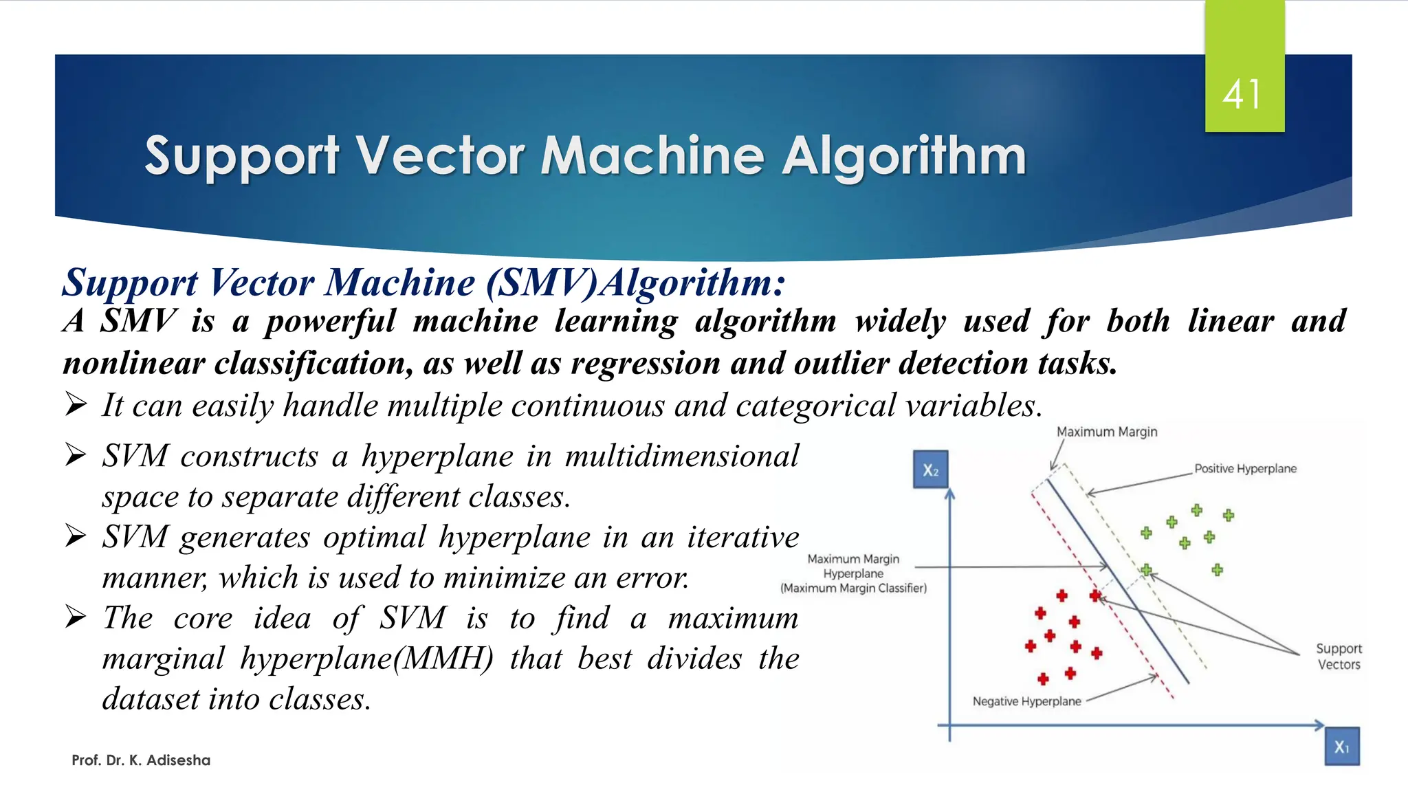
A SMV is a powerful machine learning algorithm widely used for both linear and
nonlinear classification, as well as regression and outlier detection tasks.
➢ It can easily handle multiple continuous and categorical variables.
Prof. Dr. K. Adisesha
➢ SVM constructs a hyperplane in multidimensional
space to separate different classes.
➢ SVM generates optimal hyperplane in an iterative
manner, which is used to minimize an error.
➢ The core idea of SVM is to find a maximum
marginal hyperplane(MMH) that best divides the
dataset into classes.
42.
Support Vector MachineAlgorithm
42
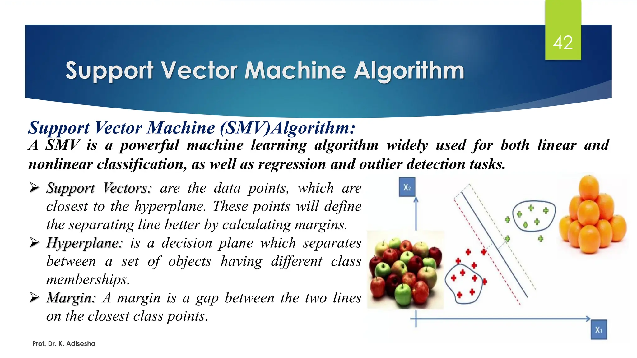
Support Vector Machine (SMV)Algorithm:
A SMV is a powerful machine learning algorithm widely used for both linear and
nonlinear classification, as well as regression and outlier detection tasks.
Prof. Dr. K. Adisesha
➢ Support Vectors: are the data points, which are
closest to the hyperplane. These points will define
the separating line better by calculating margins.
➢ Hyperplane: is a decision plane which separates
between a set of objects having different class
memberships.
➢ Margin: A margin is a gap between the two lines
on the closest class points.
43.
Support Vector MachineAlgorithm
43
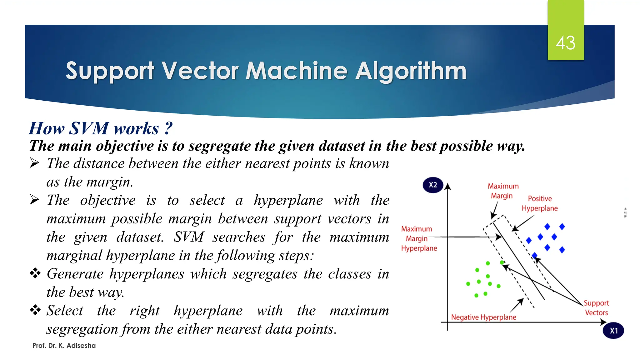
How SVM works ?
The main objective is to segregate the given dataset in the best possible way.
Prof. Dr. K. Adisesha
➢ The distance between the either nearest points is known
as the margin.
➢ The objective is to select a hyperplane with the
maximum possible margin between support vectors in
the given dataset. SVM searches for the maximum
marginal hyperplane in the following steps:
❖ Generate hyperplanes which segregates the classes in
the best way.
❖ Select the right hyperplane with the maximum
segregation from the either nearest data points.
44.
Support Vector MachineAlgorithm
44
How SVM works ?
The steps for using a Support Vector Machine (SVM) algorithm are:
Prof. Dr. K. Adisesha
➢ Import the data: Load the data set into the environment
➢ Explore the data: Understand what the data looks like
➢ Pre-process the data: Clean the data by handling missing values, outliers, and categorical
variables
➢ Split the data: Divide the data into training and testing sets
➢ Train the SVM: Use the training set to train the SVM algorithm
➢ Make predictions: Use the trained SVM to predict the class label for new data points
➢ Evaluate the results: Assess the performance of the SVM algorithm
45.
Support Vector MachineAlgorithm
45
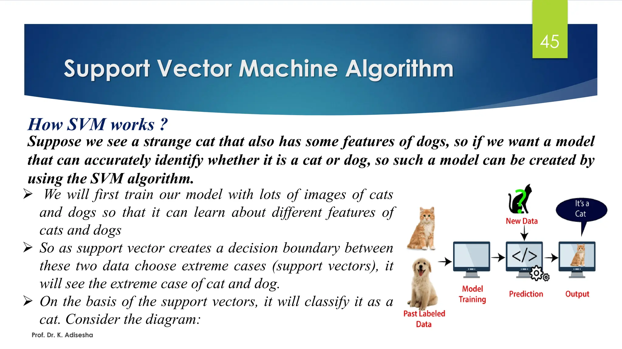
How SVM works ?
Suppose we see a strange cat that also has some features of dogs, so if we want a model
that can accurately identify whether it is a cat or dog, so such a model can be created by
using the SVM algorithm.
Prof. Dr. K. Adisesha
➢ We will first train our model with lots of images of cats
and dogs so that it can learn about different features of
cats and dogs
➢ So as support vector creates a decision boundary between
these two data choose extreme cases (support vectors), it
will see the extreme case of cat and dog.
➢ On the basis of the support vectors, it will classify it as a
cat. Consider the diagram:
46.
Support Vector MachineAlgorithm
46
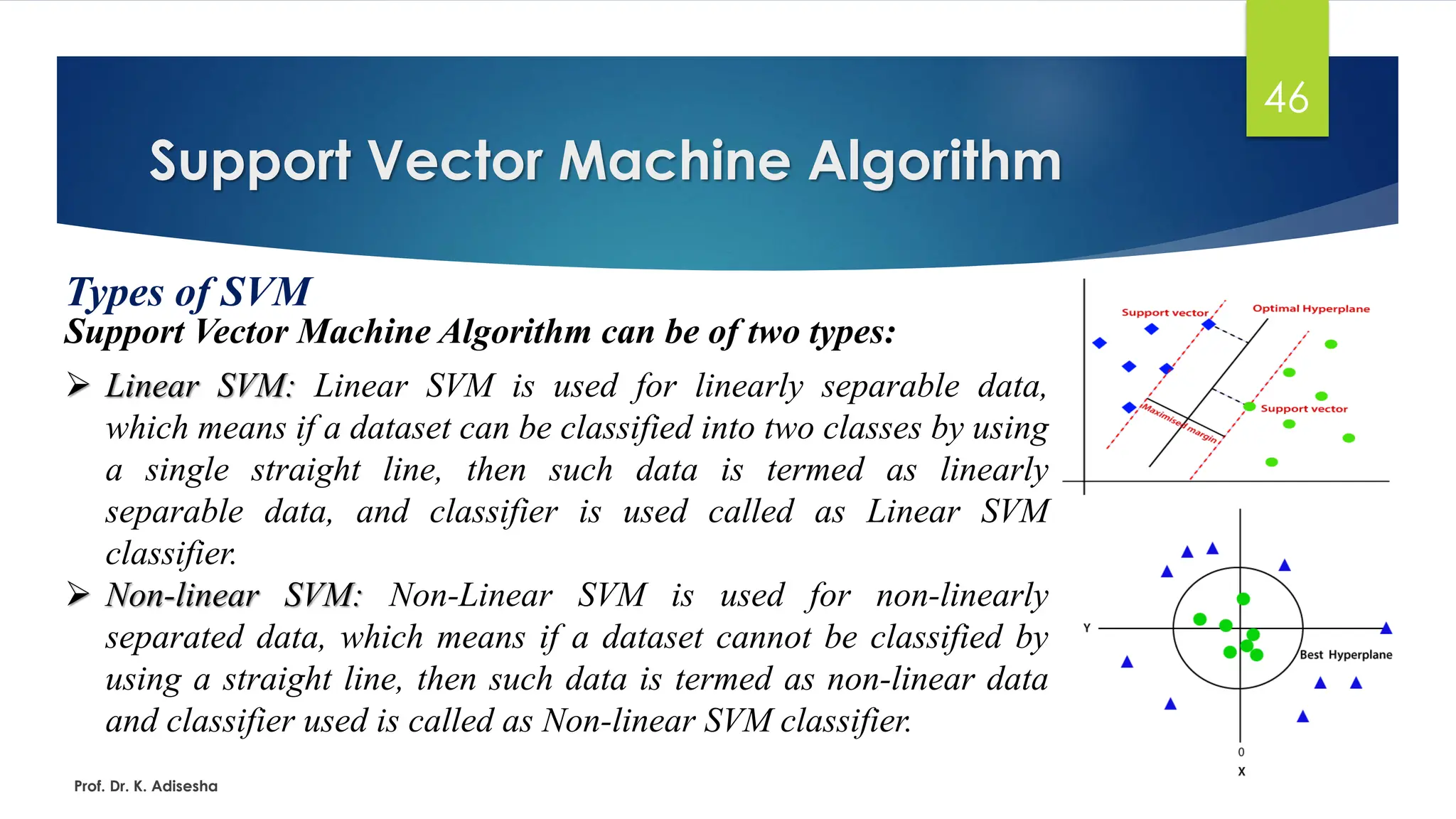
Types of SVM
Support Vector Machine Algorithm can be of two types:
Prof. Dr. K. Adisesha
➢ Linear SVM: Linear SVM is used for linearly separable data,
which means if a dataset can be classified into two classes by using
a single straight line, then such data is termed as linearly
separable data, and classifier is used called as Linear SVM
classifier.
➢ Non-linear SVM: Non-Linear SVM is used for non-linearly
separated data, which means if a dataset cannot be classified by
using a straight line, then such data is termed as non-linear data
and classifier used is called as Non-linear SVM classifier.
47.
Support Vector MachineAlgorithm
47
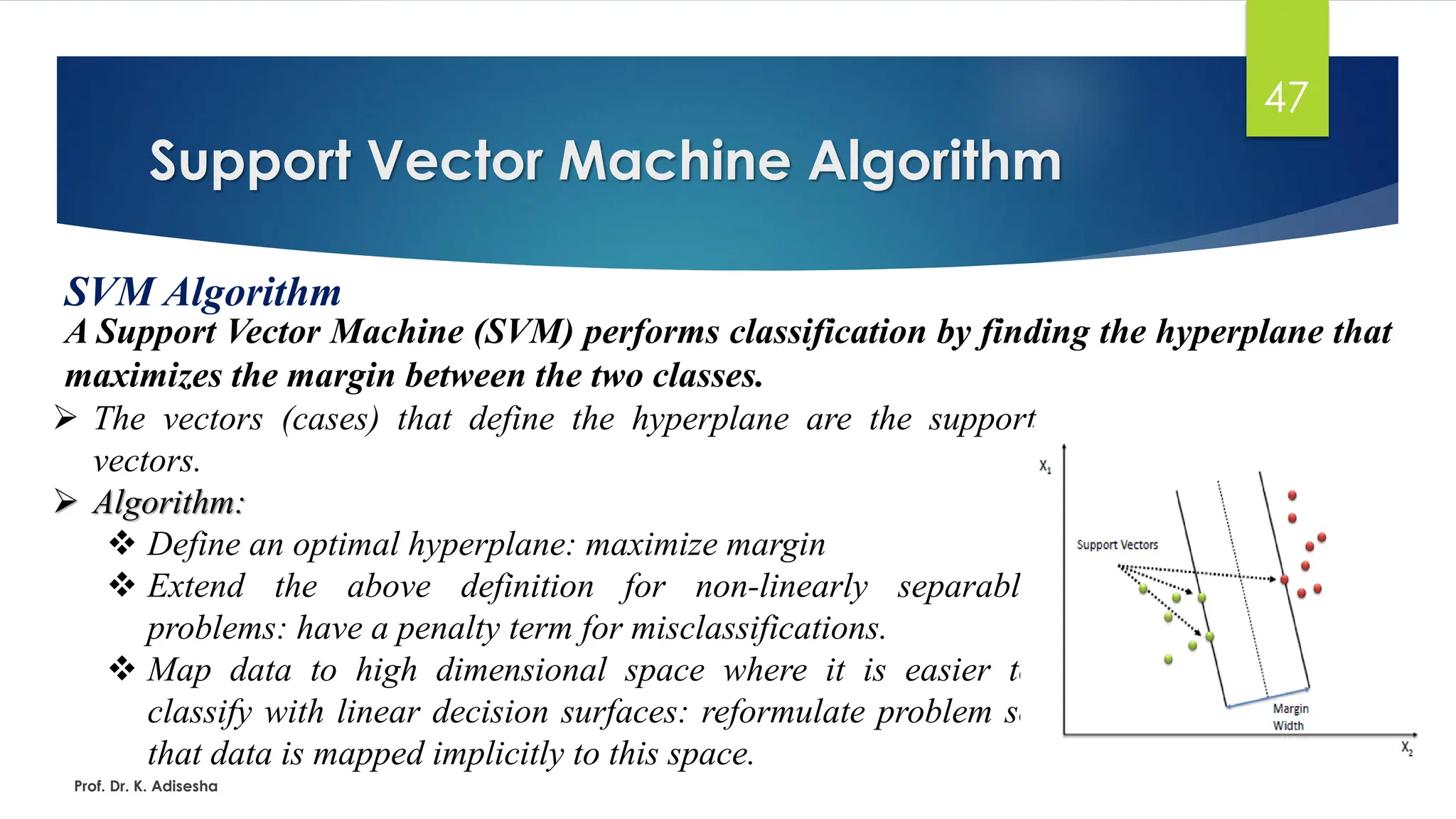
SVM Algorithm
A Support Vector Machine (SVM) performs classification by finding the hyperplane that
maximizes the margin between the two classes.
Prof. Dr. K. Adisesha
➢ The vectors (cases) that define the hyperplane are the support
vectors.
➢ Algorithm:
❖ Define an optimal hyperplane: maximize margin
❖ Extend the above definition for non-linearly separable
problems: have a penalty term for misclassifications.
❖ Map data to high dimensional space where it is easier to
classify with linear decision surfaces: reformulate problem so
that data is mapped implicitly to this space.
48.
Support Vector MachineAlgorithm
48
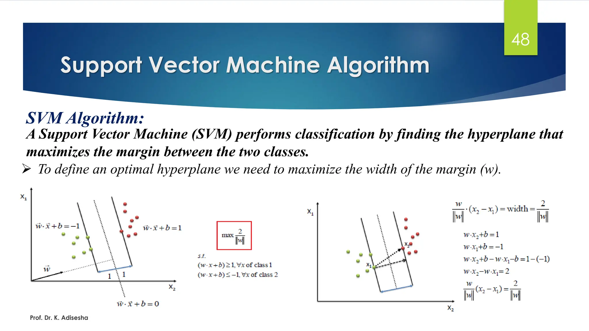
SVM Algorithm:
A Support Vector Machine (SVM) performs classification by finding the hyperplane that
maximizes the margin between the two classes.
Prof. Dr. K. Adisesha
➢ To define an optimal hyperplane we need to maximize the width of the margin (w).
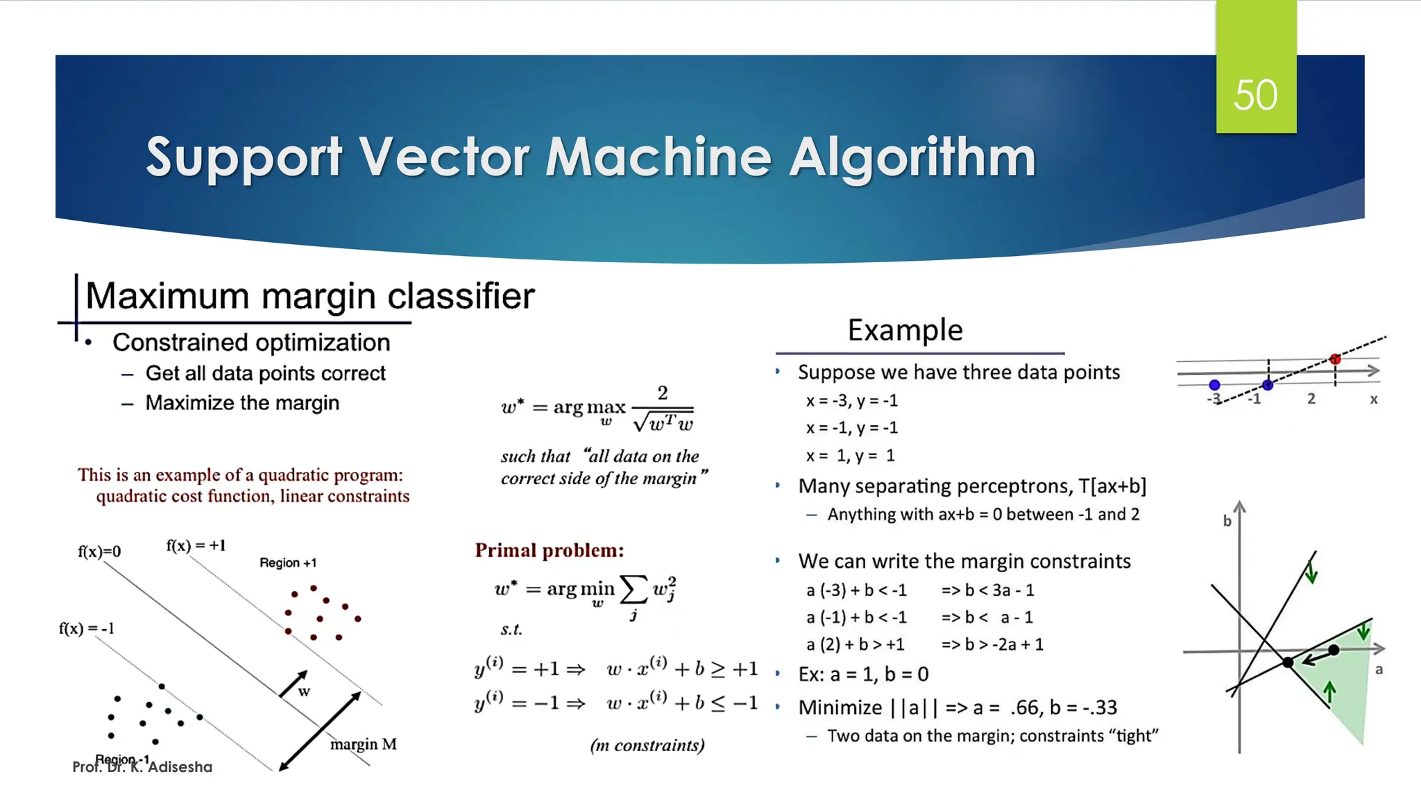
49.
Support Vector MachineAlgorithm
49
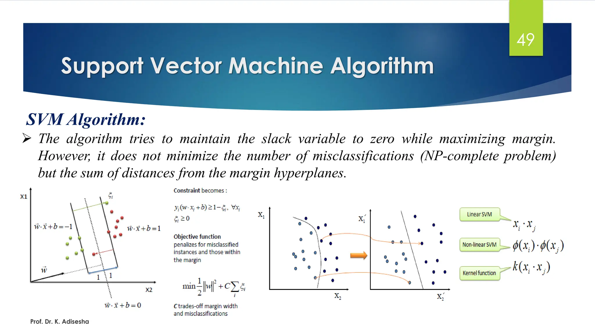
SVM Algorithm:
Prof. Dr. K. Adisesha
➢ The algorithm tries to maintain the slack variable to zero while maximizing margin.
However, it does not minimize the number of misclassifications (NP-complete problem)
but the sum of distances from the margin hyperplanes.