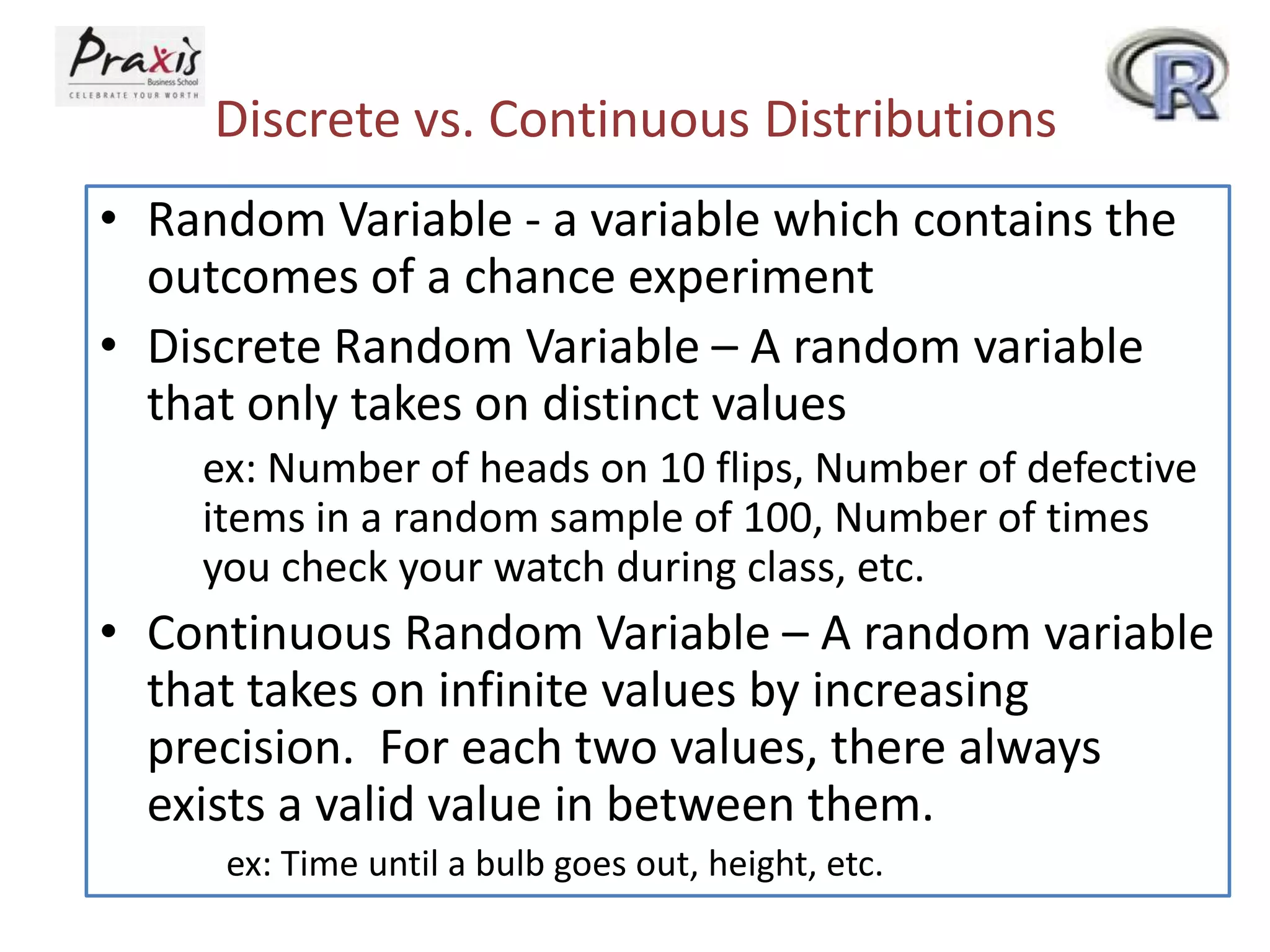
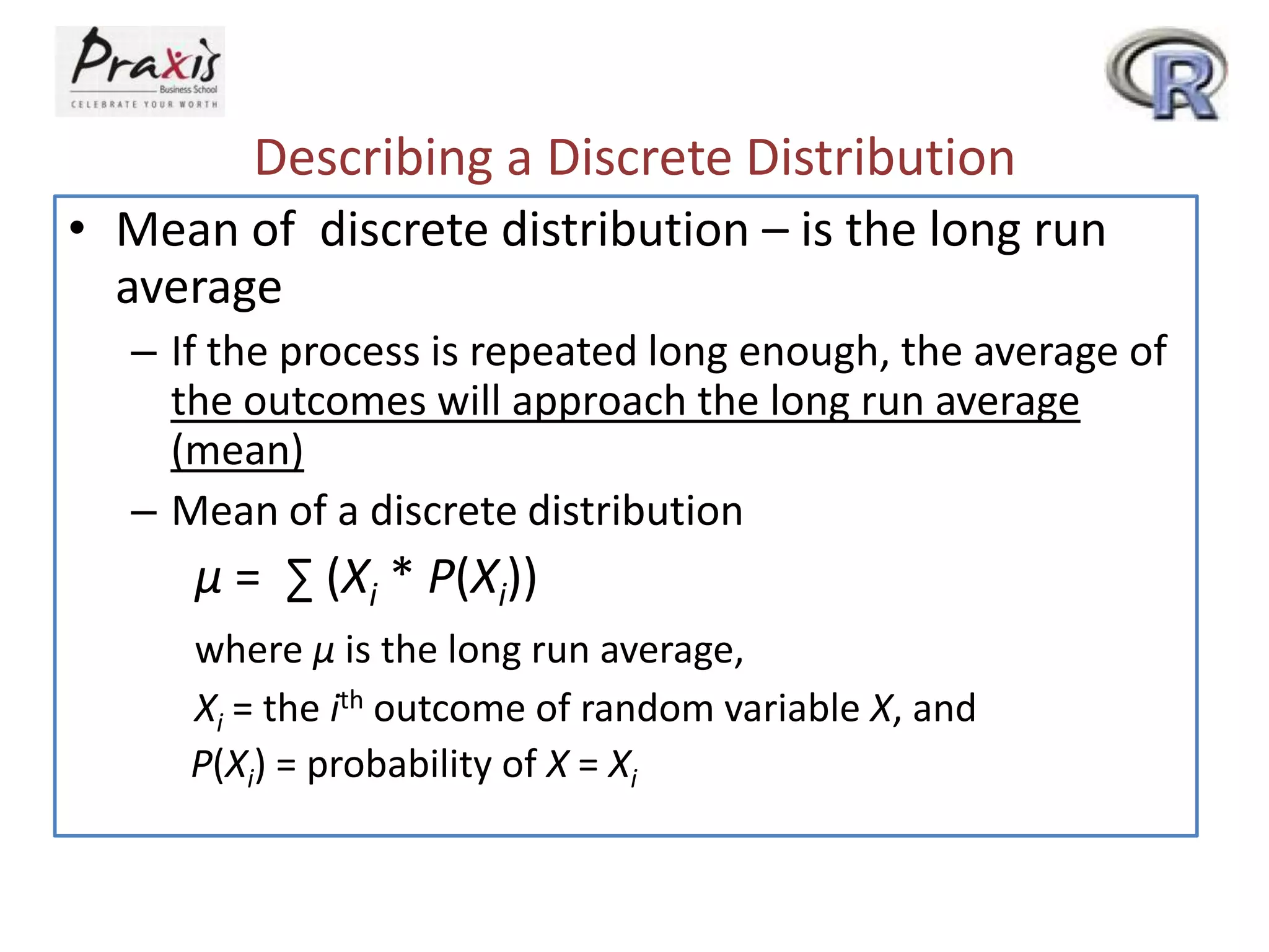
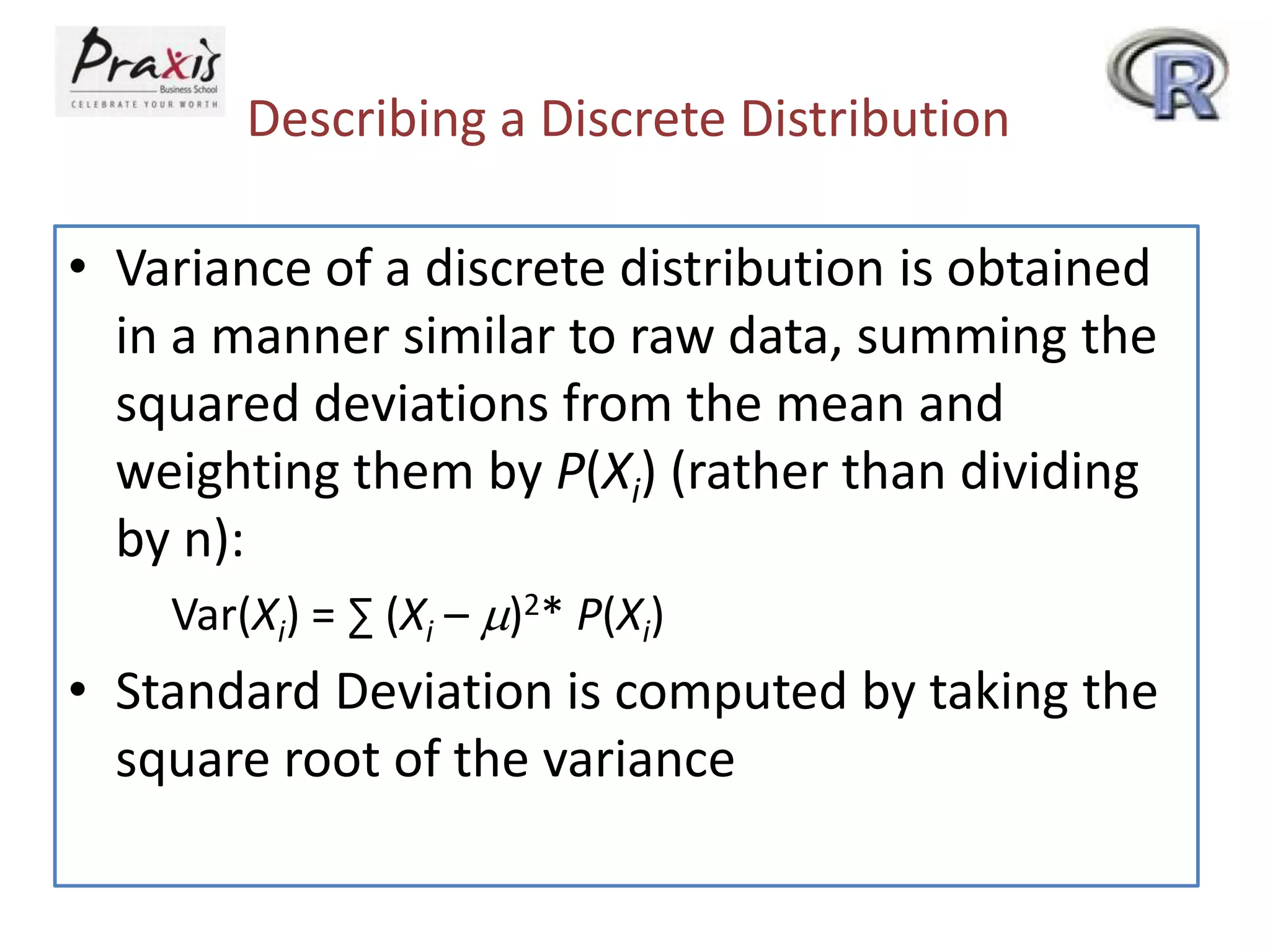
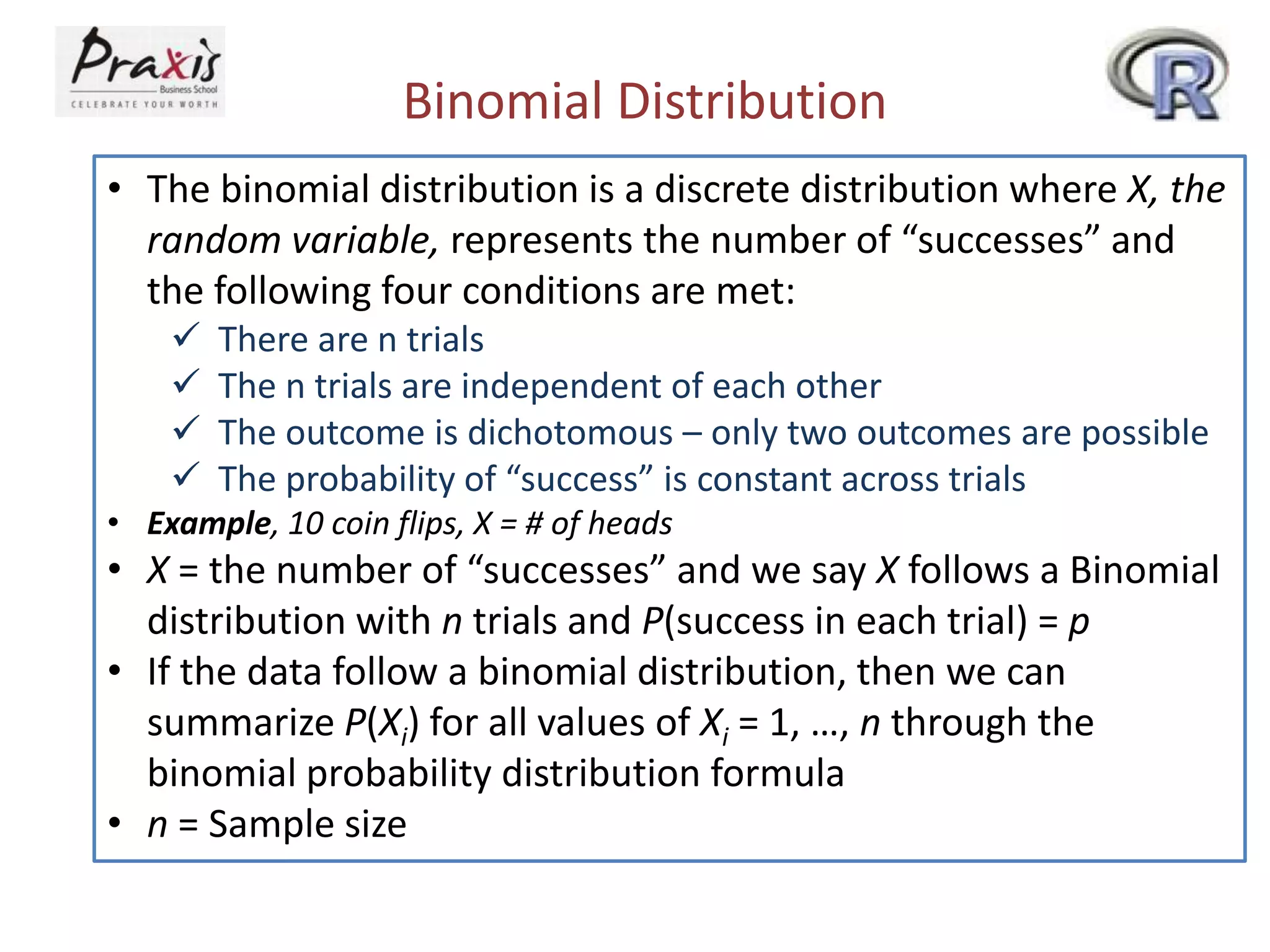
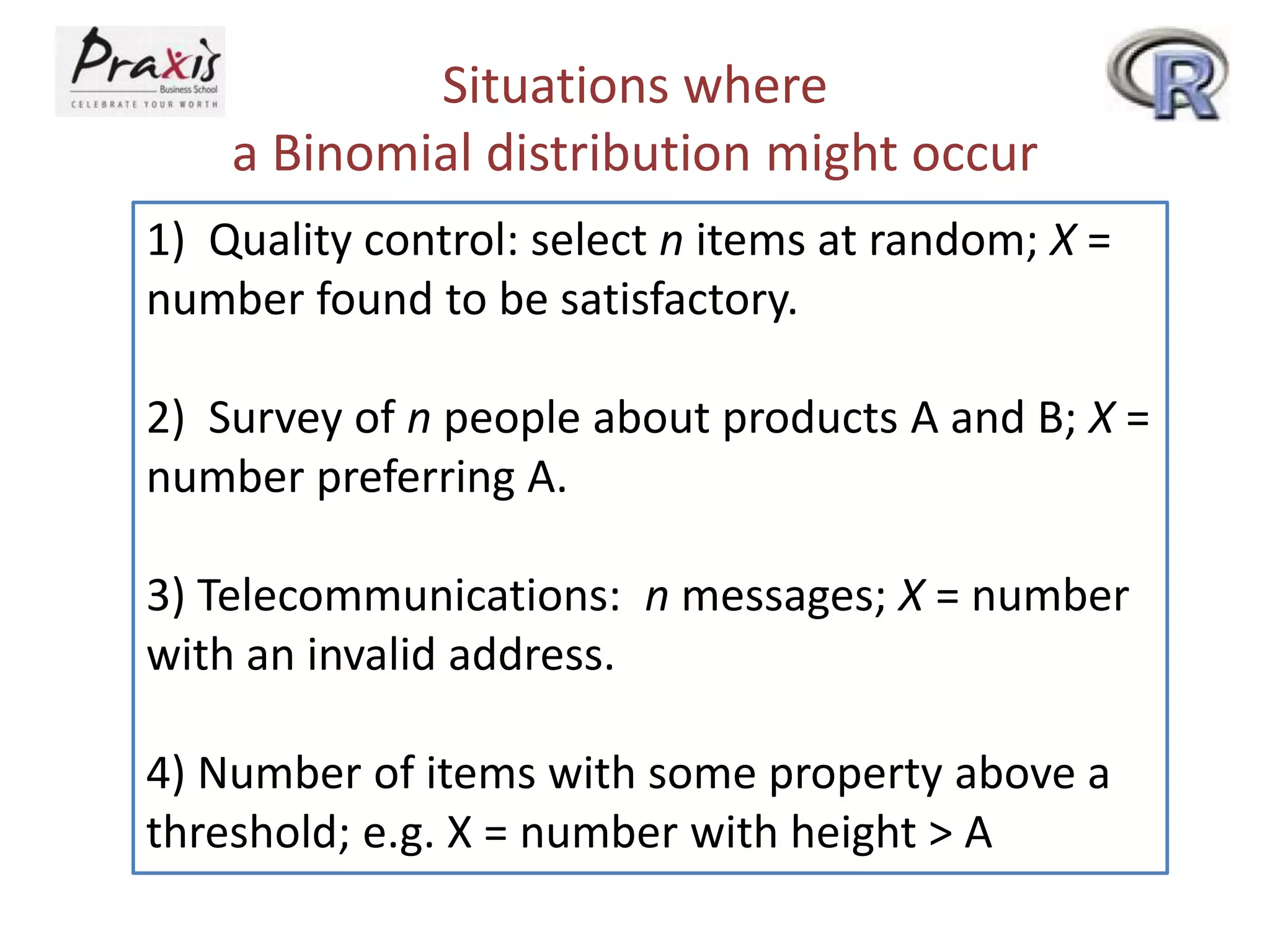
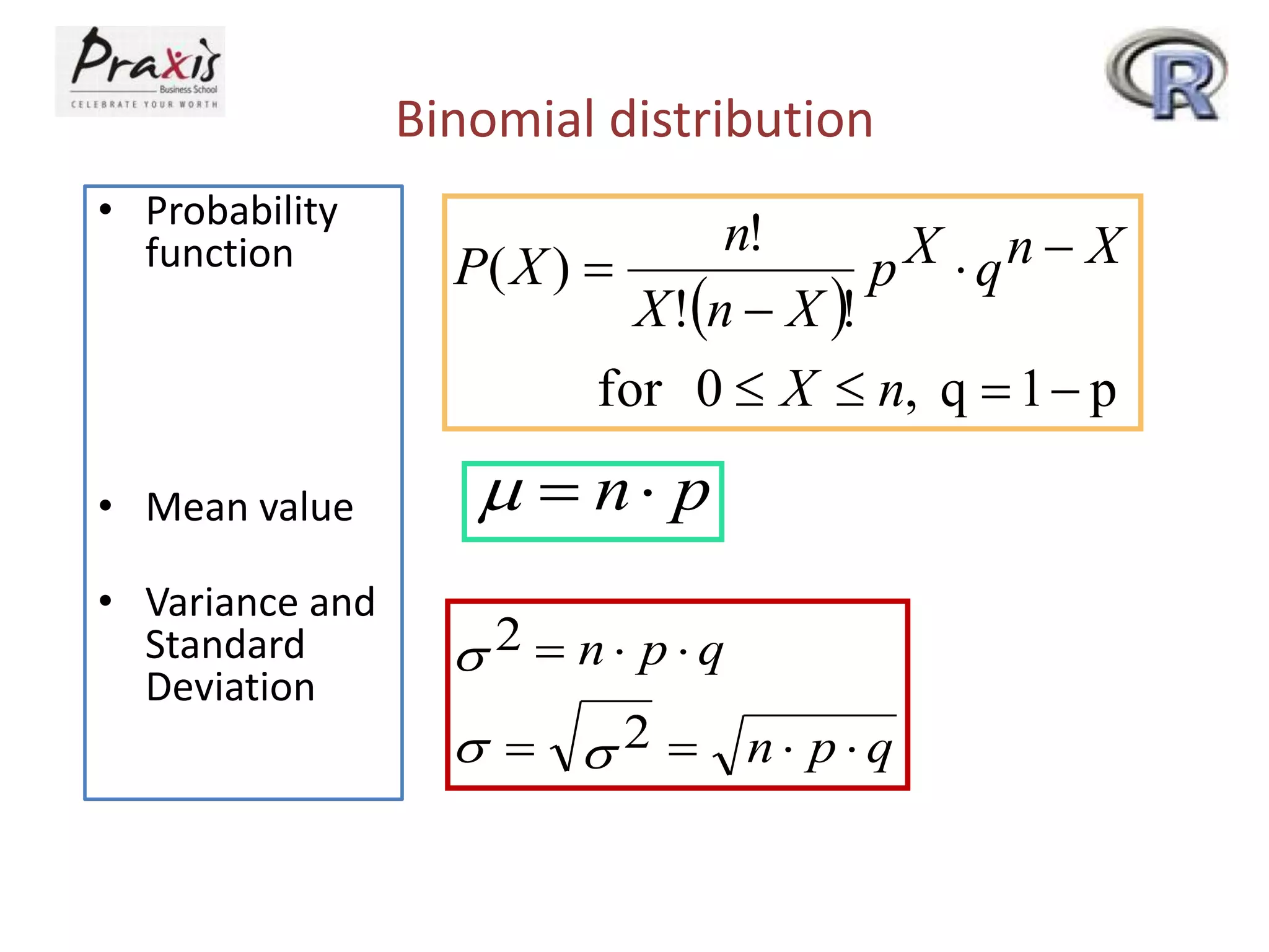
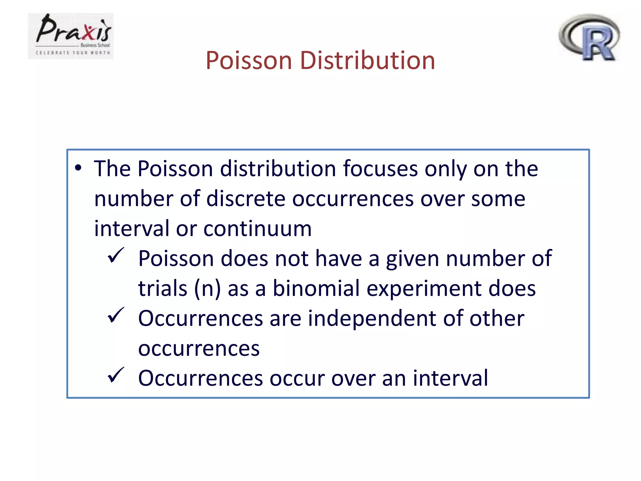
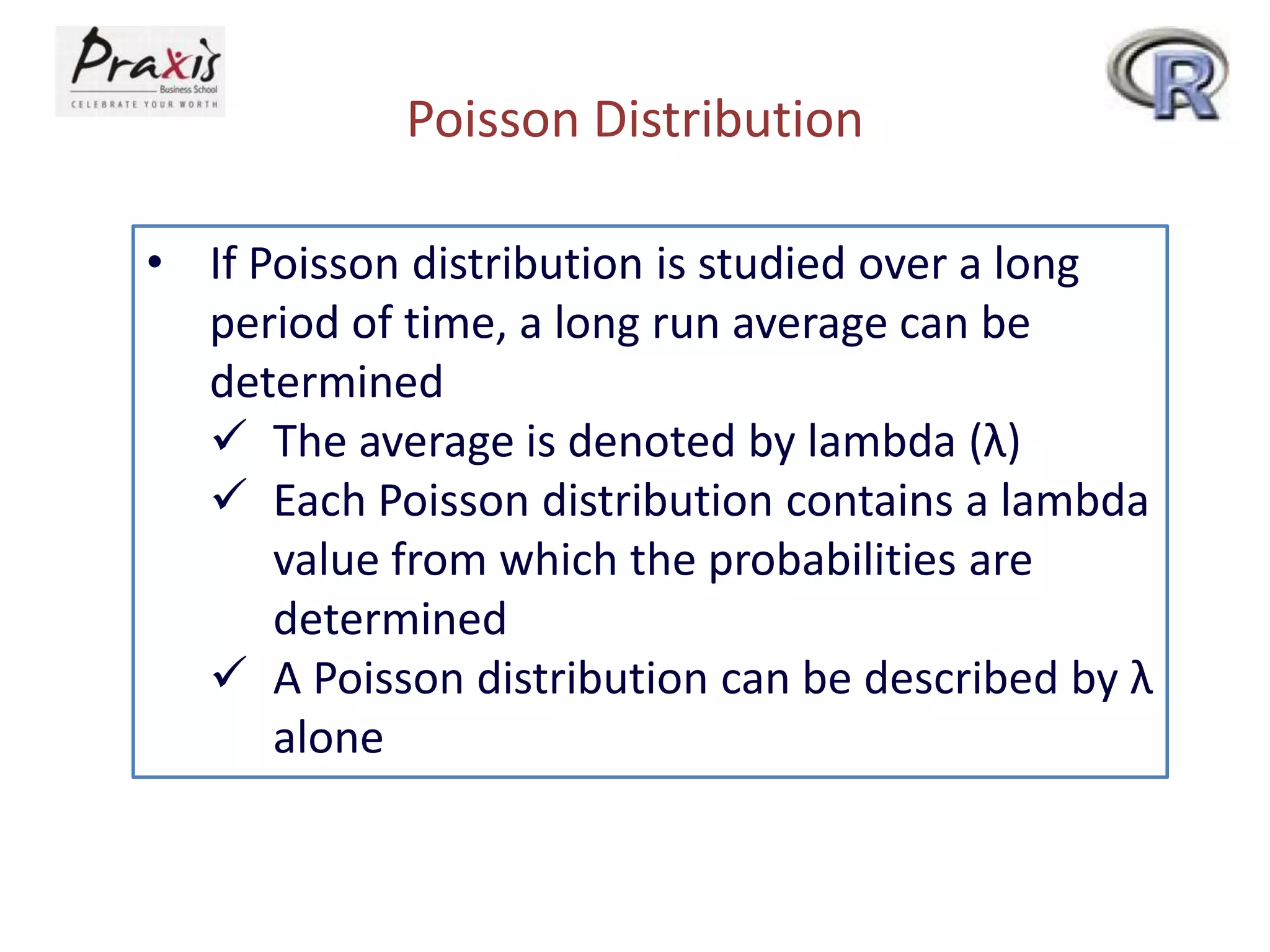
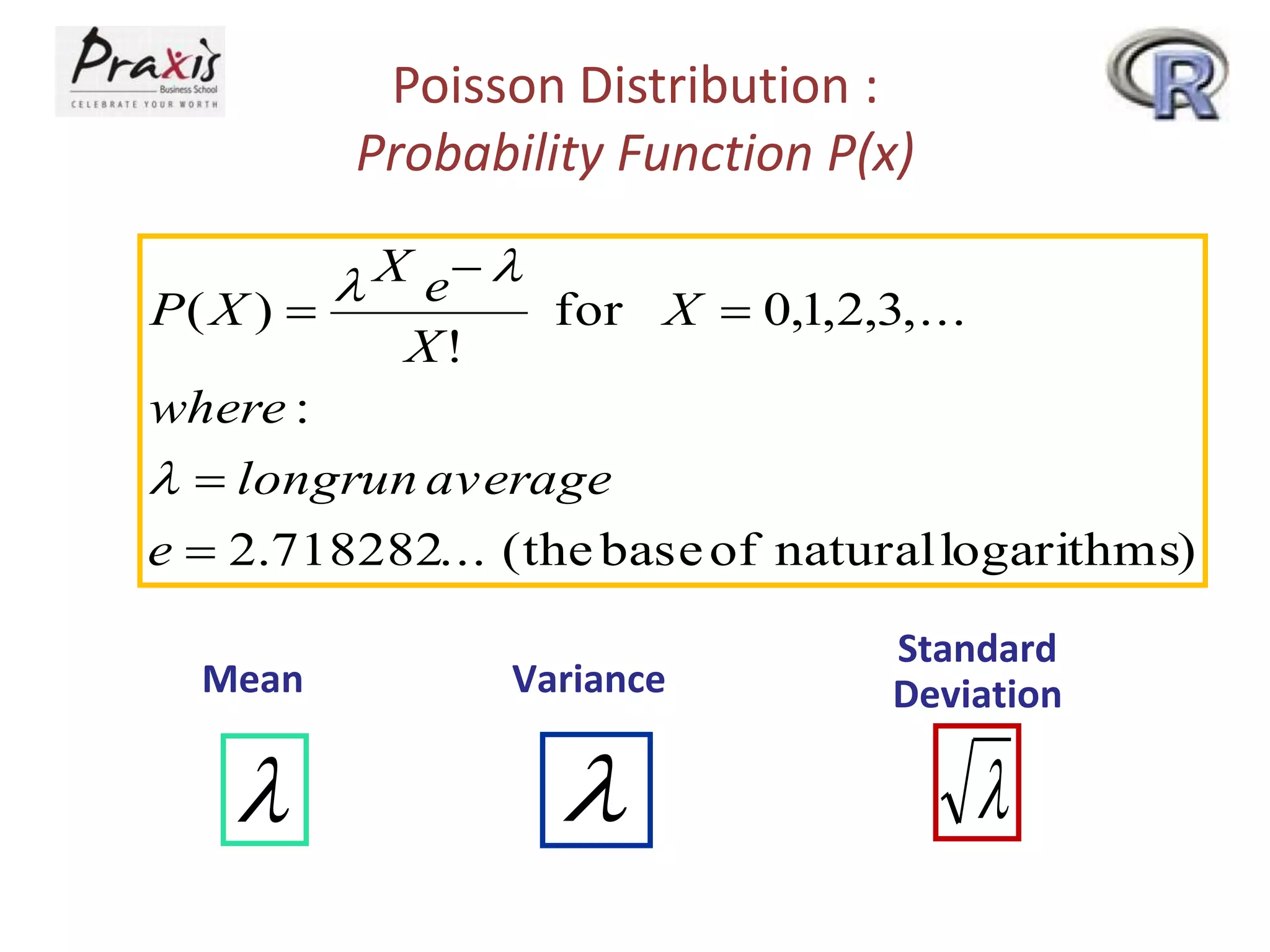
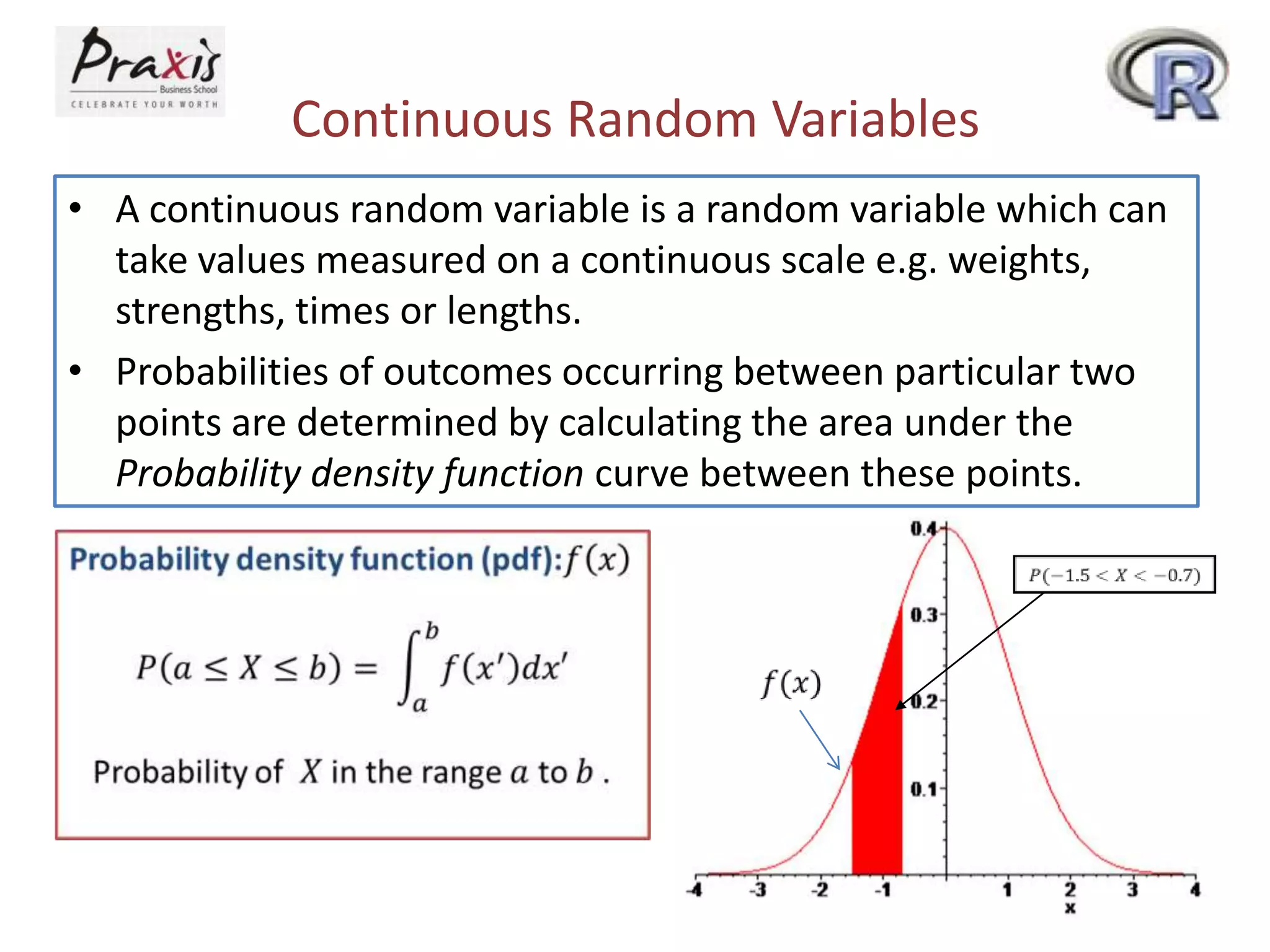
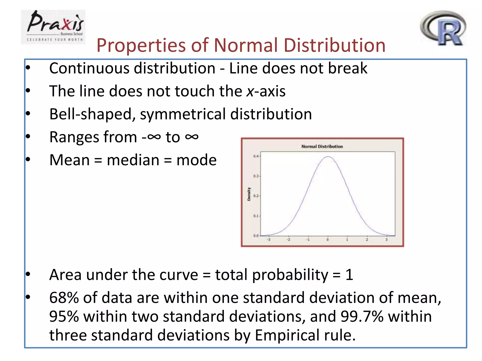
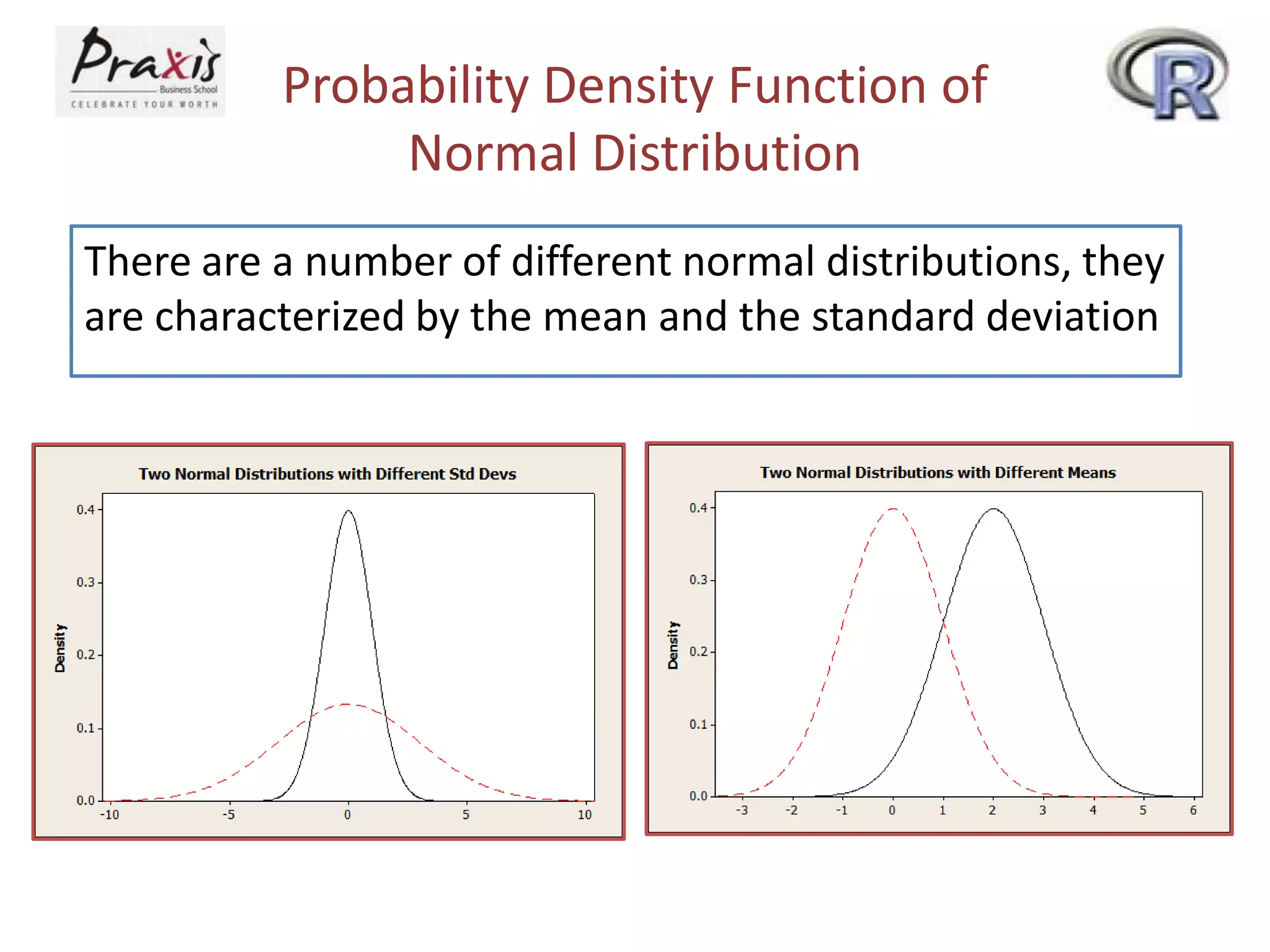
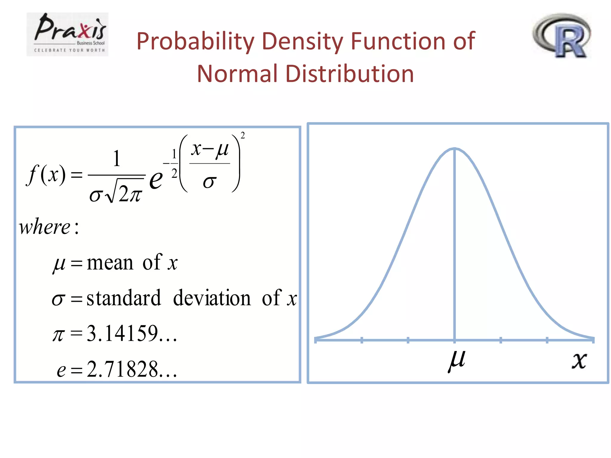
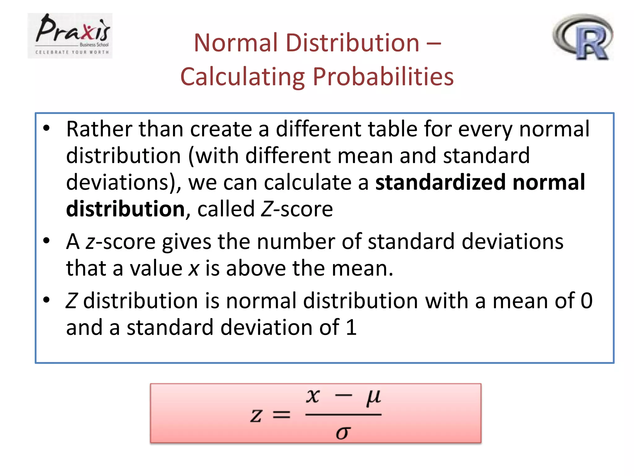
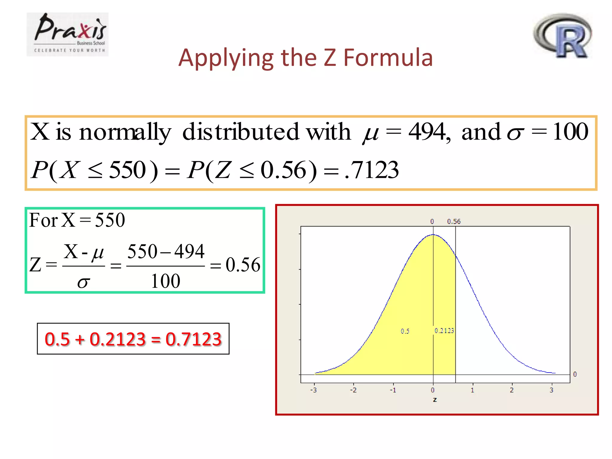
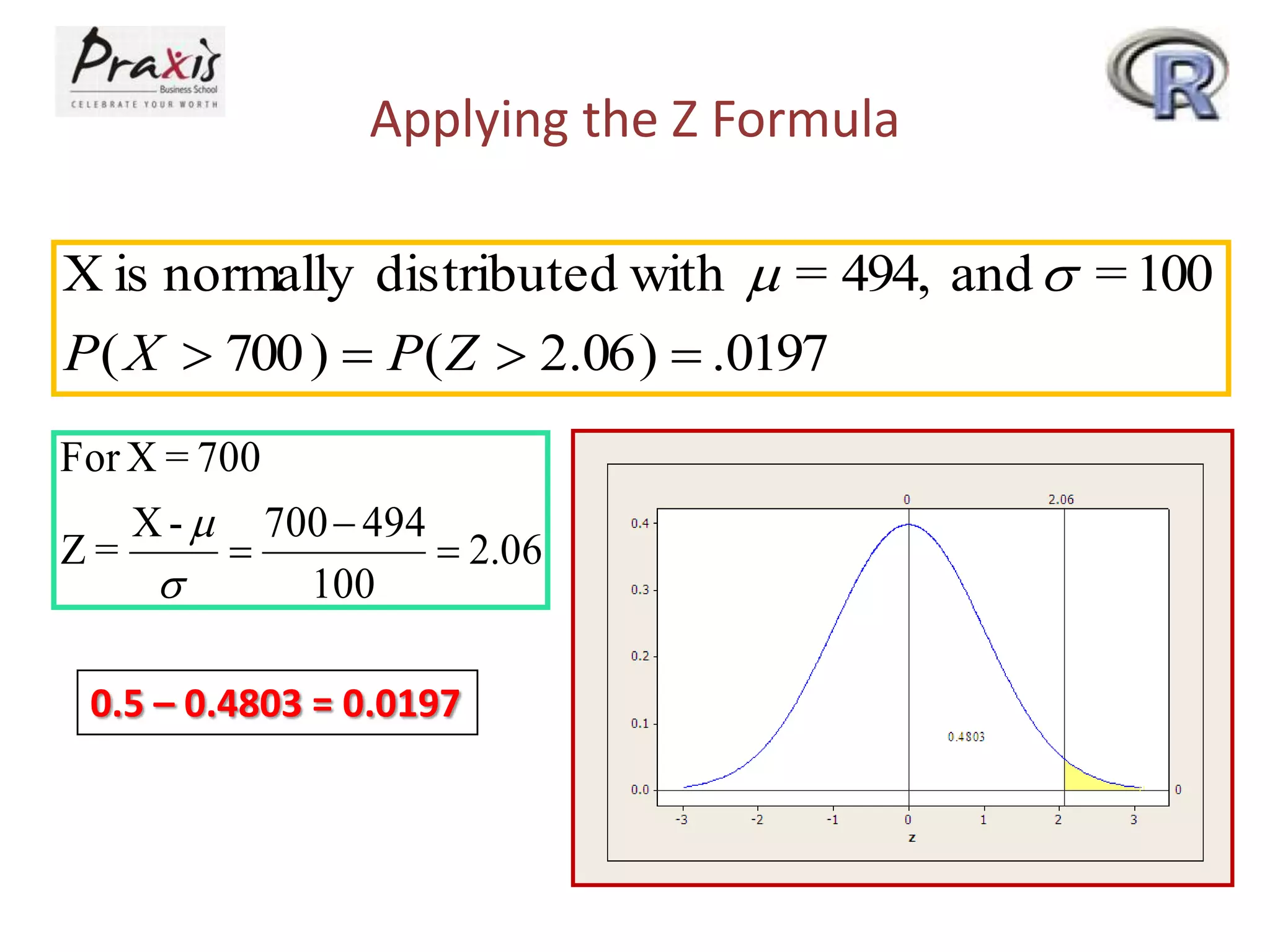
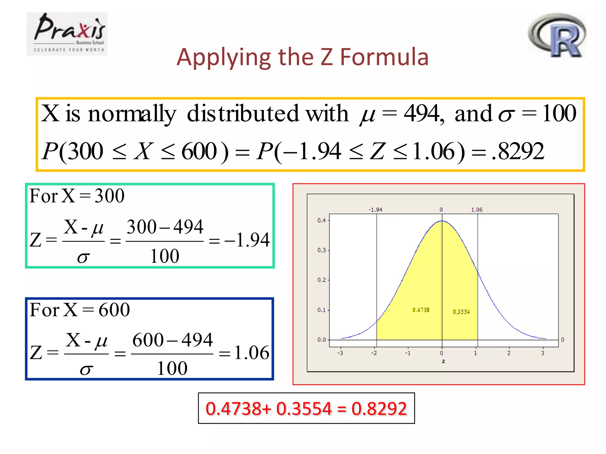
This document provides information about discrete and continuous probability distributions. It defines discrete and continuous random variables and gives examples of each. It describes how to calculate the mean and variance of discrete distributions. It also introduces the binomial, Poisson, and normal distributions and provides the key properties and formulas to describe and calculate probabilities for each distribution.

1. Discrete Distributions
• What is a random variable?
• Distinguish between discrete random variables
and continuous random variables.
• Know how to determine the mean and variance
of a discrete distribution.
• Identify the type of statistical experiments that
can be described by the binomial distribution,
and know how to calculate probabilities based on
the binomial distribution.

2. Discrete vs. Continuous Distributions
• Random Variable - a variable which contains the
outcomes of a chance experiment
• Discrete Random Variable – A random variable
that only takes on distinct values
ex: Number of heads on 10 flips, Number of defective
items in a random sample of 100, Number of times
you check your watch during class, etc.
• Continuous Random Variable – A random variable
that takes on infinite values by increasing
precision. For each two values, there always
exists a valid value in between them.
ex: Time until a bulb goes out, height, etc.

3. Describing a Distribution
• A distribution can be described by
constructing a graph of the distribution
• Measures of central tendency and variability
can be applied to distributions

4. Describing a Discrete Distribution
• Mean of discrete distribution – is the long run
average
– If the process is repeated long enough, the average of
the outcomes will approach the long run average
(mean)
– Mean of a discrete distribution
µ = ∑ (Xi * P(Xi))
where µ is the long run average,
Xi = the ith outcome of random variable X, and
P(Xi) = probability of X = Xi

5. Describing a Discrete Distribution
• Variance of a discrete distribution is obtained
in a manner similar to raw data, summing the
squared deviations from the mean and
weighting them by P(Xi) (rather than dividing
by n):
Var(Xi) = ∑ (Xi – m)2* P(Xi)
• Standard Deviation is computed by taking the
square root of the variance

6. Discrete Distribution -- Example
• An executive is considering out-of-town business travel
for a given Friday. At least one crisis could occur on the
day that the executive is gone. The distribution on the
following slide contains the number of crises that could
occur during the day the executive is gone and the
probability that each number will occur. For example,
there is a 0.37 probability that no crisis will occur, a 0.31
probability of one crisis, and so on.

7. Discrete Distribution -- Example
Distribution of Daily Crises
Number of
Crises ( X )
0
1
2
3
4
5
Probability
P(Xi)
0.37
0.31
0.18
0.09
0.04
0.01
P
r
o
b
a
b
i
l
i
t
y
P(Xi)
0.5
0.4
0.3
0.2
0.1
0
0
1
2
3
4
Number of Crises ( X )
5

8. Requirements for a Discrete
Probability Function -- Examples
• Each probability must be between 0 and 1
• The sum of all probabilities must be equal to 1.
X
P(X)
X
P(X)
X
P(X)
-1
0
1
2
3
.1
.2
.4
.2
.1
1.0
-1
0
1
2
3
-.1
.3
.4
.3
.1
1.0
-1
0
1
2
3
.1
.3
.4
.3
.1
1.2
VALID
NOT
VALID
NOT
VALID

9. Roulette
A roulette wheel has 37 pockets.
£1 on a number returns £36 if it comes
up (i.e. your £1 back + £35 winnings).
Otherwise you lose your £1.
What is the expected winnings (in
pounds) on a £1 number bet?
1.
2.
3.
4.
5.
-1/36
-1/37
-2/37
-1/35
1/36

10. Roulette
A roulette wheel has 37 pockets.
£1 on a number returns £36 if it comes
up (i.e. your £1 back + £35 winnings).
Otherwise you lose your £1.
What is the expected winnings (in
pounds) on a £1 number bet?

11. Binomial Distribution
• The binomial distribution is a discrete distribution where X, the
random variable, represents the number of “successes” and
the following four conditions are met:




There are n trials
The n trials are independent of each other
The outcome is dichotomous – only two outcomes are possible
The probability of “success” is constant across trials
• Example, 10 coin flips, X = # of heads
• X = the number of “successes” and we say X follows a Binomial
distribution with n trials and P(success in each trial) = p
• If the data follow a binomial distribution, then we can
summarize P(Xi) for all values of Xi = 1, …, n through the
binomial probability distribution formula
• n = Sample size

12. Situations where
a Binomial distribution might occur
1) Quality control: select n items at random; X =
number found to be satisfactory.
2) Survey of n people about products A and B; X =
number preferring A.
3) Telecommunications: n messages; X = number
with an invalid address.
4) Number of items with some property above a
threshold; e.g. X = number with height > A

13. Binomial distribution
• Probability
function
• Mean value
• Variance and
Standard
Deviation
n!
P( X ) 
p X  qn  X
X !n  X !
for 0  X  n, q  1  p
m  n p
 2  n pq
   2  n pq

14. Binomial Distribution:
Demonstration Problem 5.3
According to the U.S. Census Bureau,
approximately 6% of all workers in Jackson,
Mississippi, are unemployed. In conducting
a random telephone survey in Jackson,
what is the probability of getting two or
fewer unemployed workers in a sample of
20?

15. Binomial Distribution:
Demonstration Problem 5.3
According to the U.S. Census Bureau, approximately 6% of all workers
in Jackson, Mississippi, are unemployed. In conducting a random
telephone survey in Jackson, what is the probability of getting two or
fewer unemployed workers in a sample of 20?
• In this example,
– 6% are unemployed => p
– The sample size is 20 => n
– 94% are employed => q
– X is the number of successes desired
– What is the probability of getting 2 or fewer unemployed
workers in the sample of 20? => P(X≤2)
– The hard part of this problem is identifying p, n, and x

16. Binomial Distribution Table:
Demonstration Problem 5.3
According to the U.S. Census Bureau, approximately 6% of all workers in Jackson,
Mississippi, are unemployed. In conducting a random telephone survey in Jackson, what
is the probability of getting two or fewer unemployed workers in a sample of 20?
n = 20 PROBABILITY
X
0.05 0.06
0.07
0 0.3585 0.2901 0.2342
1 0.3774 0.3703 0.3526
2 0.1887 0.2246 0.2521
3 0.0596 0.0860 0.1139
4 0.0133 0.0233 0.0364
5 0.0022 0.0048 0.0088
6 0.0003 0.0008 0.0017
7 0.0000 0.0001 0.0002
8 0.0000 0.0000 0.0000
…
…
…
…
20 0.0000 0.0000 0.0000
n  20
p  .06
q  .94
P( X  2)  P( X  0)  P( X  1)  P( X  2)
 .2901 .3703  .2246  .8850

17. Poisson Distribution
• The Poisson distribution focuses only on the
number of discrete occurrences over some
interval or continuum
 Poisson does not have a given number of
trials (n) as a binomial experiment does
 Occurrences are independent of other
occurrences
 Occurrences occur over an interval

18. Poisson Distribution
• If Poisson distribution is studied over a long
period of time, a long run average can be
determined
 The average is denoted by lambda (λ)
 Each Poisson distribution contains a lambda
value from which the probabilities are
determined
 A Poisson distribution can be described by λ
alone

19. Poisson Distribution :
Probability Function P(x)
 X e   for X  0,1,2,3,...
P( X ) 
X!
where :
  longrun average
e  2.718282... (the base of natural logarithms)
Mean
Variance


Standard
Deviation


20. Continuous Random Variables
• A continuous random variable is a random variable which can
take values measured on a continuous scale e.g. weights,
strengths, times or lengths.
• Probabilities of outcomes occurring between particular two
points are determined by calculating the area under the
Probability density function curve between these points.

21. Properties of Normal Distribution
•
•
•
•
•
Continuous distribution - Line does not break
The line does not touch the x-axis
Bell-shaped, symmetrical distribution
Ranges from -∞ to ∞
Mean = median = mode
•
•
Area under the curve = total probability = 1
68% of data are within one standard deviation of mean,
95% within two standard deviations, and 99.7% within
three standard deviations by Empirical rule.

22. Probability Density Function of
Normal Distribution
There are a number of different normal distributions, they
are characterized by the mean and the standard deviation

23. Probability Density Function of
Normal Distribution
1 x m 
1
 

2
f ( x) 
e   
 2
where :
m  mean of x
  standard deviation of x
 = 3.14159. . .
e  2.71828. . .
2
m

24. Normal Distribution –
Calculating Probabilities
• Rather than create a different table for every normal
distribution (with different mean and standard
deviations), we can calculate a standardized normal
distribution, called Z-score
• A z-score gives the number of standard deviations
that a value x is above the mean.
• Z distribution is normal distribution with a mean of 0
and a standard deviation of 1

25. Standardized Normal Distribution –
Calculating Probabilities
• Z distribution probability values are given in table A5
of your book or can be calculated using software
• Table A5 gives the total area under the Z curve
between 0 and any point on the positive Z axis
• Since the curve is symmetric, the area under the
curve between Z and 0 is the same whether the Z
curve is positive or negative

26. Standardized Normal Distribution –
Calculating Probabilities – z table
Second Decimal Place in z
z 0.00
0.01
0.02
0.03
0.04
0.05
0.06
0.07
0.08
0.09
0.00
0.10
0.20
0.30
0.0000
0.0398
0.0793
0.1179
0.0040
0.0438
0.0832
0.1217
0.0080
0.0478
0.0871
0.1255
0.0120
0.0517
0.0910
0.1293
0.0160
0.0557
0.0948
0.1331
0.0199
0.0596
0.0987
0.1368
0.0239
0.0636
0.1026
0.1406
0.0279
0.0675
0.1064
0.1443
0.0319
0.0714
0.1103
0.1480
0.0359
0.0753
0.1141
0.1517
0.90
1.00
1.10
1.20
0.3159
0.3413
0.3643
0.3849
0.3186
0.3438
0.3665
0.3869
0.3212
0.3461
0.3686
0.3888
0.3238
0.3485
0.3708
0.3907
0.3264
0.3508
0.3729
0.3925
0.3289
0.3531
0.3749
0.3944
0.3315
0.3554
0.3770
0.3962
0.3340
0.3577
0.3790
0.3980
0.3365
0.3599
0.3810
0.3997
0.3389
0.3621
0.3830
0.4015
2.00
0.4772
0.4778
0.4783
0.4788
0.4793
0.4798
0.4803
0.4808
0.4812
0.4817
3.00
3.40
3.50
0.4987
0.4997
0.4998
0.4987
0.4997
0.4998
0.4987
0.4997
0.4998
0.4988
0.4997
0.4998
0.4988
0.4997
0.4998
0.4989
0.4997
0.4998
0.4989
0.4997
0.4998
0.4989
0.4997
0.4998
0.4990
0.4997
0.4998
0.4990
0.4998
0.4998

27. Table Lookup of a Standardized
Normal Probability
P(0  Z  1)  0. 3413
Z
0.00
0.01
0.02
0.00
0.10
0.20
1.00
-3
-2
-1
0
1
2
3
0.0000 0.0040 0.0080
0.0398 0.0438 0.0478
0.0793 0.0832 0.0871
0.3413 0.3438 0.3461
1.10
1.20
0.3643 0.3665 0.3686
0.3849 0.3869 0.3888

28. Applying the Z Formula
X is normally distributed withm = 485, and  = 105
P( 485  X  600)  P( 0  Z  1.10) . 3643
For X = 485,
X - m 485  485
Z=

0

105
For X = 600,
X - m 600  485
Z=

 1.10

105
Z
0.00
0.01
0.02
0.00
0.10
0.0000 0.0040 0.0080
0.0398 0.0438 0.0478
1.00
0.3413 0.3438 0.3461
1.10
0.3643 0.3665 0.3686
1.20
0.3849 0.3869 0.3888

29. Applying the Z Formula
X is normally distributed with m = 494, and  = 100
P( X  550 )  P( Z  0.56 )  .7123
For X = 550
X - m 550  494
Z=

 0.56

100
0.5 + 0.2123 = 0.7123

30. Applying the Z Formula
X is normally distributed with m = 494, and  = 100
P( X  700 )  P ( Z  2.06 )  .0197
For X = 700
Z=
X - m 700  494

 2.06

100
0.5 – 0.4803 = 0.0197

31. Applying the Z Formula
X is normally distributed with m = 494, and  = 100
P(300  X  600 )  P (1.94  Z  1.06 )  .8292
For X = 300
Z=
X-m

300  494

 1.94
100
For X = 600
Z=
X-m

600  494

 1.06
100
0.4738+ 0.3554 = 0.8292