Download to read offline


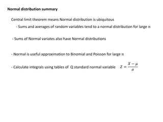
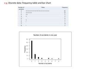

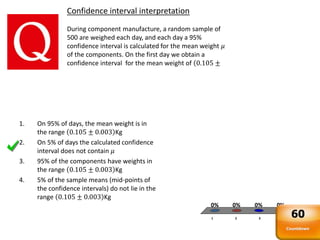
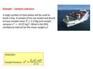
![Maximum likelihood estimator: the value of θ that maximizes the likelihood
𝑃(𝐷|𝜃) is called the maximum likelihood estimate: it is the value that makes the
data most likely, and if P(θ) does not depend on parameters (e.g. is a constant) is
also the most probable value of the parameter given the observed data.
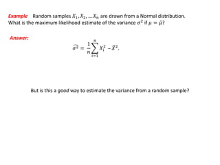
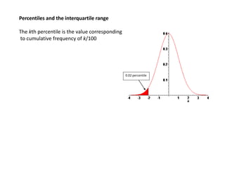
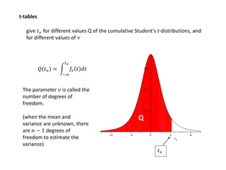
Example Random samples 𝑋1, 𝑋2, … 𝑋 𝑛 are drawn from a Normal distribution.
What is the maximum likelihood estimate of the mean μ?
𝜇 = 𝑋 =
1
𝑛
𝑖=1
𝑛
𝑋𝑖Answer: Sample mean:
𝑃(𝜇|𝐷)
𝜇
𝜇
[see notes]](https://image.slidesharecdn.com/statistics782-140528003145-phpapp02/85/Statistics78-2-23-320.jpg)
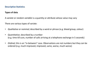
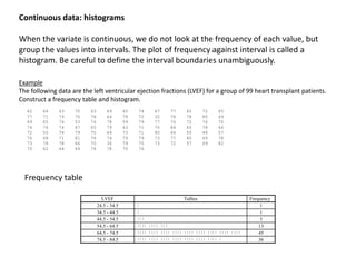
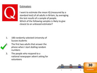
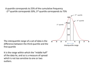
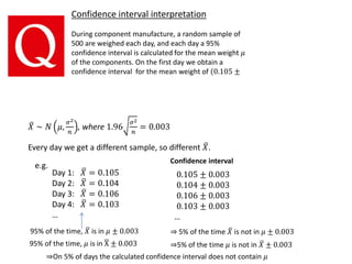
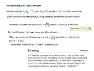
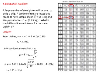
![A good but biased estimator
A poor but unbiased estimator
True mean
Comparing estimators
What are good properties of an estimator?
- Efficient: estimate close to true value with most sets of data random data samples
- Unbiased: on average (over possible data samples) it gives the true value
The estimator 𝜃 is unbiased for 𝜃 if 𝐸 𝜃 = 𝜃 for all values of 𝜃.
𝑃( 𝜃)
[distribution of
Maximum-
likelihood
𝜃 over all possible
random samples]](https://image.slidesharecdn.com/statistics782-140528003145-phpapp02/85/Statistics78-2-25-320.jpg)
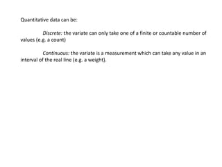
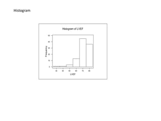
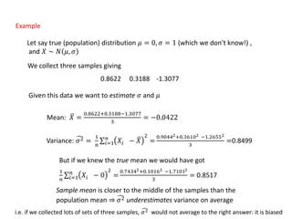
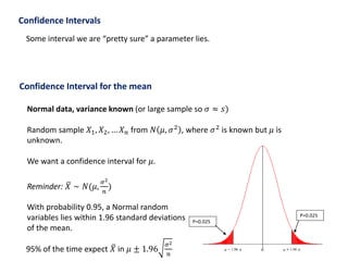
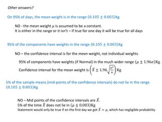
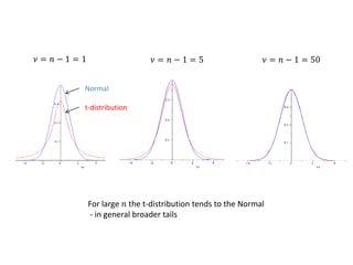
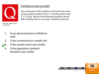
![Result: 𝜇 = 𝑋 is an unbiased estimator of 𝜇.
𝑋 =
1
𝑛
𝑋1 + ⋯ + 𝑋 𝑛 = 𝜇
Result: 𝜎2 is a biased estimator of σ2
𝜎2 =
𝑛 − 1
𝑛
𝜎2 [proof in notes]](https://image.slidesharecdn.com/statistics782-140528003145-phpapp02/85/Statistics78-2-27-320.jpg)


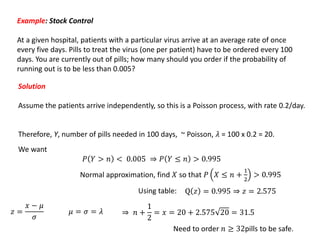
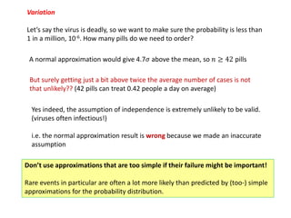
1. The document summarizes key concepts from a lecture on statistics for engineers, including the normal distribution, the central limit theorem, and normal approximations to the binomial and Poisson distributions. 2. It provides an example of using the normal approximation to the Poisson distribution to calculate how many pills should be ordered to ensure the probability of running out is less than 0.005. 3. The document cautions that normal approximations may provide inaccurate results if assumptions like independence are violated, as with infectious diseases. Simple approximations are not advisable if failure could have important consequences, as with estimating rare event probabilities.


![Lesson3 lpart one - Measures mean [Autosaved].pptx](https://cdn.slidesharecdn.com/ss_thumbnails/lesson2-measuresmeanautosaved-241011173812-613e1e66-thumbnail.jpg?width=640&height=640&fit=bounds)


