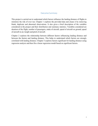
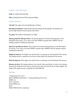
The project looks at factors which impact landing distance of a commercial flight so as to minimize risk over run. SAS is used to perform exploratory data analysis and fit a regression model.

1. Project Report
Statistical Computing
Rashmi Subrahmanya
University of Cincinnati

2. Contents
Executive Summary....................................................................................................................................i
Chapter 1: Data Preparation.....................................................................................................................1
Variable dictionary....................................................................................................................................1
SAS Code ...............................................................................................................................................1
SAS Output............................................................................................................................................4
Observations.........................................................................................................................................7
Conclusion.............................................................................................................................................8
Chapter 2: Descriptive Study ....................................................................................................................8
SAS Code ...............................................................................................................................................8
SAS Output............................................................................................................................................9
Observations.......................................................................................................................................11
Conclusion...........................................................................................................................................12
Chapter 3: Statistical Modeling...............................................................................................................12
SAS Code .............................................................................................................................................12
SAS Output..........................................................................................................................................13
Observations.......................................................................................................................................16
Conclusion...........................................................................................................................................17

3. i
Executive Summary
This project is carried out to understand which factors influence the landing distance of flights to
minimize the risk of over run. Chapter 1 explores the provided data and cleans it by removing
blank, duplicate and abnormal observations. It also gives a brief description of the variables
considered in the project and their distribution and summary statistics. Variables considered are
duration of the flight, number of passengers, make of aircraft, speed of aircraft on ground, speed
of aircraft in air, height and pitch of aircraft.
Chapter 2 explores the relationship between different factors influencing landing distance and
between the factors and landing distance. This helps to understand which factors are strongly
correlated with landing distance. Chapter 3 explores factors significant for landing distance using
regression analysis and then fits a linear regression model based on significant factors.

4. 1
Chapter 1: Data Preparation
Goal: To explore and clean data
Data: Landing data from 950 commercial flights
Variable dictionary
Aircraft: The make of an aircraft (Boeing or Airbus).
Duration (in minutes): Flight duration between taking off and landing. The duration of a
normal flight should always be greater than 40min.
No_pasg: The number of passengers in a flight.
Speed_ground (in miles per hour): The ground speed of an aircraft when passing over the
threshold of the runway. If its value is less than 30MPH or greater than 140MPH, then the
landing would be considered as abnormal.
Speed_air (in miles per hour): The air speed of an aircraft when passing over the threshold of
the runway. If its value is less than 30MPH or greater than 140MPH, then the landing would be
considered as abnormal.
Height (in meters): The height of an aircraft when it is passing over the threshold of the runway.
The landing aircraft is required to be at least 6 meters high at the threshold of the runway.
Pitch (in degrees): Pitch angle of an aircraft when it is passing over the threshold of the runway.
Distance (in feet): The landing distance of an aircraft. More specifically, it refers to the distance
between the threshold of the runway and the point where the aircraft can be fully stopped. The
length of the airport runway is typically less than 6000 feet.
SAS Code
/**Importing FAA1.xls**/
PROC IMPORT DATAFILE="~/Classwork/Project/FAA1.xls"
DBMS=xls
OUT=work.faa1;
GETNAMES=yes;
RUN;
PROC PRINT DATA=work.faa1;

5. 2
RUN;
/**Importing FAA2.xls**/
PROC IMPORT DATAFILE="~/Classwork/Project/FAA2.xls"
DBMS=xls
OUT=work.faa2;
GETNAMES=yes;
RUN;
PROC PRINT DATA=work.faa2;
RUN;
/**Deleting blank rows which were imported in FAA2.xls**/
DATA faa2;
SET faa2;
IF aircraft='' THEN DELETE;
RUN;
PROC PRINT DATA=faa2;
RUN;
/**Combining two data sets by concatenation**/
DATA combined;
SET faa1 faa2;
RUN;
PROC PRINT DATA=combined;
RUN;
/**Checking for Duplicate Rows**/
PROC SORT DATA=combined OUT=sorted NODUPKEY;
BY speed_ground;
RUN;
PROC PRINT DATA=sorted;
RUN;
/** Checking for missing values**/
PROC SORT DATA=sorted OUT=sorted;
BY aircraft;
RUN;
PROC MEANS DATA=sorted N NMISS MEAN RANGE;
VAR duration no_pasg speed_ground speed_air height pitch distance;
RUN;

6. 3
/**Checking for abnormal values**/
DATA validation;
SET sorted;
IF duration>=40 THEN normal_duration='YES';
ELSE IF duration = ' ' THEN normal_duration=' ';
ELSE normal_duration='NO';
IF speed_ground>=30 AND speed_ground<=140 THEN normal_speed_ground='YES';
ELSE normal_speed_ground='NO';
IF speed_air>=30 AND speed_air<=140 THEN normal_speed_air='YES';
ELSE IF speed_air=' ' THEN normal_speed_air=' ';
ELSE normal_speed_air='NO';
IF height>=6 THEN normal_height='YES';
ELSE normal_height='NO';
IF distance<6000 THEN normal_distance='YES';
ELSE normal_distance='NO';
RUN;
PROC PRINT DATA=validation;
RUN;
/**Counting abnormal values**/
PROC FREQ DATA=validation;
TABLE normal_duration normal_speed_ground normal_speed_air normal_height
normal_distance;
RUN;
/**Since number of observations with abnormal values is low, they are deleted**/
DATA combined_new;
SET validation;
IF normal_duration='NO' THEN DELETE;
IF normal_speed_ground='NO' THEN DELETE;
IF normal_speed_air='NO' THEN DELETE;
IF normal_height='NO' THEN DELETE;
IF normal_distance='NO' THEN DELETE;
RUN;
PROC PRINT DATA=combined_new;
RUN;
/**Summarizing the distribution of each variable**/
PROC UNIVARIATE DATA=combined_new;

7. 4
VAR duration no_pasg speed_ground speed_air height pitch distance;
RUN;
/**Summary statistics of cleaned data**/
PROC MEANS DATA=combined_new;
VAR duration no_pasg speed_ground speed_air height pitch distance;
RUN;
/**Renaming the data set**/
DATA flight;
SET combined_new;
RUN;
SAS Output
Figure 1: Checking for missing values in the combined data set

8. 5
Figure 2: Checking for number of abnormal values in the variables
Figure 3: Distribution of duration Figure 4: Distribution of no_pasg
40 60 80 100 120 140 160 180 200 220 240 260 280 300
duration
0
5
10
15
20
Percent
Distributionof duration
30 34 38 42 46 50 54 58 62 66 70 74 78 82 86
no_pasg
0
5
10
15
20
25
Percent
Distributionof no_pasg

9. 6
Figure 5: Distribution of speed_ground Figure 6: Distribution of speed_air
Figure 7:Distribution of height Figure 8: Distribution of pitch
Figure 9: Distribution of distance
36 44 52 60 68 76 84 92 100 108 116 124 132
speed_ground
0
5
10
15
20
Percent Distributionof speed_ground
92.5 97.5 102.5 107.5 112.5 117.5 122.5 127.5 132.5
speed_air
0
5
10
15
20
25
30
Percent
Distributionof speed_air
8 12 16 20 24 28 32 36 40 44 48 52 56 60
height
0
5
10
15
20
Percent
Distributionof height
2.25 2.55 2.85 3.15 3.45 3.75 4.05 4.35 4.65 4.95 5.25 5.55 5.85
pitch
0
5
10
15
20
25
Percent
Distributionof pitch
200 600 1000 1400 1800 2200 2600 3000 3400 3800 4200 4600 5000 5400
distance
0
5
10
15
20
25
30
Percent
Distributionof distance

10. 7
Observations
• It is observed that variable ‘duration’ is missing in FAA2 data set and there were 50 blank
rows i.e, they did not contain any data. These blank rows were deleted and then the two
data sets are combined by concatenation. The resulting table had 950 observations and 8
variables.
• It was observed that there were duplicate rows. These were removed using NODUPKEY
with speed_ground as key since the chance that two speed_ground values are exactly the
same up to 10 decimal places is very low. Totally 100 duplicate rows were removed.
• A check for missing values was done using PROC MEANS. From figure 1, it is observed
that there are no missing values in the columns – no_pasg, speed_ground, height, pitch and
distance. There are 50 missing values in column duration. This is because the column was
not present in FAA2.xls which had 50 unique observations/rows. However, there is huge
number of missing values in the column speed_air. 642 out of 850 values are missing.
• A validity check of variables results in the following number of abnormal values:
Variable Number of abnormal
values
Number of missing
values
Percent of total
rows
duration 5 50 0.63
speed_ground 3 0 0.35
speed_air 1 642 0.48
height 10 0 1.18
distance 2 0 0.24
Table 1: Count of abnormal values
• PROC UNIVARIATE is used to understand the basic statistical measures and distribution
of the variables. Histogram plots were created for each variable. It can be observed that
distributions of duration, no_pasg, speed_ground, height and pitch are almost symmetrical
while that of speed_air is highly right skewed and that of height is also right skewed.
Summary Statistics of cleaned data is:
Figure 10:Summary Statistics of cleaned data

11. 8
Conclusion
• Since speed_air variable does not have most of the values, we need to determine if this
variable is important to finding the risk of flight landing. Also, ‘duration’ variable has 50
missing values. If yes, then we may have to use substitute the missing values. If no, then it
can be dropped from further analysis. However, it is better to keep the variables in data
preparation stage and get to know their impact on flight landing distance. Imputation for
the missing values can be done in later stage.
• It is seen from table 1 that there are few rows which have abnormal values of the variables.
Such observations can be deleted as the percentage of such rows is very low compared to
total number of rows. After deleting such rows, we are left with 831 observations/rows.
Chapter 2: Descriptive Study
Goal: To explore relationship between each variable and landing distance and among the
variables.
SAS Code
/**Observing the relationship between landing distance and each variable using plots**/
PROC PLOT DATA=flight;
PLOT distance*duration;
PLOT distance*no_pasg;
PLOT distance*speed_ground;
PLOT distance*speed_air;
PLOT distance*height;
PLOT distance*pitch;
RUN;
/**Computing correlation coefficient with landing distance**/
PROC CORR DATA=flight;
VAR duration no_pasg speed_ground speed_air height pitch;
WITH distance;
TITLE Correlation Coefficients with landing distance;
RUN;
/**Computing the correlation coefficient for all pairs of variables**/
PROC CORR DATA=flight;
VAR distance duration no_pasg speed_ground speed_air height pitch;
TITLE Pairwise Correlation Coefficients;
RUN;
/**Observing relationship between landing distance, speed_ground and speed_air**/

12. 9
PROC PLOT DATA=flight;
PLOT distance*speed_ground;
PLOT distance*speed_air;
PLOT speed_ground*speed_air;
PLOT distance*speed_ground='*' distance*speed_air='$'/overlay;
RUN;
SAS Output
Plots showing relationship between landing distance and each factor:
Figure 11:Plot of distance vs duration Figure 12: plot of distance vs no_pasg
Figure 13: Plot of distance vs speed_ground Figure 14: Plot of distance vs speed_air

13. 10
Figure 15: Plot of distance vs height Figure 16: Plot of distance vs pitch
Table 2: Correlation coefficient with landing distance

14. 11
Table 3: Pairwise correlation coefficients
Figure 17: Plot showing correlation between speed_ground and speed_air Figure 18: Overlaying of plots
Observations
• From the plots, it is observed that speed_ground and speed_air are strongly and positively
correlated with landing distance, while the other factors are weakly correlated with

15. 12
distance. The same is verified from table 2, where correlation coefficient for speed_ground
and speed_air is 0.86624 and 0.94210 respectively.
• P-values for factors in table 2 indicates that speed_ground, speed_air, height and pitch are
significant ones, assuming 0.05 level of significance.
• Looking at pairwise correlation coefficient table, it can be seen that speed_ground and
speed_air are strongly and positively correlated with each other with r value of 0.987.
• Imputing for missing values of speed_air with mean, affects the correlation between
speed_air and distance. So, I did not impute missing values for speed_air.
Conclusion
• Since speed_ground and speed_air are highly correlated, we may have to drop one variable.
They may be representing same information. We will look at regression analysis and then
decide.
Chapter 3: Statistical Modeling
Goal: To fit a linear regression model
SAS Code
/**Regression Analysis including only speed_ground**/
PROC REG DATA=flight;
MODEL distance=speed_ground;
TITLE Regression Analysis of the data set;
RUN;
/**Regression Analysis including only speed_air**/
PROC REG DATA=flight;
MODEL distance=speed_air;
TITLE Regression Analysis of the data set;
RUN;
/**Regression Analysis including speed_ground and speed_air**/
PROC REG DATA=flight;
MODEL distance=speed_ground speed_air;
TITLE Regression Analysis of the data set;
RUN;
/**Regression Analysis including all the factors**/
PROC REG DATA=flight;
MODEL distance=duration no_pasg speed_ground speed_air height pitch/vif;
TITLE Regression Analysis of the data set;
RUN;

16. 13
/**Regression Analysis including significant factors**/
PROC REG DATA=flight;
MODEL distance=speed_ground height pitch;
TITLE Regression Analysis of the data set;
RUN;
/**Regression Analysis including significant factors**/
PROC REG DATA=flight;
MODEL distance=speed_air height pitch;
TITLE Regression Analysis of the data set;
RUN;
/**Computing the correlation coefficient for all pairs of variables in the final model**/
PROC CORR DATA=flight;
VAR distance speed_ground height pitch;
TITLE Pairwise Correlation Coefficients in the final model;
RUN;
/**Model Diagnostics**/
PROC REG DATA=combined_new;
MODEL distance=speed_ground height pitch/r;
OUTPUT OUT=diagnostics r=residual;
RUN;
SAS Output

17. 14
Figure 19: Regression analysis including only speed_ground Figure 20: Regression analysis including only speed_air
Figure 21: Regression analysis including speed_ground and speed_air Figure 22: Regression analysis of data set

18. 15
Figure 23:Regression analysis with speed_ground, height and pitch
Figure 24: Regression analysis with speed_air, height and pitch

19. 16
Observations
• When we do regression analysis using speed_ground, a positive coefficient is observed in
the equation. We get:
Distance = -1773.941 + 41.44*speed_ground
• When we do regression analysis using only speed_air, a positive coefficient is observed in
the equation. But only 203 observations are used due to large number of missing values in
speed_air. We get:
Distance = -5444.71 + 79.532*speed_air
• When we do regression analysis using both speed_ground and speed_air factors, it is
observed that coefficient of speed_ground becomes negative and decreases in value, while
coefficient of speed_air remains positive and increases in value. The value of standard error
also increases for both speed_groundand speed_air. Compiling the results in a table, we
get:
Model Parameter
estimate of
speed_ground
Parameter
estimate of
speed_air
Standard error
of
speed_ground
Standard error
of speed_air
Speed_ground 41.44 - 0.83017 -
Speed_air - 79.532 - 1.9968
Speed_ground,
speed_air
-14.37 93.958 12.68367 12.88610
Again, 203 observations are considered due to large number of missing values in speed_air.
We get:
Distance = -5462.283-14.37*speed_ground+93.958*speed_air
Also, if we look at p-values, it shows that speed_ground is insignificant factor, but in
reality, it is a significant factor. This indicates multicollinearity.
• Observing p-values from regression analysis of all factors, we see that factors duration and
no_pasg are insignificant for the model. They are dropped from further analysis. P-value
of speed_ground indicates that it is insignificant, however this is due to multicollinearity.
• Scenario 1: Considering speed_ground, height and pitch. When we do regression analysis
with these three factors, we get:
Distance = -3039.75+42.06925*speed_ground+13.49852*height+200.93948*pitch
However, the value of adjusted r-square reduces from 91.47 to 78.59 when we drop the
factor speed_air.
• Scenario 2: Considering speed_air, height and pitch. When we do regression analysis with
these three factors, we get:
Distance = -6478.3942+80.79711*speed_air+12.81754*height+124.29384*pitch
The value of adjusted r-square is almost the same.

20. 17
Conclusion
Speed_air and speed_ground are highly correlated and including both of them in the final model
might result in unstable model and incorrect predictions. Speed_air can be considered as
speed_ground plus speed of the wind. Both represent almost the same information and it is better
to drop one of the variables in the final model.
Looking at the values of adjusted r-square for scenarios 1 and 2, it seems that it is better to drop
speed_ground factor since it reduces the value of adjusted r-square. A reduced adjusted r-square
value implies that percentage of variation in dependent variable explained by the independent
variables is less. But we need to consider the fact that speed_air has lot of missing values and the
adjusted r- square was calculated using only 203 available observations. It is better to go with
scenario one, i.e, consider speed_ground, height and pitch in the final model.
Final model is:
Distance = -3039.75+42.06925*speed_ground+13.49852*height+200.93948*pitch
To reduce the risk of landing over running, the values of speed_groun, height and pitch should be
such that distance is less than 6000 feet.

21. 18
Figure 25: Diagnostics for final model