Statistic note

Dr. Mohan Kumar, T. L. 1
Chapter: 1 INTRODUCTION
1.1. Introduction:
In the modern world of computer and information technology, the importance of
statistics is very well recognized by all the disciplines. Statistics has originated as a
science of statehood and found applications slowly and steadily in Agriculture,
Economics, Commerce, Biology, Medicine, Industry, Planning, Education and so on.
The word statistics in our everyday life means different things to different people.
For a layman, ‘Statistics’ means numerical information expressed in quantitative terms.
A student knows statistics more intimately as a subject of study like economics,
mathematics, chemistry, physics and others. It is a discipline, which scientifically deals
with data, and is often described as the science of data. For football fans, statistics are
the information about rushing yardage, passing yardage, and first downs, given a
halftime. To the manager of power generating station, statistics may be information
about the quantity of pollutants being released into the atmosphere and power
generated. For school principal, statistics are information on the absenteeism, test
scores and teacher salaries. For medical researchers, investigating the effects of a new
drug and patient dairy. For college students, statistics are the grades list of different
courses, OGPA, CGPA etc... Each of these people is using the word statistics correctly,
yet each uses it in a slightly different way and somewhat different purpose.
The term statistics is ultimately derived from the Latin word Status or
Statisticum Collegium (council of state), the Italian word Statista ("statesman”), and
The German word Statistik, which means Political state.
Father of Statistics is Sir R. A. Fisher (Ronald Aylmer Fisher). Father of Indian
Statistics is P.C. Mahalanobis (Prasanth Chandra Mahalanobis)
1.2 Meaning of Statistics:
The word statistics used in two senses, one is in Singular and the other is in
Plural.
a) When it is used in singular: It means ‘Subject’ or Branch of Science, which deals with
Scientific method of collection, classification, presentation, analysis and interpretation
of data obtained by sample survey or experimental studies, which are known as the
statistical methods.
When we say ‘apply statistics’, it means apply the statistical methods to analyze
and interpretation of data.
b) When it is used in plural: Statistics is a systematic presentation of facts and figures.
The majority of people use the word statistics in this context. They only meant simply

facts and figures. These figures may be with regard to production of food grains in
different years, area under cereal crops in different years, per capita income in a
particular state at different times etc., and these are generally published in trade
journals, economics and statistics bulletins, annual report, technical report, news
papers, etc.
1.3 Definition of Statistics:
Statistics has been defined differently by different authors from time to time. One
can find more than hundred definitions in the literature of statistics.
“Statistics may be defined as the science of collection, presentation, analysis and
interpretation of numerical data from the logical analysis”. -Croxton and
Cowden
“The science of statistics is essentially a branch of applied mathematics and
may be regarded as mathematics applied to observational data”.
-R. A. Fisher
“Statistics is the branch of science which deals with the collection, classification
and tabulation of numerical facts as the basis for explanations, description and
comparison of phenomenon”
-Lovitt
A.L. Bowley has defined statistics as: (i) Statistics is the science of counting, (ii)
Statistics may rightly be called the Science of averages, and (iii) Statistics is the science
of measurement of social organism regarded as a whole in all its manifestations.
“Statistics is a science of estimates and probabilities”
-Boddington
In general:
Statistics is the science which deals with the,
(i) Collection of data
(ii) Organization of data
(iii) Presentation of data
(iv) Analysis of data &
(v) Interpretation of data.
1.4 Types of Statistics:
There are two major divisions of statistics such as descriptive statistics and
inferential statistics.
i) Descriptive statistics is the branch of statistics that involves the collecting,
organization, summarization, and display of data.

ii) Inferential statistics is the branch of statistics that involves drawing conclusions
about the population using sample data. A basic tool in the study of inferential statistics
is probability.
1.5 Nature of Statistics:
Statistics is Science as well as an Art.
Statistics as a Science: Statistics classified as Science because of its characteristics
as follows
1. It is systematic body of studying knowledge.
2. Its methods and procedure are definite and well organized.
3. It analyzes the cause and effect relationship among variables.
4. Its study is according to some rules and dynamism.
Statistics as an Art: Statistics is considered as an art because it provides methods to
use statistical laws in solving problems. Also application of statistical methods
requires skill and experience of the investigator.
1.6 Aims of statistics: Objective of statistics is
1. To study the population.
2. To study the variation and its causes.
3. To study the methods for reducing data/ summarization of data.
1.7 Functions of statistics:
The important functions of statistics are given as follows:
1) To express the facts and statements numerically or quantitatively.
2) To Condensation/simplify the complex facts.
3) To use it as a technique for making comparisons.
4) To establish the association and relationship between different groups.
5) To Estimate the present facts and forecasting future.
6) To Tests of Hypothesis.
7) To formulate the policies and measures their impacts.
1.8 Scope/ Application of Statistics
In modern times, the importance of statistics increased and applied in every sphere
of human activities. Statistics plays an important role in our daily life, it is useful in
almost all science such as social, biological, psychology, education, economics,
business management, agricultural sciences, information technology etc...The
statistical methods can be and are being used by both educated and uneducated
people. In many instances we use sample data to make inferences about the entire

population.
1) Statistics is used in administration by the Government for solving various problems.
Ex: price control, birth-death rate estimation, farming policies related to import,
export and industries, assessment of pay and D.A., preparation of budget etc..
2) Statistics are indispensable in planning and in making decisions regarding export,
import, and production etc., Statistics serves as foundation of the super structure of
planning.
3) Statistics helps the business man in formulation of polices with regard to business.
Statistical methods are applied in market research to analyze the demand and
supply of manufactured products and fixing its prices.
4) Bankers, stock exchange brokers, insurance companies etc.. make extensive use of
statistical data. Insurance companies make use of statistics of mortality and life
premium rates etc., for bankers, statistics help in deciding the amount required to
meet day to day demands.
5) Problems relating to poverty, unemployment, food storage, deaths due to diseases,
due to shortage of food etc., cannot be fully weighted without the statistical balance.
Thus statistics is helpful in promoting human welfare.
6) Statistics is widely used in education. Research has become a common feature in all
branches of activities. Statistics is necessary for the formulation of policies to start
new course, consideration of facilities available for new courses etc.
7) Statistics are a very important part of political campaigns as they lead up to
elections. Every time a scientific poll is taken, statistics are used to calculate and
illustrate the results in percentages and to calculate the margin for error.
8) In Medical sciences, statistical tools are widely used. Ex: in order to test the
efficiency of a new drug or medicine. To study the variability character like Blood
Pressure (BP), pulse rate, Hb %, action of drugs on individuals. To determine the
association between diseases with different attributes such as smoking and cancer.
To compare the different drug or dosage on living beings under different conditions.
In agricultural research, Statistical tools have played a significant role in the analysis
and interpretation of data.
1) Analysis of variance (ANOVA) is one of the statistical tools developed by Professor
R.A. Fisher, plays a prominent role in agriculture experiments.
2) In making data about dry and wet lands, lands under tanks, lands under irrigation
projects, rainfed areas etc...
3) In determining and estimating the irrigation required by a crop per day, per base

period.
4) In determining the required doses of fertilizer for a particular crop and crop land.
5) In soil chemistry, statistics helps in classifying the soils based on Ph content,
texture, structures etc...
6) In estimating the yield losses incurred by particular pest, insect, bird, or rodent etc...
7) Agricultural economists use forecasting procedures to estimation and demand and
supply of food and export & import, production
8) Animal scientists use statistical procedures to aid in analyzing data for decision
purposes.
9) Agricultural engineers use statistical procedures in several areas, such as for
irrigation research, modes of cultivation and design of harvesting and cultivating
machinery and equipment.
1.9 Limitations of Statistics:
1) Statistics does not study qualitative phenomenon, i.e. it study only quantitative
phenomenon.
2) Statistics does not study individual or single observation; in fact it deals with only an
aggregate or group of objects/individuals.
3) Statistics laws are not exact laws; they are only approximations.
4) Statistics is liable to be misused.
5) Statistical conclusions are valid only on average base. i.e. Statistics results are not
100 per cent correct.
6) Statistics does not reveal the entire information. Since statistics are collected for a
particular purpose, such data may not be relevant or useful in other situations or
cases.

Chapter 2: BASIC TERMINOLOGIES
2.1 Data: Numerical observations collected in systematic manner by assigning numbers
or scores to outcomes of a variable(s).
2.2 Raw Data: Raw data is originally collected or observed data, and has not been
modified or transformed in any way. The information collected through censuses,
sample surveys, experiments and other sources are called a raw data.
2.3 Types of data according to source:
There are two types of data
1. Primary data
2. Secondary data.
2.3.1 Primary data: The data collected by the investigator him-self/ her-self for a
specific purpose by actual observation or measurement or count is called primary data.
Primary data are those which are collected for the first time, primarily for a particular
study. They are always given in the form of raw materials and originals in character.
Primary data are more reliable than secondary data. These types of data need the
application of statistical methods for the purpose of analysis and interpretation.
Methods of collection of primary data
Primary data is collected in any one of the following methods
1. Direct personal interviews.
2. Indirect oral interviews
3. Information from correspondents.
4. Mailed questionnaire method.
5. Schedules sent through enumerators.
6. Telephonic Interviews, etc...
2.3.2 Secondary data The data which are compiled from the records of others is
called secondary data. The data collected by an individual or his agents is primary data
for him and secondary data for all others. Secondary data are those which have gone
through the statistical treatment. When statistical methods are applied on primary data
then they become secondary data. They are in the shape of finished products. The
secondary data are less expensive but it may not give all the necessary information.
Secondary data can be compiled either from published sources or unpublished sources.
Sources of published data
1. Official publications of the central, state and local governments.
2. Reports of committees and commissions.
3. Publications brought about by research workers and educational associations.

4. Trade and technical journals.
5. Report and publications of trade associations, chambers of commerce, bank
etc.
6. Official publications of foreign governments or international bodies like U.N.O,
UNESCO etc.
Sources of unpublished data: All statistical data are not published. For example, village
level officials maintain records regarding area under crop, crop production etc... They
collect details for administrative purposes. Similarly details collected by private
organizations regarding persons, profit, sales etc become secondary data and are used
in certain surveys.
Characteristics of secondary data
The secondary data should posses the following characteristics. They should be
reliable, adequate, suitable, accurate, complete and consistent.
2.3.3 Difference between primary and secondary data
Primary data Secondary
The data collected by the investigator
him-self/ her-self for a specific purpose
The data which are compiled from the
records of others is called secondary data.
Primary data are those data which are
collected from the primary sources.
Secondary data are those data which are
collected from the secondary sources.
Primary data are original because
investigator himself collects them.
Secondary data are not original. Since
investigator makes use of the other
agencies.
If these data are collected accurately and
systematically, their suitability will be very
positive.
These might or might not suit the objects
on enquiry.
The collection of primary data is more
expensive because they are not readily
available.
The collection of secondary data is
comparatively less expensive because they
are readily available.
It takes more time to collect the data. It takes less time to collect the data.
These are no great need of precaution
while using these data.
These should be used with great care and
caution.

More reliable & accurate Less reliable & accurate
Primary data are in the shape of raw
material.
Secondary data are usually in the shape of
readymade/finished products.
Possibility of personal prejudice. Possibility of lesser degree of personal
prejudice.

Grouped data: When the data range vary widely, that data values are sorted and grouped
into class intervals, in order to reduce the number of scoring categories to a
manageable level, Individual values of the original data are not retained. Ex: 0-10, 11-20,
21-30
Ungrouped data: Data values are not grouped into class intervals in order to reduce the
number of scoring categories, they have kept in their original form. Ex: 2, 4, 12, 0, 3, 54,
etc..
2.4 Variable:
A variable is a description of a quantitative or qualitative characteristic that
varies from observation to observation in the same group and by measuring them we
can present more than one numerical values.
Ex: Daily temperature, Yield of a crop, Nitrogen in soil, height, color, sex.
2.4.1 Observations (Variate):
The specific numerical values assigned to the variables are called observations.
Ex: yield of a crop is 30 kg.
2.5 Types of Variables
Variable
Quantitative Variable (Data) Qualitative Variable (Data)
Continuous Variable (Data) Discrete Variable (Data)
2.5.1 Quantitative Variable & Qualitative variable
Quantitative Variable:
A quantitative variable is variable which is normally expressed numerically
because it differs in degree rather than kind among elementary units.
Ex: Plant height, Plant weight, length, no of seeds per pod, leaf dry weights, etc...
Qualitative Variable:
A variable that is normally not expressed numerically because it differs in kind
rather than degree among elementary units. The term is more or less synonymous with
categorical variable. Some examples are hair color, religion, political affiliation,
nationality, and social class.
Ex: Intelligence, beauty, taste, flavor, fragrance, skin colour, honesty, hard work
etc...
Attributes:
The qualitative variables are termed as attributes. The qualitatively distinct
characteristics such as healthy or diseased, positive or negative. The term is often

applied to designate characteristics that are not easily expressed in numerical terms.
Quantitative data:
Data obtained by using numerical scales of measurement or on quantitative
variable. These are data in numerical quantities involving continuous measurements or
counts. In case of quantitative variables the observations are made in terms of Kgs,
quintals, Liter, Cm, meters, kilometers etc...
Ex: Weight of seeds, height of plants, Yield of a crop, Available nitrogen in a soil,
Number of leaves per plant.
Qualitative data:
When the observations are made with respect to qualitative variable is called
qualitative data.
Ex: Crop varieties, Shape of seeds, soil type, taste of food, beauty of a person,
intelligence of students etc...
2.5.2 Continuous variable & Discrete variable (Discontinuous variable)
Continuous variable & Continuous data:
Continuous variables is a variables which assumes all the (any) values (integers
as well as fractions) in a given range. A continuous variable is a variable that has
an infinite number of possible values within a range.
If the data are measured on continuous variable, then the data obtained is
continuous data.
Ex: Height of a plant, Weight of a seed, Rainfall, temperature, humidity, marks of
students, income of the individual etc..
Discrete (Discontinuous) variable and discrete data:
A variables which assumes only some specified values i.e. only whole numbers
(integers) in a given range. A discrete variable can assume only a finite or, at most
countable number of possible values. As the old joke goes, you can have 2 children or 3
children, but not 2.37 children, so “number of children” is a discrete variable.
If the data are measured on discrete variable, then the data obtained is discrete
data.
Ex: Number of leaves in a plant, Number of seeds in a pod, number of students,
number of insect or pest,
2.6 Population:
The aggregate or totality of all possible objects possessing specified
characteristics which is under investigation is called population. A population consists
of all the items or individuals about which you want to reach conclusions. A population
is a collection or well defined set of individual/object/items that describes some

phenomenon of study of your interest.
Ex: Total number of students studying in a school or college,
total number of books in a library,
total number of houses in a village or town.
In statistics, the data set is the target group of your interest is called a
population. Notice that, a statistical population does not refer to people as in our
everyday usage of the term; it refers to a collection of data.
2.6.1 Census (Complete enumeration):
When each and every unit of the population is investigated for the character
under study, then it is called Census or Complete enumeration.
2.6.2 Parameter:
A parameter is a numerical constant which is measured to describe the
characteristic of a population. OR
A parameter is a numerical description of a population characteristic.
Generally Parameters are not know and constant value, they are estimated from sample
data.
Ex: Population mean (denoted as μ), population standard deviation (σ),
Population ratio, population percentage, population correlation coefficient (()
etc...
2.7 Sample:
A small portion selected from the population under consideration or fraction of
the population is known as sample.
2.7.1 Sample Survey:
When the part of the population is investigated for the characteristics under
study, then it is called sample survey or sample enumeration.
2.7.2 Statistic:
A statistic is a numerical quantity that measured to describes the characteristic
of a sample. OR
A Statistic is a numerical description of a sample characteristics.
Ex: Sample Mean ( ), Sample Standard. Deviation (s), sample ratio, sample
̅
X
proportionate etc..
2.8 Nature of data: It may be noted that different types of data can be collected for
different purposes. The data can be collected in connection with time or geographical
location or in connection with time and location. The following are the three types of

data:
1. Time series data. 2. Spatial data 3. Spacio-temporal data.
Time series data: It is a collection of a set of numerical values collected and arranged
over sequence of time period. The data might have been collected either at regular
intervals of time or irregular intervals of time. Ex: The data may be year wise rainfall in
Karnataka, Prices of milk over different months
Spatial Data: If the data collected is connected with that of a place, then it is termed as
spatial data. Ex: The data may be district wise rainfall in karnataka, Prices of milk in
four metropolitan cities.
Spacio-Temporal Data: If the data collected is connected to the time as well as place
then it is known as spacio-temporal data. Ex: Data on Both year & district wise rainfall
in Karnataka, Monthly prices of milk over different cities.
Chapter 3: CLASSIFICATION
3.1 Introduction
The raw data or ungrouped data are always in an unorganized form, need to be
organized and presented in meaningful and readily comprehensible form in order to
facilitate further statistical analysis. Therefore, it is essential for an investigator to
condense a mass of data into more and more comprehensible and digestible form.
3.2 Definition:
Classification is the process by which individual items of data are arranged in
different groups or classes according to common characteristics or resemblance or
similarity possessed by the individual items of variable under study.
Ex: 1) For Example, letters in the post office are classified according to their
destinations viz., Delhi, Chennai, Bangalore, Mumbai etc...
2) Human population can be divided in to two groups of Males and Females, or
into two groups of educated and uneducated persons.
3) Plants can be arranged according to their different heights.
Remarks: Classification is done on the basis of single characteristic is called one-way
classification. If the classification is done on the basis two characteristics is called
two-way classification. Similarly if the classification is done on the basis of more than
two characteristic is called multi-way or manifold classification.
3.3 Objectives /Advantages/ Role of Classification:
The following are main objectives of classifying the data:
1. It condenses the mass/bulk data in an easily understandable form.
2. It eliminates unnecessary details.

3. It gives an orderly arrangement of the items of the data.
3. It facilitates comparison and highlights the significant aspect of data.
4. It enables one to get a mental picture of the information and helps in drawing
inferences.
5. It helps in the tabulation and statistical analysis.
3.4 Types of classification:
Statistical data are classified in respect of their characteristics. Broadly there are
four basic types of classification namely
1) Chronological classification or Temporal or Historical Classification
2) Geographical classification (or) Spatial Classification
3) Qualitative classification
4) Quantitative classification
1) Chronological classification:
In chronological classification, the collected data are arranged according to the
order of time interval expressed in day, weeks, month, years, etc.,. The data is generally
classified in ascending order of time.
Ex: the data related daily temperature record, monthly price of vegetables, exports and
imports of India for different year.
Total Food grain production of India for different time periods.
Year Production (million tonnes)
2005-06
2006-07
2007-08
2008-09
208.60
217.28
230.78
234.47
2) Geographical classification:
In this type of classification, the data are classified according to geographical
region or geographical location (area) such as District, State, Countries, City-Village,
Urban-Rural, etc...
Ex: The production of paddy in different states in India, production of wheat in different
countries etc...
State-wise classification of production of food grains in India:
State Production (in tonnes)
Orissa
A.P
3,00,000
2,50,000

U.P
Assam
22,00,000
10,000
3) Qualitative classification:
In this type of classification, data are classified on the basis of attributes or
quality characteristics like sex, literacy, religion, employment social status, nationality,
occupation etc... such attributes cannot be measured along with a scale.
Ex: If the population to be classified in respect to one attribute, say sex, then we can
classify them into males and females. Similarly, they can also be classified into
‘employed’ or ‘unemployed’ on the basis of another attribute ‘employment’, etc...
Qualitative classification can be of two types as follows
(i) Simple classification (ii) Manifold classification
i) Simple classification or Dichotomous Classification:
When the classification is done with respect to only one attribute, then it is called
as simple classification. If the attributes is dichotomous (two outcomes) in nature, two
classes are formed, one possessing the attribute and the other not possessing that
attribute. This type of classification is called dichotomous classification.
Ex: Population can be divided in to two classes according to sex (male and female) or
Income (poor and rich).
Population Population
Male Female Rich Poor
ii) Manifold classification:
The classification where two or more attributes are considered and several
classes are formed is called a manifold classification.
Ex: If we classify population simultaneously with respect to two attributes, Sex and
Education, then population are first classified into ‘males’ and ‘females’. Each of these
classes may then be further classified into ‘educated’ and ‘uneducated’.
Still the classification may be further extended by considering other attributes
like income status etc. This can be explained by the following chart
Population
Male Female
Educated Uneducated Educated Uneducated
Rich Poor Rich Poor Rich Poor Rich Poor
4) Quantitative classification:

In quantitative classification the data are classified according to quantitative
characteristics that can be measured numerically such as height, weight, production,
income, marks secured by the students, age, land holding etc...
Ex: Students of a college may be classified according to their height as given in the
table
Height(in cm) No of students
100-125
125-150
150-175
175-200
20
25
40
15

Chapter: 4 TABULATION
4.1 Meaning & Definition:
A table is a systematic arrangement of data in columns and rows.
Tabulation may be defined as the systematic arrangement of classified
numerical data in rows or/and columns according to certain characteristics. It
expresses the data in concise and attractive form which can be easily understood and
used to compare numerical figures, and an investigator is quickly able to locate the
desired information and chief characteristics.
Thus, a statistical table makes it possible for the investigator to present a huge
mass of data in a detailed and orderly form. It facilitates comparison and often reveals
certain patterns in data which are otherwise not obvious. Before tabulation data are
classified and then displayed under different columns and rows of a table.
4.2 Difference between classification and tabulation:
∙ Classification is a process of classifying or grouping of raw data according to their
object, behavior, purpose and usages. Tabulation means a logical arrangement of
data into rows and columns.
∙ Classification is the first step to arrange the data, whereas tabulation is the second
step to arrange the data.
∙ The main object of the classification to condense the mass of data in such a way
that similarities and dissimilarities can be readily find out, but the main object of
the tabulation is to simplify complex data for the purpose of better comparison.
4.3 Objectives /Advantages/ Role of Tabulation:
Statistical data arranged in a tabular form serve following objectives:
1) It simplifies complex data to enable us to understand easily.
2) It facilitates comparison of related facts.
3) It facilitates computation of various statistical measures like averages,
dispersion, correlation etc...
4) It presents facts in minimum possible space, and unnecessary repetitions &
explanations are avoided. Moreover, the needed information can be easily
located.
5) Tabulated data are good for references, and they make it easier to present the
information in the form of graphs and diagrams.
4.4 Disadvantage of Tabulation:
1) The arrangement of data by row and column becomes difficult if the person does

not have the required knowledge.
2) Lack of description about the nature of data and every data can’t be put in the
table.
3) No one section given special emphasis in tables.
4) Table figures/data can be misinterpreted.
3.5 Ideal Characteristics/ Requirements of a Good Table:
A good statistical table is such that it summarizes the total information in an easily
accessible form in minimum possible space.
1) A table should be formed in keeping with the objects of statistical enquiry.
2) A table should be easily understandable and self explanatory in nature.
3) A table should be formed so as to suit the size of the paper.
4) If the figures in the table are large, they should be suitably rounded or
approximated. The units of measurements too should be specified.
5) The arrangements of rows and columns should be in a logical and systematic
order. This arrangement may be alphabetical, chronological or according to size.
6) The rows and columns are separated by single, double or thick lines to represent
various classes and sub-classes used.
7) The averages or totals of different rows should be given at the right of the table
and that of columns at the bottom of the table. Totals for every sub-class too
should be mentioned.
8) Necessary footnotes and source notes should be given at the bottom of table
9) In case it is not possible to accommodate all the information in a single table, it is
better to have two or more related tables.
4.6 Parts or component of a good Table:
The making of a compact table itself an art. This should contain all the
information needed within the smallest possible space
An ideal Statistical table should consist of the following main parts:
1. Table number 5. Stubs or row designation
2. Title of the table 6. Body of the table
3. Head notes ` 7. Footnotes
4. Captions or column headings 8. Sources of data
1. Table Number: A table should be numbered for easy reference and identification. The
table number may be given either in the center at the top above the title or just before
the title of the table.
2. Table Title: Every table must be given a suitable title. The title is a description of the

contents of the table. The title should be clear, brief and self explanatory. The title
should explain the nature and period data covered in the table. The title should be
placed centrally on the top of a table just below the table number (or just after table
number in the same line).
Schematic representation of table
Table No. : Table title
Head notes
Stub
Headings
Caption Row Total
Sub Head 1 Sub Head 2
Column
Head
Column
Head
Column Head Column
Head
Stubs entries
Body
............
...........
..........
Column Total GrandTotal
Foot notes
Source notes
3. Head note: It is used to explain certain points relating to the table that have not been
included in the title nor in the caption or stubs. For example the unit of measurement is
frequently written as head note such as ‘in thousands’ or ‘in million tonnes’ or ‘in crores’
etc...
4. Captions or Column Designation: Captions in a table stands for brief and self
explanatory headings of vertical columns. Captions may involve headings and
sub-headings as well.
Usually, a relatively less important and shorter classification should be tabulated in the
columns.
5. Stubs or Row Designations: Stubs stands for brief and self explanatory headings of

horizontal rows. Normally, a relatively more important classification is given in rows.
Also a variable with a large number of classes is usually represented in rows.
6. Body: The body of the table contains the numerical information. This is the most vital
part of the table. Data presented in the body arranged according to the description or
classification of the captions and stubs.
7. Footnotes: If any item has not been explained properly, a separate explanatory note
should be added at the bottom of the table. Thus, they are meant for explaining or
providing further details about the data that have not been covered in title, captions and
stubs.
8. Sources of data: At the bottom of the table a note should be added indicating the
primary and secondary sources from which data have been collected. This may
preferably include the name of the author, volume, page and the year of publication.

4.7 Types of Tabulation:
Tables may broadly classify into three categories.
I On the basis of no of character used/ Construction:
1) Simple tables 2) Complex tables
II On the basis of object/purpose:
1) General purpose/Reference tables 2) Special purpose/Summary tables.
III On the basis of originality
1) Primary or original tables 2) Derived tables
I On the basis of no of character used/ Construction:
The distinction between simple and complex table is based on the number of
characteristics studied or based on construction.
1) Simple table: In a simple table only one character data are tabulated. Hence this type
of table is also known as one-way or first order table.
Ex: Population of country in different state
2) Complex table: If
there two or more than two characteristics are tabulated in a table then it is called as
complex table. It is also called manifold table. When only two characteristics are shown
such a table is known as two-way table or double tabulation.
Ex: Two-way table: Population of country in different state and sex-wise
Whe n
three or more characteristics are represented in the same table is called three-way
tabulation. As the number of characteristics increases, the tabulation becomes so
complicated and confusing.
Ex: Triple table (three way table): Population of country in different State according to
State Population
KA
AP
MP
UP
-
-
-
-
Total -
State Population Total
Males Females
KA
AP
MP
UP
-
-
-
-
-
-
-
-
-
-
-
-
Total - - -

Sex and Education
Ex: Manifold (Multi way table):
When the data are classified according to more than three characters and
tabulated.
States Status
Population
Total
Male Female
Educate
d
Un
educate
d
Sub-total Educate
d
Un
educated
Sub-total Educate
d
Un
educated
Total
UP
Rich
Poor
Subtota
l
MP
Rich
Poor
Subtota
l
Total
II On the basis of object/purpose:
1) General tables: General purpose tables sometimes termed as reference tables or
information tables. These tables provide information for general use of reference. They
usually contain detailed information and are not constructed for specific discussion.
These tables are also termed as master tables.
Ex: The detailed tables prepared in census reports belong to this class.
2) Special purpose tables: Special purpose tables also known as summery tables which
provide information for particular discussion. These tables are constructed or derived
from the general purpose tables. These tables are useful for analytical and comparative
studies involving the study of relationship among variables.
Ex: Calculation of analytical statistics like ratios, percentages, index numbers, etc is
incorporated in these tables.
State Population Total
Males Females
Educated Uneducate
d
Educated Uneducate
d
KA
AP
MP
UP
-
-
-
-
-
-
-
-
-
-
-
-
-
-
-
-
-
-
-
-
Total - - - - -

III On the basis of originality: According to nature of originality of data
1) Primary or original tables: This table contains statistical facts in their original form.
Figures in these types of tables are not rounded up, but original, actual & absolute in
natures.
Ex: Time series data recorded on rainfall, foodgrain production etc.
2) Derived tables: This table contains total, ratio, percentage, etc... derived from original
tables. It expresses the derived information from original tables.
Ex: Trend values, Seasonal values, cyclical variation data.
Chapter: 5 FREQUENCY DISTRIBUTIONS
5.1 Introduction:
Frequency is the number of times a given value of an observation or character or
a particular type of event has appeared/repeated/occurred in the data set.
Frequency distribution is simply a table in which the data are grouped into
different classes on the basis of common characteristics and the numbers of cases
which fall in each class are counted and recorded. That table shows the frequency of
occurrence of different value of an observation or character of a single variable.
A frequency distribution is a comprehensive way to classify raw data of a
quantitative or qualitative variable. It shows how the different values of a variable are
distributed in different classes along with their corresponding class frequencies.
In frequency distribution, the organization of classified data in a table is done
using categories for the data in one column and the frequencies for each category in the
second column.
5.2 Types of frequency distribution:
1. Simple frequency distribution:
a) Raw Series/individual series/ungrouped data: Raw data have not been manipulated
or treated in any way beyond their original measurement. As such, they will not be
arranged or organized in any meaningful manner. Series of individual observations is a
simple listing of items of each observation. If marks of 10 students in statistics of a
class are given individually, it will form a series of individual observations. In raw series,
each observation has frequency of one. Ex: Marks of Students: 55, 73, 60, 41, 60, 61, 75,
73, 58, 80.
b) Discrete frequency distribution: In a discrete series, the data are presented in such a
way that exact measurements of units are indicated. There is definite difference
between the variables of different groups of items. Each class is distinct and separate
from the other class. Discontinuity from one class to another class exists. In a discrete

frequency distribution, we count the number of times each value of the variable in data.
This is facilitated through the technique of tally bars. Ex: Number of children’s in 15
families is given by 1, 5, 2, 4, 3, 2, 3, 1, 1, 0, 2, 2, 3, 4, 2.
Children (No.s)
(x)
Tally Frequency (f)
0 | 1
1 ||| 3
2 |||| 5
3 ||| 3
4 || 2
5 | 1
Total 15
c) Continuous (grouped) frequency distribution:
When the range of the data is too large or the data measured on continuous
variable which can take any fractional values, must be condensed by putting them into
smaller groups or classes called “Class-Intervals”. The number of items which fall in a
class-interval is called as its “Class frequency”. The presentation of the data into
continuous classes with the corresponding frequencies is known as
continuous/grouped frequency distribution.
Ex: Marks scored by 15 students: 55, 82, 45, 18, 29, 42, 62, 72, 83, 15, 75, 87, 93, 56,
74.
Class –Interval
(C.I.)
Tally Frequency
(f)
0-25 || 2
25-50 ||| 3
50-75 |||| || 7
75-100 ||| 3
Total 15
Types of continuous class intervals: There are three methods of class intervals namely
i) Exclusive method (Class-Intervals)
ii) Inclusive method (Class-Intervals)
iii) Open-end classes
i) Exclusive method: In an exclusive method, the class intervals are fixed in such a way

that upper limit of one class becomes the lower limit of the next immediate class.
Moreover, an item equal to the upper limit of a class would be excluded from that class
and included in the next class. Ex: Marks scored by 15 students: 55, 82, 45, 18, 29, 42,
62, 72, 83, 15, 75, 87, 93, 56, 74.
Class –Interval
(C.I.)
Tally Frequency
(f)
0-25 || 2
25-50 ||| 3
50-75 |||| || 7
75-100 ||| 3
Total 15
ii) Inclusive method: In this method, the observation which are equal to upper as well as
lower limit of the class are included to that particular class. It should be clear that upper
limit of one class and lower limit of immediate next class are different.
Ex: Marks scored by 15 students: 55, 82, 45, 18, 29, 42, 62, 72, 83, 15, 75, 87, 93,
56, 74.
Class–Interval
(C.I.)
Tally Frequency
(f)
0-25 || 2
26-50 ||| 3
51-75 |||| || 7
76-100 ||| 3
Total 15
iii) Open-End classes: In this type of class interval, the lower limit of the first class
interval or the upper limit of the last class interval or both are not specified or not given.
The necessity of open end classes arises in a number of practical situations, particularly
relating to economic, agriculture and medical data when there are few very high values
or few very low values which are far apart from the majority of observations.
The lower limit of first class can be obtained by subtracting magnitude of next

class from the upper limit of the open class. The upper limit of last class can be
obtained by adding magnitude of previous class to the lower limit of the open class.
Ex: for open-end type
< 20 Below 20 Less than 20 0-20
20-40 20-40 20-40 20-40
40-60 40-60 40-60 40-60
60-80 60-80 60-80 60-80
>80 80 and Above 80-100 80 –over
Difference between Exclusive and Inclusive Class-Intervals
Exclusive Method Inclusive Method
The observations equal to upper limits of
the class is excluded from that class and
are included in the immediate next class.
The observations equal to both upper and
lower limit of a particular class is counted
(includes) in the same class.
The upper limit of one class and lower
limit of immediate next class are same.
The upper limit of one class and lower
limit of immediate next class are different.
There is no gap between upper limit of one
class and lower limit of another class.
There is gap between upper limit of one
class and lower limit of another class.
This method is always useful for both
integer as well as fractions variable like
age, height, weight etc.
This method is useful where the variable
may take only integral values like
members in a family, number of workers in
a factory etc., It cannot be used with
fractional values like age, height, weight
etc.
There is no need to convert it to inclusive
method to prior to calculation.
For simplification in calculation it is
necessary to change it to exclusive
method.
2. Relative frequency distribution:
It is the fraction or proportion of total number of items belongs to the classes.

Relative frequency of a class =
Actual Frequency of the class
Total frequency
74.
Class –Interval
(C.I.)
Tally Frequency
(f)
Relative Frequency
0-25 || 2 2/15=0.1333
25-50 ||| 3 3/15=0.2000
50-75 |||| || 7 7/15=0.4666
75-100 ||| 3 3/15=0.2000
Total 15 15/15=1.000
3. Percentage frequency distribution:
Comparison becomes difficult and impossible when the total numbers of items
are too large and highly different from one distribution to other. Under these
circumstances percentage frequency distribution facilitates easy comparability.
The percentage frequency is calculated on multiplying relative frequency by 100.
In percentage frequency distribution, we have to convert the actual frequencies into
percentages.
Percentage frequency of a class = ( 100
Actual Frequency of the class
Total frequency
=Relative frequency ( 100
74.
Class –Interval (C.I.) Tally Frequency (f) Percentage Frequency
0-25 || 2
×100 =13.33
2
15
25-50 ||| 3
×100 =20.00
3
15

50-75 |||| || 7
×100 =46.66
7
15
75-100 ||| 3
×100 =20.00
3
15
Total 15 100 %
4. Cumulative Frequency distribution:
Cumulative frequency distribution is running total of the frequency values. It is
constructed by adding the frequency of the first class interval to the frequency of the
second class interval. Again add that total to the frequency in the third class interval and
continuing until the final total appearing opposite to the last class interval, which will be
the total frequencies. Cumulative frequency is used to determine the number of
observations that lie above (or below) a particular value in a data set.
xi fi Cumulative
frequency
C.I. Tally Frequency
(f)
Cumulative Frequency
0-25 || 2 2
25-50 ||| 3 2+3=5
50-75 |||| || 7 2+3+7=12
75-10
0
||| 3 2+3+7+3=15 =N
Total 15
x1
x2
.
.
xn
f1
f2
.
.
fn
f1
f1+f2
.
.
f1+f2…..fn=N
∑fi= N
5. Cumulative percentage frequency distribution:
Instead of cumulative frequency, if we given cumulative percentages, the
distributions are called cumulative percentage frequency distribution. We can form this
table either by converting the frequencies into percentages and then cumulate it or we
can convert the given cumulative frequency into percentages.
Ex: Marks scored by 15 students: 55, 82, 45, 18, 29, 42, 62, 72, 83, 15, 75, 87, 93,
56, 74

(C.I.) Tally Frequency
(f)
Percentage
Frequency
Cumulative Percentage
Frequency
0-25 || 2
×100 =13.33
2
15
13.33
25-50 ||| 3
×100 =20.00
3
15
13.33+20=33.33
50-75 |||| || 7
×100 =46.66
7
15
13.33+20+46.66=79.9
9
75-10
0
||| 3
×100 =20.00
3
15
13.33+20+46.66+20=1
00
Total 15 100 %
6. Univariate frequency distribution:
Frequency distributions, which studies only one variable at a time are called
univariate frequency distribution.
7. Bivariate and Multivariate frequency distribution:
Frequency distributions, which studies two variable simultaneously are known as
bivariate frequency distribution and it can be summarized in the form of a table is called
bivariate (two-way) frequency table. If data are classified on the basis of more than two
variables, then distribution is known multivariate frequency distribution.
5.3 Construction of frequency distributions:
1) Construction of discrete frequency distribution:
When the given data is related to discrete variable, then first arrange all possible
values of the variable in ascending order in first column. In the next column, tally marks
(||||) are written to count the number of times particular values of the variable repeated.
In order to facilitate counting block of five cross tally marks (/) are prepared and some
space is left between every pair of blocks. Then count the number of tally marks
corresponding to a particular value of the variable and written against it in the third
column known as the frequency column. This type of representation of the data is
called discrete frequency distribution.
2) Construction of Continuous frequency distribution:
In case of continuous data, we make use of class interval method to construct
the frequency distribution.

Nature of Class Interval: The following are some basic technical terms when a
continuous frequency distribution is formed.
a) Class Interval: The class interval is defined as the size of each grouping of data. For
example, 50-75, 75-100, 100-125… are class intervals.
b) Class limits: The two boundaries of class i.e. the minimum and maximum values of a
class-interval are known as the lower limits and the upper limit of the class. In statistical
calculations, lower class limit is denoted by L and upper class limit by U. For example,
take the class 50-100. The lowest value of the class is 50 and highest class is 100.
c) Range: The difference between largest and smallest value of the observation is called
as Range and is denoted by ‘R’. i.e. R = Largest value – Smallest value= L - S
d) Mid-value or mid-point: The central point of a class interval is called the mid value or
mid-point. It is found out by adding the upper and lower limits of a class and dividing the
sum by 2.
i.e. Mid -point =
L +U
2
e) Frequency of class interval: Number of observations falling within a particular class
interval is called frequency of that class.
f) Number of class intervals: The number of class interval in a frequency is matter of
importance. The number of class interval should not be too many. For an ideal
frequency distribution, the number of class intervals can vary from 5 to 15. The number
of class intervals can be fixed arbitrarily keeping in view the nature of problem under
study or it can be decided with the help of “Sturges Rule” given by:
K = 1 + 3. 322 log10 n
Where n = Total number of observations
log = logarithm of base 10,
K = Number of class intervals.
g) Width or Size of the class interval: The difference between the lower and upper class
limits is called Width or Size of class interval and is denoted by ‘C’. The size of the class
interval is inversely proportional to the number of class interval in a given distribution.
The approximate value of the size (or width or magnitude) of the class interval ‘C’ is
obtained by using “Sturges Rule” as
i.e. Size of class interval =C =
Range
No.of Class Interval (K)
Size of class interval =C =
Largest Value – smallest value
1 +3.322 NLog10

Steps for construction of Continuous frequency distribution
1. For the given raw data select number of class interval of 5 to 15 or find out the
number
of classes by “Sturges Rule” given by:
K = 1 + 3. 322 log10 n
Where n = Total number of observations
log = logarithm of the number,
K = Number of class intervals.
2. Find out the width of class interval:
Width or Size of class interval =C =
Largest Value – smallest value
1 +3.322 NLog10
Round this result to get a convenient number. You might need to change the number of
classes, but the priority should be to use values that are easy to understand.
3. Find the class limits: You can use the minimum data entry as the lower limit of the first
class. To find the remaining lower limits, add the class width to the lower limit of the
preceding class (Add the class width to the starting point to get the second lower class
limit. Add the class width to the second lower class limit to get the third, and so on.).
4. Find the upper limit of the first class: List the lower class limits in a vertical column and
proceed to enter the upper class limits, which can be easily identified. Remember that
classes cannot overlap. Find the remaining upper class limits.
5. Go through the data set by putting a tally in the appropriate class for each data value.
Use the tally marks to find the total frequency for each class.

Chapter 6: DIAGRAMMATIC REPRESENTATION
6.1 Introduction:
One of the most convincing and appealing ways in which statistical results may
be presented is through diagrams and graphs. Just one diagram is enough to represent
a given data more effectively than thousand words. Moreover even a layman who has
nothing to do with numbers can also understands diagrams. Evidence of this can be
found in newspapers, magazines, journals, advertisement, etc....
Diagrams are nothing but geometrical figures like, lines, bars, squares, cubes,
rectangles, circles, pictures, maps, etc... A diagrammatic representation of data is a
visual form of presentation of statistical data, highlighting their basic facts and
relationship. If we draw diagrams on the basis of the data collected, they will easily be
understood and appreciated by all. It is readily intelligible and save a considerable
amount of time and energy.
6.2 Advantage/Significance of diagrams:
Diagrams are extremely useful because of the following reasons.
1. They are attractive and impressive.
2. They make data simple and understandable.
3. They make comparison possible.
4. They save time and labour.
5. They have universal utility.
6. They give more information.
7. They have a great memorizing effect.
6.3 Demerits (or) limitations:
1. Diagrams are approximations presentation of quantity.
2. Minute differences in values cannot be represented properly in diagrams.
3. Large differences in values spoil the look of the diagram and impossible to show
wide gap.
4. Some of the diagrams can be drawn by experts only. eg. Pie chart.
5. Different scales portray different pictures to laymen.
6. Similar characters required for comparison.
7. No utility to expert for further statistical analysis.
6.5 Types of diagrams:
In practice, a very large variety of diagrams are in use and new ones are
constantly being added. For convenience and simplicity, they may be divided under the
following heads:

1. One-dimensional diagrams 3. Three-dimensional
diagrams
2. Two-dimensional diagrams 4. Pictograms and
Cartograms
6.5.1 One-dimensional diagrams:
In such diagrams, only one-dimensional measurement, i.e height or length is
used and the width is not considered. These diagrams are in the form of bar or line
charts and can be classified as
1. Line diagram 4. Percentage bar diagram
2. Simple bar diagram 5. Multiple bar diagram
3. Sub-divided bar diagram
1. Line diagram:
Line diagram is used in case where there are many items to be shown and there
is not much of difference in their values. Such diagram is prepared by drawing a vertical
line for each item according to the scale.
∙ The distance between lines is kept uniform.
∙ Line diagram makes comparison easy, but it is less attractive.
Ex: following data shows number of children
No. of children
(no.s) 0 1 2 3 4 5
Frequency
1
0
1
4 9 6 4 2
Fig 1: Line diagram showing number of children
2. Simple Bar Diagram:
It is the simplest among the bar diagram and is generally used for comparison of
two or more items of single variable or a simple classification of data. For example data
related to export, import, population, production, profit, sale, etc... for different time

periods or region.
∙ Simple bar can be drawn vertical or horizontal bar diagram with equal width.
∙ The heights of bars are proportional to the volume or magnitude of the
characteristics.
∙ All bars stand on the same base line.
∙ The bars are separated from each other by equal interval.
∙ To make the diagram attractive, the bars can be coloured.
Ex: Population in different states
P o p u l a t i o n ( m ) 1 9 5 1
0
1 0
2 0
3 0
4 0
5 0
6 0
7 0
U P A P M H
c
Fig 2: Simple bar diagram showing population in different states
3. Sub-divided bar diagram:
If we have multi character data for different attributes, we use subdivided or
component bar diagram. In a sub-divided bar diagram, the bar is sub-divided into
various parts in proportion to the values given in the data and the whole bar represent
the total. Such diagram shows total as well as various components of total. Such
diagrams are also called component bar diagrams.
∙ Here, instead of placing the bars for each component side by side we may place
these one on top of the other.
∙ The sub divisions are distinguished by different colours or crossings or dottings.
∙ An index or key showing the various components represented by colors, shades,
dots, crossing, etc... should be given.
Ex: Fallowing table gives the expenditure of families A & B on the different items.
Item of
expenditure
Family
(A)
(Rs)
Family
(B)
(Rs)
Food 1400 2400
House rent 1600 2600
Population (million)
Year UP AP MH
195
1
63.2
2
31.2
5
29.9
8

Education 1200 1600
Savings 800 1400
TOTAL 5000 8000
Fig 3: Sub-divided bar diagram indicating expenditure of families A & B
4. Percentage bar diagram or Percentage sub-divided bar diagram:
This is another form of component bar diagram. Sometimes the volumes or
values of the different attributes may be greatly different in such cases sub-divided bar
diagram can’t be used for making meaningful comparisons, and then components of
attributes are reduced to percentages. Here the components are not the actual values
but converted into percentages of the whole. The main difference between the
sub-divided bar diagram and percentage bar diagram is that in the sub-divided bar
diagram the bars are of different heights since their totals may be different whereas in
the percentage bar diagram latter the bars are of equal height since each bar represents
100 percent. In the case of data having sub-division, percentage bar diagram will be
more appealing than sub-divided bar diagram.
Different components are converted to percentages using following formula:
Percentage = x 100
Actual value
Total of actual value
Ex: Expenditure of family A and Family B.
Item of
expenditure
Family
(A)
(Rs)
%
Famil
y
(B)
(Rs)
%
Food 1400 28 2400 30
House rent 1600 32 2600 32.5
Education 1200 24 1600 20
Savings 800 16 1400 17.5
TOTAL 5000 8000

Fig 3: Percentage bar diagram indicating expenditure of families A & B
5. Multiple or Compound bar diagram:
This type of diagram is used to facilitate the comparison of two or more sets of
inter-related phenomenon over a number of years or regions.
∙ Multiple bar diagram is simply the extension of simple bar diagram.
∙ Bars are constructed side by side to represent the set of values for comparison.
∙ The different bars for period or related phenomenon are placed together.
∙ After providing some space, another set of bars for next time period or phenomenon
are drawn.
∙ In order to distinguish bars, different colour or crossings or dotting, etc... may be
used
∙ Same type of marking or coloring should be done under each attribute.
∙ An index or foot note has to be prepared to identify the meaning of different colours
or dottings or crossing.
Ex: Population under different states. (Double bar diagram)
Fig 4: Multiple bar diagram indicating
expenditure of families A & B
6.5.2 Two-dimensional diagrams:
In one-dimensional diagrams, only length is taken into account. But in
two-dimensional diagrams the area represents the data, therefore both length and width
have taken into account. Such diagrams are also called Area diagrams or Surface
diagrams. The important types of area diagrams are: Rectangles, Squares, Circles and
Pie-diagrams.
Pie-Diagram or Angular Diagram:
Pie-diagram are very popular diagram used to represent the both the total
magnitude and its different component or sectors parts. The circle represents the total
magnitude of the variable. The various segments are represented proportionately by the
various components of the total. Addition of these segments gives the complete circle.
Population (million)
Year UP AP MH

Such a component circular diagram is known as Pie or Angular diagram. While making
comparisons, pie diagrams should be used on a percentage basis and not on an
absolute basis.
Procedure for Construction of Pie Diagram
1) Convert each component of total into corresponding angles in degrees. Degree
(Angle) of any component can be calculated by following formula.
Angle = (
Actual value
Total of actual value
3600
Angles are taken to the nearest integral values.
2) Using a compass draw a circle of any convenient radius. (Convenient in the
sense that it looks neither too small nor too big on the paper.)
3) Using a protractor divide the circle in to sectors whose angles have been
calculated in step-1. Sectors are to be in the order of the given items.
4) Various component parts represented by different sector can be distinguished by
using different shades, designs or colours.
5) These sectors can be distinguished by their labels, either inside (if possible) or
just outside the circle with proper identification.
Ex: The cropping pattern in Karnataka in the year 2001-2002 was as
fallows.
CROPS AREA(h
a)
Angle in
(degrees)
Cereals
3940 214
0
Oil
seeds
1165 63
0
Pulses 464 25
0
Cotton 249 13
0
Others 822 45
0
Total 6640 360
0
6.5.3 Three-dimensional diagrams:

Three-dimensional diagrams, also known as volume diagram, consist of cubes,
cylinders, spheres, etc. In theses diagrams three things, namely length, width and height
have to be taken into account.
Ex: Cubes, cylinders, spears etc...
6.5.4 Pictogram and Cartogram:
i) Pictogram:
The technique of presenting the data through picture is called as pictogram. In
this method the magnitude of the particular phenomenon, being studied, is drawn. The
sizes of the pictures are kept proportional to the values of different magnitude to be
presented.
ii) Cartogram:
In this technique, statistical facts are presented through maps accompanied by
various type of diagrammatic presentation. They are generally used to presents the
facts according to geographical regions. Population and its other constituent like birth,
death, growth, density, production, import, exports, and several other facts can be
presented on the maps with certain colours, dots, cross, points etc...

Chapter 7: GRAPHICAL REPRESENTATION OF DATA
7.1 Introduction
From the statistical point of view, graphic presentation of data is more
appropriate and accurate than the diagrammatic representation of the data. Diagrams
are limited to visual presentation of categorical and geographical data and fail to
present the data effectively relating to time-series and frequency distribution. In such
cases, graphs prove to be very useful.
A graph is a visual form of presentation of statistical data, which shows the
relationship between two or more sets of figures. A graph is more attractive than a table
of figure. Even a common man can understand the message of data from the graph.
Comparisons can be made between two or more phenomena very easily with the help
of a graph.
The word graph associated with the word “Graphic”, which means “Vivid” or
“Spraining to life”. Vivid means evoking life like image within mind.
7. 2 The difference between graph and diagram :
Sl. No. Diagram Graphs
1 Diagrams are represent by diagram
& pictures viz. bars, squares, circles,
cubes etc.
Graphs are represented by points (dots
and lines).
2 Diagrams can be drawn on plain
paper and any sort of paper.
Graphs can be drawn only on graph
paper.
3 Diagrams cannot be used to find
measures of central tendency such
as median, mode etc.
Graphs can be used to locate measures
of central tendency such as median,
mode etc.
4 Diagrams are used to represent
categorical or geographical data.
Graphs are used to represent frequency
distribution and time series data
5 Diagrams can be represented as an
approximate idea.
Graphs represented data as an exact
information.
6 Diagrams are more effective and
impressive.
Graphs are not more effective and
impressive.

7 Diagrams have everlasting effect. Graphs don’t have everlasting effect.
7.3 Advantage/function of graphical representation
1. It facilitates comparison between different variables.
2. It explains the correlation or relationship between two different variable or
events.
3. It helps on finding out the effect of the all other factors on the change of the
main factor under study.
4. Its helps in forecasting on the basis of present data or previous data.
5. It helps in planning statistical analysis and general procedures of research study.
6. For representing frequency distribution, diagrams are rarely used when
compared with graphs. For example, for the time series data, graphs are more
appropriate than diagrams.
7.4 Limitations:
1. The graph cannot show all those facts which are there in the tables.
2. The graph can show the approximate value only, while table gives exact value.
3. The graph takes more time to draw than tables.
4. Graphs does not reveal the accuracy of data, they show the fluctuation of data
The technique of presenting the statistical data by graphic curve is generally used to
depict two types of statistical series:
I. Time-Series data and
II. Frequency Distribution.
7.5. Time-Series Graph or Historigrams:
Graphical representation of time-series data is known as Historigram. In this
case, time is represented on the X-axis and the magnitude of the variable on the Y-axis.
Taking the time scale as x-coordinate and the corresponding magnitude of variable as
the y-coordinate, points are plotted on the graph paper, and they are joined by lines.
Ex: Time-series graphs on export, import, area under irrigation, sales over years.
1) One Variable Historigram:
In this graphs only one variable is to be represented graphically. Here, time scale
is plotted on the x-axis and the other variable is on the y-axis. The various points thus
obtained are joined by straight line.

Fig7.1: Cattle sales over different years
2) Historigram of Two or More Than Two Variables (Single Scale):
Time-series data relating to two or more variables measured in the same units
and belonging to same time period can well be plotted together in the same graph using
the same scales for all the variables along Y-axis and same scale for time along X-axis
for each variable. Here we get a number of curves, one for each variable. Hence it is
essential to depict the each graph by different lines, viz. thin and thick, lines, dotted
lines, dash lines, dash-dot lines etc..
Fig 7.2. Historigram of Two or More Than Two Variables
3) Historigram with Two Scales:
Sometimes variable to be plotted on Y-axis are expressed in two different units,
viz, Rs. Kg. Acres, Km. etc... In such cases, one value with some scale is plotted on the
left Y-axis and other values with others scale on right Y-axis.
4) Belt Graph or Band Curve:
A band graph is a type of line graph which shows the total for successive time
periods broken-up into sub-totals for each of the components of the total. The various
components parts are plotted one over the other. The graphs between the successive
lines are filled by different shades, colors, etc... Belt graph is also known as constituent
element chart or component part line chart.
5) Range Graph:
It is used to depict and emphasize the range of variation of a phenomenon for
each period. For instance, it may be used to show the maximum and minimum
temperature of days of place, price of the commodity on different period of time, etc...

7.6 Frequency Distribution Graphs:
Frequency distribution may also be presented graphically in any of the following
way, in which the measurement, class-limits or mid-values are taken along horizontal
(X-axis) and frequencies along Y-axis.
1. Histogram
2. Frequency Polygon
3. Frequency Curve
4. Ogives or Cumulative frequency curve
1. Histogram:
Histogram is the most popular and widely used graph for presentation of
frequency distributions. In histogram, data are plotted as a series of rectangles or bars.
The height of each rectangle or bars represents the frequency of the class interval and
width represents the size of the class intervals. The area covered by histogram is
proportional to the total frequencies represented. Each rectangle is formed adjacent to
other so as to give a continuous picture. Histogram is also called staircase or block
diagram. There are as many rectangles as many classes. Class intervals are shown on
the X-axis and the frequencies on the Y-axis.
Ex: Systolic Blood Pressure (BP) in mm of people
Systolic BP No.of
persons
100-109 7
110-119 16
120-129 19
130-139 31
140-149 41
150-159 23
160-169 10
170-179 3
Fig 7.3: Systolic Blood Pressure (BP) in mmHg of people

Construction of Histogram:
i) Construction Histogram for frequency distributions having equal class intervals:
i) Convert the data into the exclusive class intervals if it is given in the inclusive
class intervals.
ii) Each class interval is drawn on the X-axis by section or base (width of rectangle)
which is equal to the magnitude of class interval. On the Y-axis, we have to plot
the corresponding frequencies.
iii) Build the rectangles on each class-intervals having height proportional to the
corresponding frequencies of the classes.
iv) It should be kept in mind that rectangles are drawn adjacent to each other. These
adjacent rectangles thus formed gives histogram of frequency distribution.
2) Histogram for frequency distributions having un-equal class intervals:
i) In case of frequency distribution of un-equal class interval, it becomes bit difficult
to construct a histogram.
ii) In such cases, a correction of un-equal class interval is essential by determining
the “frequency density” or “relative frequency”.
iii) Here height of bar in histogram constitutes the frequency density instead of
frequency, which are plotted on the Y-axis.
iv) The frequency density is determined using the following formula:
Frequency density =
Frequency of Class Interval
Magnitude (Width) of class interval
Drawbacks of Histogram:
Construction of histograms is not possible for open-end class intervals
Remarks: 1) Histogram can be drawn only when the frequency distribution is continuous
frequency distribution.
2) Histogram can be used to graphically locate the Mode value.
Difference between Histogram and Bar diagrams:
Histogram Bar diagrams
Histograms are two dimensional (area)
diagrams which consider height &
width
Bar diagrams are one dimensional
which consider only height
Bars are placed adjacent to each other Bars are placed such that there exist
uniform distance between two bars

Class frequencies are shown by area
of rectangle.
Volumes/magnitude are shown by the
height of the bars
Histogram is used to represent
frequency distribution data
Bar diagrams are used to represent
geographical and categorical data.
2. Frequency Polygon:
Frequency polygon is another way of graphical presentation of a frequency
distribution; it can be drawn with the help of histogram or mid-points.
If we mark the midpoints of the top horizontal sides of the rectangles in a
histogram and join them by a straight line or using scale, the figure so formed is called
as frequency polygon (Using histogram). This is done under the assumption that the
frequencies in a class interval are evenly distributed throughout the class.
The frequencies of the classes are pointed by dots against the mid-points of
each class intervals. The adjacent dots are then joined by straight lines or using scale.
The resulting graph is known as frequency polygon (Using mid-points or without
histogram).
The area of the polygon is equal to the area of the histogram, because the area
left outside is just equal to the area included in it.
Fig 7.4 :Frequency Polygon
Difference between Histogram and Frequency Polygon:
Histogram Frequency Polygon
Histogram is two dimensional Frequency Polygon is multi-dimensional
Histogram is bar graph Frequency Polygon is a line graph
Only one histogram can be plotted
on same axis.
Several Frequency Polygon can be plotted
on the same axis

Histogram is drawn only for
continuous frequency distribution
Frequency Polygon can be drawn for both
discrete and continuous frequency
distribution
3. Frequency Curve:
Similar to frequency polygon, frequency curve can be drawn with the help of
histogram or mid-points. Frequency curve is obtained by joining the mid-points of the
tops of the rectangles in a histogram by smooth hand curve or free hand curve (Using
Histogram).
The frequencies of the classes are pointed by dots against the mid-points of
each class. The adjacent dots are then joined by smooth hand curve or free hand curve.
The resulting graph is known as frequency curve (Using mid-points or without
histogram).
Fig 7.5: Frequency Curve
4. Ogives or Cumulative Frequency Curve:
For a set of observations, we know how to construct a frequency distribution. In
some cases we may require the number of observations less than a given value or more
than a given value. This is obtained by accumulating (adding) the frequencies up to (or
above) the give value. This accumulated frequency is called cumulative frequency.
These cumulative frequencies are then listed in a table is called cumulative frequency
table. The curve is obtained by plotting cumulative frequencies is called a cumulative
frequency curve or an ogive curve.
There are two methods of constructing ogive namely:
i) The ‘less than ogive’ method.
ii) The ‘more than ogive’ method.
i) The ‘Less than Ogive’ method:
In this method, the frequencies of all preceding class-intervals are added to the
frequency of a class. Here we start with the upper limits of the classes and go on
adding the frequencies. After plotting these less than cumulated frequencies against

the upper class boundaries of the respective classes we get ‘Less than Ogive’, which is
an increasing curve, sloping upwards from the left to right and has elongated S shape.
ii) The ‘More than Ogive’ method: In this method, the frequencies of all succeeding
class-intervals are subtracted to the frequency of a class. Here we start with the lower
limits of the classes and go on subtracting the frequencies. After plotting these more
than cummulated frequencies against the lower class boundaries of the respective
classes we get ‘More than Ogive’, which is a decreasing curve, sloping downwards from
the left to right and has elongated S shape on upside down.
Fig 7.6 : Less than and more than ogive curve
Remarks:
Less than ogive and more than ogive can be drawn on the same graph. The
interaction between less than ogive and more than ogive gives the median value.
Advantage of Ogive curve:
1. Ogive curves are useful for graphic computation of partition values like median,
quartiles, deciles, percentiles.
2. They can be used to determine the graphically the portion of observations below/
above the given values or lying between certain intervals.
3. They can be used as cumulative percentage curve or percentile curves.
4. They are more suitable for comparison of two or more frequency distributions than
simple frequency curve.

Chapter 8: MEASURES OF CENTRAL TENDENCY or AVERAGE
8.1 Introduction
While studying the population with respect to variable/characteristic of our
interest, we may get a large number of raw observations which are uncondensed form.
It is not possible to grasp any idea about the characteristic by looking at all the
observations. Therefore, it is better to get single number for each group. That number
must be a good representative one for all the observations to give a clear picture of that
characteristic. Such representative number can be a central value for all these
observations. This central value is called a measure of central tendency or an average
or measure of locations.
8.2 Definition:
“A measure of central tendency is a typical value around which other figures
congregate.”
8.3 Objective and function of Average
1) To provide a single value that represents and describes the characteristic of
entire group.
2) To facilitate comparison between and within groups.
3) To draw a conclusion about population from sample data.
4) To form a basis for statistical analysis.
8.4 Essential characteristics/Properties/Pre-requisite for a good or an ideal Average:
The following characteristics should possess for an ideal average.
1. It should be easy to understand and simple to compute.
2. It should be rigidly defined.
3. Its calculation should be based on all the items/observations in the data set.
4. It should be capable of further algebraic treatment (mathematical
manipulation).
5. It should be least affected by sampling fluctuation.
6. It should not be much affected by extreme values.
7. It should be helpful in further statistical analysis.
8.5 Types of Average
Mathematical Average Positional Average Commercial Average

1) Arithmetic Mean or Mean
i) Simple Arithmetic Mean
ii) Weighted Arithmetic
Mean
iii) Combined Mean
2) Geometric Mean
3) Harmonic Mean
1) Median
2) Mode
3) Quantiles
i) Quartiles
ii) Deciles
iii) Percentiles
1) Moving Average
2) Progressive Average
3) Composite Average
8.6 Mathematical Average:
The average calculated by well defined mathematical formula is called as
mathematical average. It is calculated by taking into account of all the values in the
series.
Ex: Arithmetic mean, Geometric mean, Harmonic mean
1) Arithmetic Mean (AM) or Mean:
Arithmetic Mean is most popular and widely used measure of average. It is
defined as the sum of all the individual observations divided by total number of
observations. Arithmetic Mean is denoted by .
̅
X
= =
̅
X
Sum of all the observations
Total number of observations
∑X
n
is denote the sum of all the observation and n is number of observations.where∑X
i) Simple Arithmetic Mean/ Simple Mean:
Simple Arithmetic mean is defined as the sum of all the individual observations
divided by total number of observations. Simple arithmetic mean gives same weightage
to all the observation in the series, so it is called simple.
Computation of Simple Arithmetic Mean:
i) For raw data/individual-series/ungrouped data:
If are ‘n’ observations, then their arithmetic mean ( is given by:, …….x1 x2 xn )
̅
X

a) Direct Method:
= = , i =1,2,..n
̅
X
+ + ………… +x1 x2 xn
n
n
∑i =1
xi
n
where, = sum of the given observations∑n
i =1
xi
n = number of observations
b) assumed mean/ short-cut method:
=A + , i =1,2,..n
̅
X
n
∑i =1
di
n
where, A = the assumed mean or any value in x
= Deviation of ith
value from the assumed mean-A=xdi i
ii) For frequency distribution data:
1) Discrete frequency distribution (Ungrouped frequency distribution) data:
If are ‘k’ observations with corresponding frequencies , then, …….x1 x2 xk
, …….f1 f2 fk
their arithmetic mean ( is given by:)
̅
X
a) Direct Method:
= = , i =1,2,..k
̅
X
+ + ………… +f1x1 xf2 2 fkxk
+ +… +f1 f2 fk
k
∑i =1
xfi i
N
where, = the sum of product of ith
observation and its frequency∑k
i =1 xfi i
= the sum of the frequencies or total frequencies.N =∑k
i =1fi
K= number of class
b) Assumed Mean/ Short-Cut Method:
=A + , i =1,2,..k
̅
X
k
∑i =1
dfi i
N
i =1fi

= the deviation of ith
value from the assumed mean-A=xdi i
= the sum of product of deviation and its frequency∑k
i =1 dfi i
2) Continuous frequency distribution (Grouped frequency distribution) data:
If represents the mid-points of k class-interval, …….m1 m2 mk
with corresponding frequencies , then their- , - ,..., -- , xx0 x1 1
x2 x2 x3 xk -1
xk
, …….f1 f2 fk
arithmetic mean ( is calculated by:)
̅
X
a) Direct Method:
= = , i =1,2,..k
̅
X
+ + ………… +f1m1 mf2 2 fkmk
+ +… +f1 f2 fk
k
∑i =1
mfi i
N
where, = mid-points or mid values of class-intervals.mi
= the sum of product of ith
observation and its frequency.∑k
i =1 mfi i
i =1fi
b) Assumed Mean/ Short-Cut Method:
=A + , i =1,2,..k
̅
X
k
∑i =1
dfi i
N
i =1fi
is the deviation of ith
value from the assumed mean=mi -Adi
= the sum of product of deviation and its frequency∑k
i =1 dfi i
c) Step-Deviation Method:
=A + ×C, i =1,2,..k
̅
X
k
∑i =1
fid'
i
N
where, A = the assumed mean or any value in x.
i =1fi
= the deviation of ith
value from the assumed mean.=d'
i
-A)(mi
C

C = Width of the class interval.
Merits of Arithmetic Mean:
1. It is simplest and most widely used average.
2. It is easy to understand and easy to calculate.
3. It is rigidly defined.
4. Its calculation is based on all the observations.
5. It is suitable for further mathematical treatment.
6. It is least affected by the fluctuations of sampling as possible.
7. If the number of items is sufficiently large, it is more accurate and more reliable.
8. It is a calculated value and is not based on its position in the series.
9. It provides a good basis for comparison.
Demerits of Arithmetic Mean:
1. It cannot be obtained by inspection nor can be located graphically.
2. It cannot be used to study qualitative phenomenon such as intelligence, beauty,
honesty etc.
3. It is very much affected by extreme values.
4. It cannot be calculated for open-end classes.
5. The A. M. computed may not be the actual item in the series
6. Its value can’t be determined if one or more number of observations are missing in
the series.
7. Some time A.M. gives absurd results ex: number of child per family can’t be in
fraction.
Uses of Arithmetic Mean
1. Arithmetic Mean is used to compare two or more series with respect to certain
character.
2. It is commonly & widely used average in calculating Average cost of production,
Average cost of cultivation, Average cost of yield per hectare etc...
3. It is used in calculating standard deviation, coefficient of variance.
4. It is used in calculating correlation co-efficient, regression co-efficient.
5. It is also used in testing of hypothesis and finding confidence limit.
Mathematical Properties of the Arithmetic Mean

1. The sum of the deviation of the individual items from the arithmetic mean is
always zero. i.e. ∑ ( – ) = 0xi
̅
x
2. The sum of the squared deviation of the individual items from the arithmetic mean
is always minimum. i.e. ∑ = minimum( – )xi
̅
x
2
3. The Standard Error of A.M. is less than that of any other measures of central
tendency.
4. If are the means of ‘n’ samples of size respectively, then, ,…..
̅
x 1
̅
x 2
̅
x k , …….n1 n2 nk
their combined mean is given by
=
̿
X
+ ……… +n1
̅
x 1 n2
̅
x 2 nk
̅
x k
+ + ………. +n1 n2 nk
5. Arithmetic mean is dependent on change of both Origin and Scale
(i.e. If each value of a variable X is added or subtracted or multiplied or divided by a
constant values k, the arithmetic mean of new series will also increases or
decreases or multiplies or division by the same constant value k.)
6. If any two of the three values viz. A.M. ( ), Total of the items ( ) and number of
̅
X ∑X
observation ( ) are know, then third value can be easily find out.n
ii) Weighted Arithmetic Mean ( :)
̅
X w
In the computation of arithmetic mean, it gives equal importance to each item in
the series. But when different observations are to be given different weights,
arithmetic mean does not prove to be a good measure of central tendency. In such
cases weighted arithmetic mean is to be calculated.
If each value of the variable is multiplied by its weight & the resulting product is
totaled, then the total is divided by total weight gives the weighted arithmetic mean.
If are ‘n’ values of a variable ‘x’ with respective weights are, …….x1 x2 xn , ...w1 w2 wn
assigned to them, then the weighted arithmetic mean is given by:
= =
̅
X w
+ + ………… +w1x1 xw2 2
wnxn
+ +… +w1 w2 wn
n
∑i =1
xwi i
n
∑i =1
wi

Uses of the weighted mean:
Weighted arithmetic mean is used in:
1. Construction of index numbers.
2. Comparison of results of two or more groups where number of items differs in
each group.
3. Computation of standardized death and birth rates.
4. When values of items are given in percentage or proportion.
2) Geometric Mean (GM):
The geometric mean is defined as nth
root of the product of all the n
observations.
If are ‘n’ observations, then geometric mean is given by,x1 x2.…….xn
where, n = number of observationsGM = . .….….x1 x2 xn
n
Computation of Geometric Mean:
If are ‘n’ observations, then their geometric mean is calculated by:, …….x1 x2 xn
GM = =. .….….x1 x2 xn
n
( . .….…. )x1 x2 xn
1/n
Or
GM =anti log
(
n
∑i =1
log10xi
n
)
ii) For frequency distribution data:
, …….f1 f2 fk
their geometric mean is computed by:
;GM = =. .….…....xf1
1 xf2
2 xfk
k
N
( . .….….... )xf1
1 xf2
2 xfk
k
1/N
Or
GM =anti log
(
k
∑i =1
( )logfi 10 xi
N
)
where, = the sum of the frequencies or total frequenciesN =∑k
i =1fi

with their corresponding frequencies , then the- , - ,... , -- , xx0 x1 1
x2 x2 x3 xk -1
xk
, …….f1 f2 fk
geometric mean (GM) is calculated by:
;GM = =. .….…....mf1
1 mf2
2 mfk
k
N
( . .….….... )mf1
1 mf2
2 mfk
k
1/N
Or
GM =anti log
(
k
∑i =1
logfi 10mi
N
)
i =1fi
Mid-points / mid values of class intervals=mi
Merits of Geometric mean:
2. It is based on all observations.
3. It is capable of further mathematical treatment.
4. It is not affected much by the fluctuations of sampling.
5. Unlike AM, it is not affected much by the presence of extreme values.
6. It is very suitable for averaging ratios, rates and percentages.
Demerits of Geometric mean:
1. Calculation is not simple as that of A.M and not easy to understand.
2. The GM may not be the actual value of the series.
3. It can’t be determined graphically and inspection.
4. It cannot be used when the values are negative because if any one observation is
negative, G.M. becomes meaningless or doesn’t exist.
5. It cannot be used when the values are zero, because if any one observation is
zero, G. M. becomes zero.
Uses of G. M.: The Geometric Mean has certain specific uses, some of them are:
1. It is used in the construction of index numbers.
2. It is also helpful in finding out the compound rates of change such as the rate of
growth of population in a country, average rates of change, average rate of
interest etc..

3. It is suitable where the data are expressed in terms of rates, ratios and
percentage.
4. It is most suitable when the observations of smaller values are given more
weightage or importance.
3) Harmonic Mean (HM):
Harmonic mean of set of observations is defined as the reciprocal of the
arithmetic mean of the reciprocal of the given observations.
If are ‘n’ observations, then harmonic mean is given by,x1 x2.…….xn
HM = =
n
+ +…..
1
x1
1
x2
1
xn
n
∑(1
xi
)
where, n = number of observations
Computation of Harmonic Mean:
If are ‘n’ observations, then their harmonic mean is given by:, …….x1 x2 xn
HM = =
n
+ +…..
1
x1
1
x2
1
xn
n
∑(1
xi
)
ii) For frequency distribution data :
If are ‘k’ observations with corresponding frequencies , then their, …….x1 x2 xk
, …….f1 f2 fk
geometric mean is computed by:
HM = =
∑fi
+ +…..
f1
x1
f2
x2
fk
xk
N
k
∑1
(fi
xi
)
i =1fi
with their corresponding frequencies , then the HM- , - ,... , -- , xx0 x1 1
x2 x2 x3 xk -1
xk
, …….f1 f2 fk
is calculated by:

HM = =
∑fi
+ +…..
f1
m1
f2
m2
fk
mk
N
k
∑1
(fi
mi
)
i =1fi
Mid-points / mid values of class intervals=mi
Merits of H.M.:
2. It is based on all items is the series.
3. It is amenable to further algebraic treatment.
4. It is not affected much by the fluctuations of sampling.
5. Unlike AM, it is not affected much by the presence of extreme values.
6. It is the most suitable average when it is desired to give greater weight to
smaller observations and less weight to the larger ones.
Demerits of H.M:
1. It is not easily understood and it is difficult to compute.
2. It is only a summary figure and may not be the actual item in the series.
3. Its calculation is not possible in case the values of one or more items is either
missing, or zero
4. Its calculation is not possible in case the series contains negative and positive
observations.
5. It gives greater importance to small items and is therefore, useful only when
small items have to be given greater weightage
6. It can’t be determined graphically and inspection.
Uses of H. M.:
H.M. is greater significance in such cases where prices are expressed in
quantities (unit/prices). H.M. is also used in averaging time, speed, distance, quantity
etc... for example if you want to find out average speed travelled in km, average time
taken to travel, average distance travelled etc...
8.7 Positional Averages:
These averages are based on the position of the observations in arranged (either

ascending or descending order) series. Ex: Median, Mode, quartile, deciles, percentiles.
1) Median:
Median is the middle most value of the series of the data when the observations
are arranged in ascending or descending order.
The median is that value of the variate which divides the group into two equal
parts, one part comprising all values greater than middle value, and the other all values
less than middle value.
Computation of Median:
If are ‘n’ observations, then arrange the given values in the ascending, …….x1 x2 xn
(increasing) or descending (decreasing) order.
Case I: If the number of observations (n) is equal to odd number, median is the middle
value.
i.e. Median =Md = itemof the x variable(
n +1
2 )
th
Case II: If the number of observations (n) is equal to even number, median is the mean
of middle two values
i.e.Median =Md =Average of & items of the x variable(
n
2)
th
( +1
n
2 )
th
, …….f1 f2 fk
their median can be find out using following steps:
Step1: Find cumulative frequencies (CF).
Step2: Obtain total frequency (N) and Find . Where is total frequencies.
N +1
2
N =∑k
i =1fi
Step3: See in the cumulative frequencies the value just greater than , Then the
N +1
2
corresponding value of x is median.
with their corresponding frequencies , then the- , - ,... , -- , xx0 x1 1
x2 x2 x3 xk -1
xk
, …….f1 f2 fk
steps given below are followed for the calculation of median in continuous series.

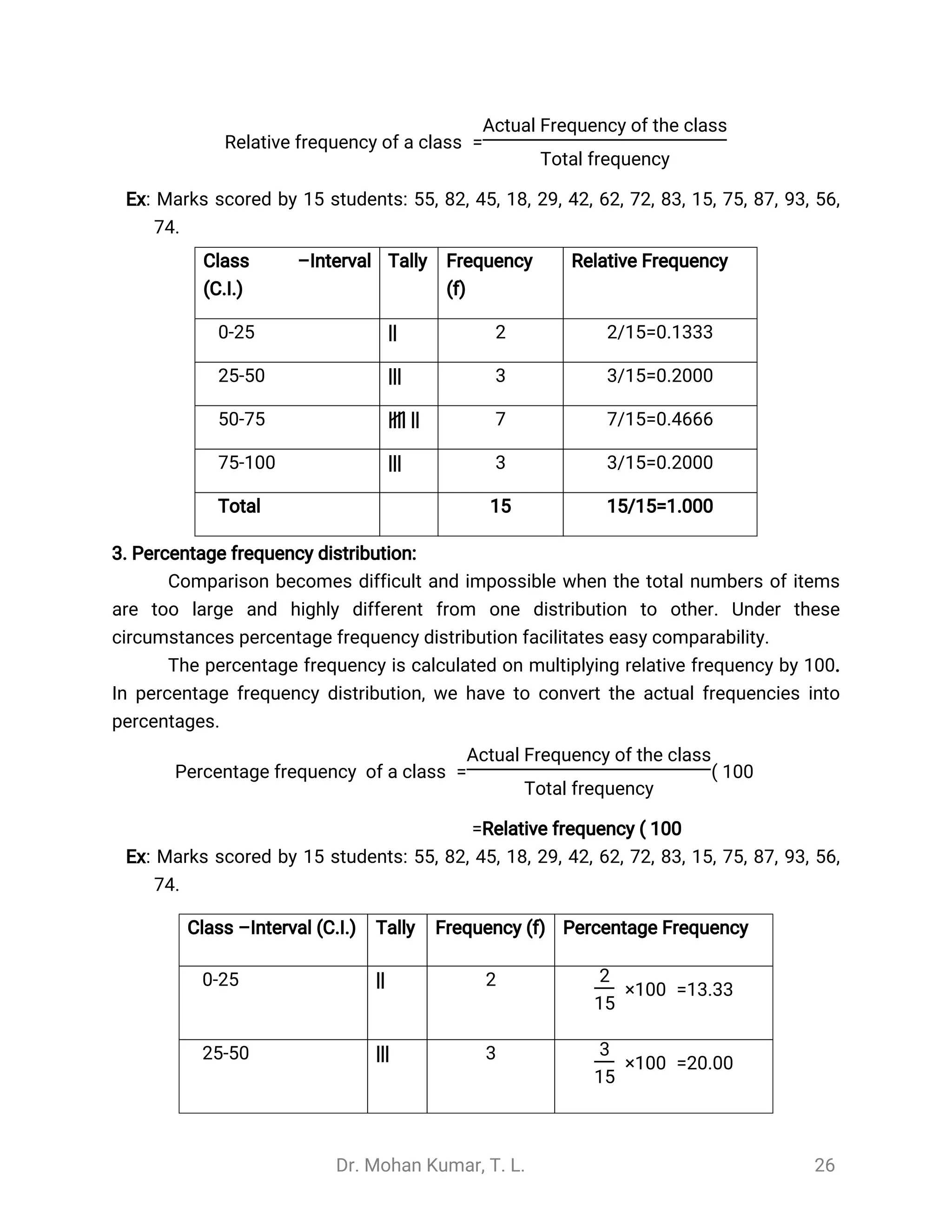
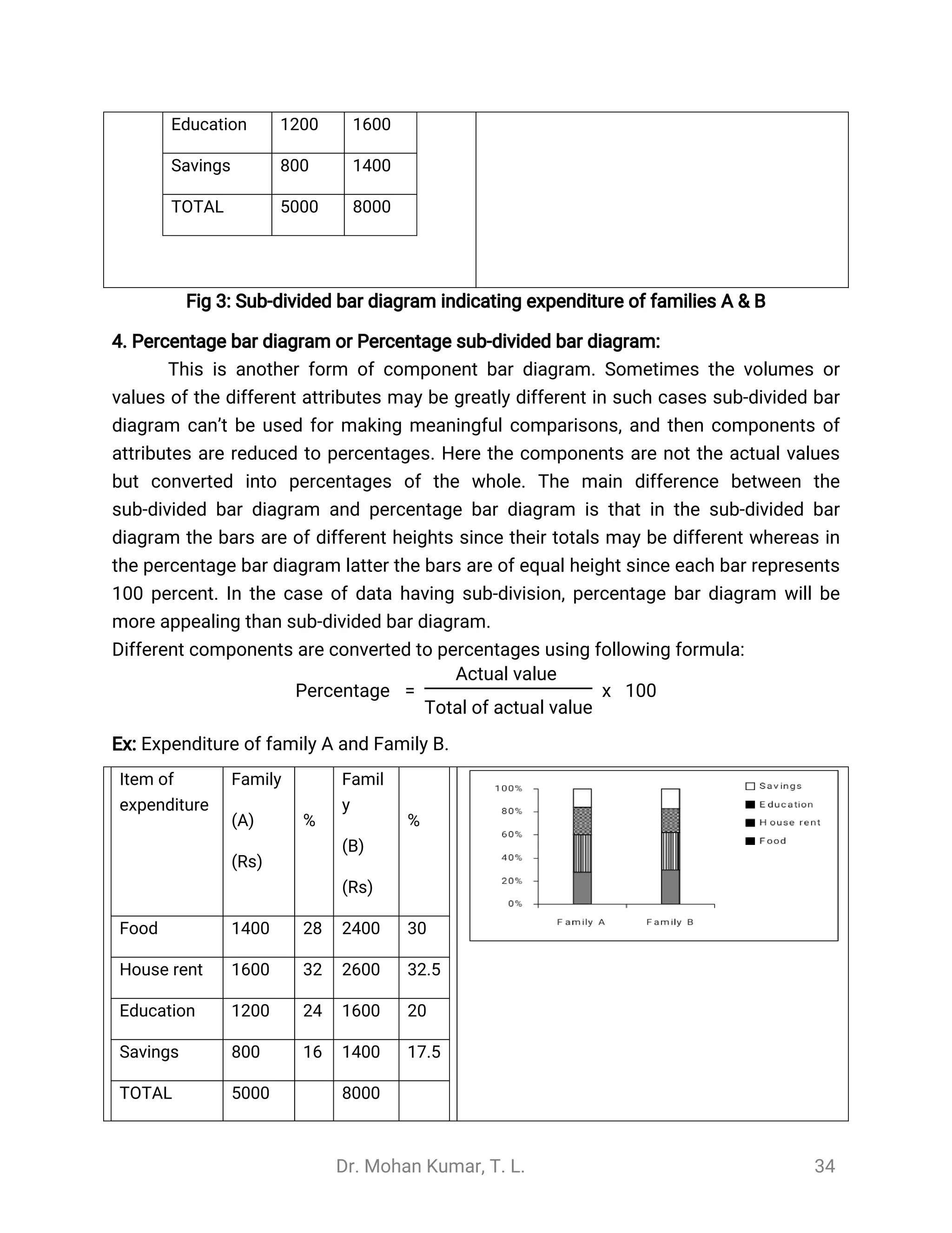
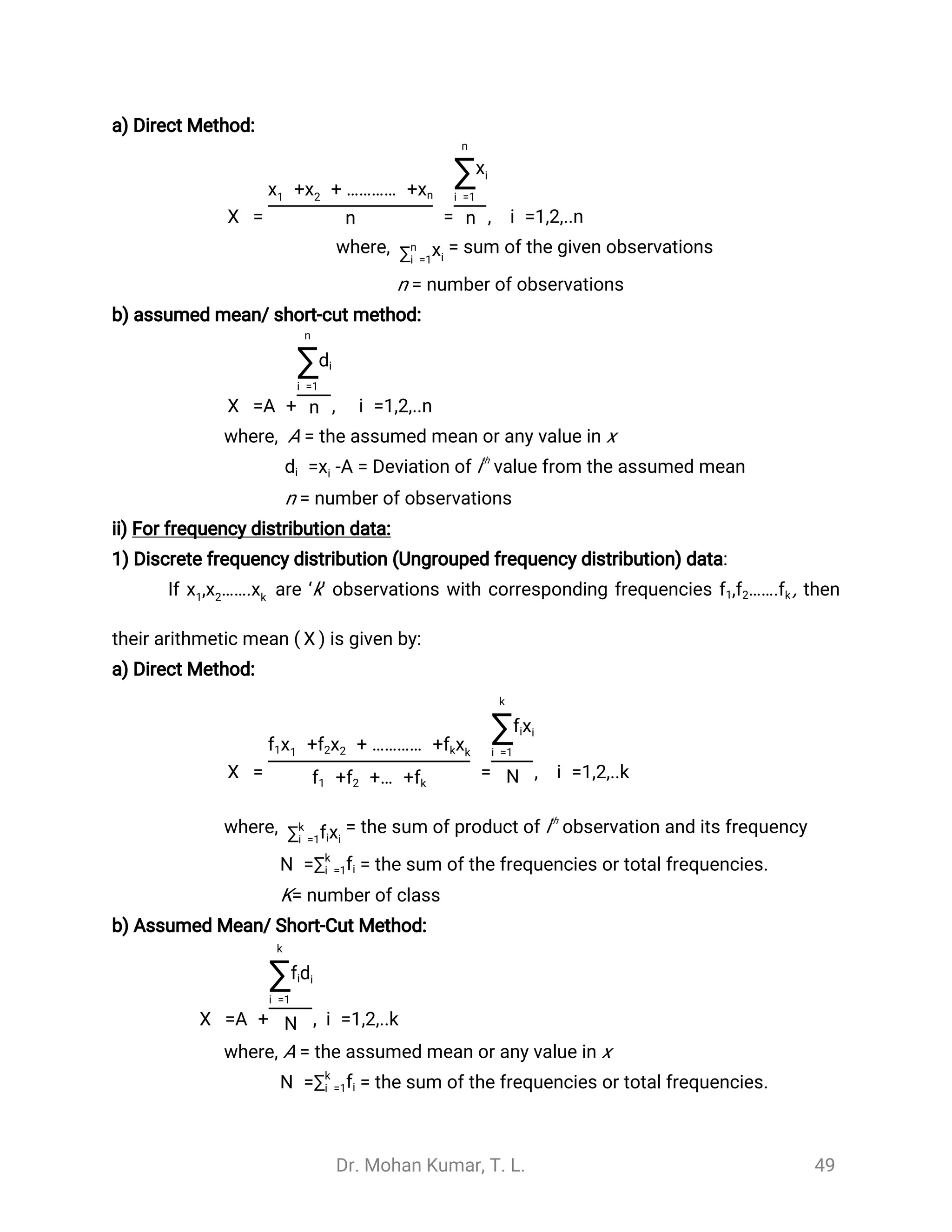
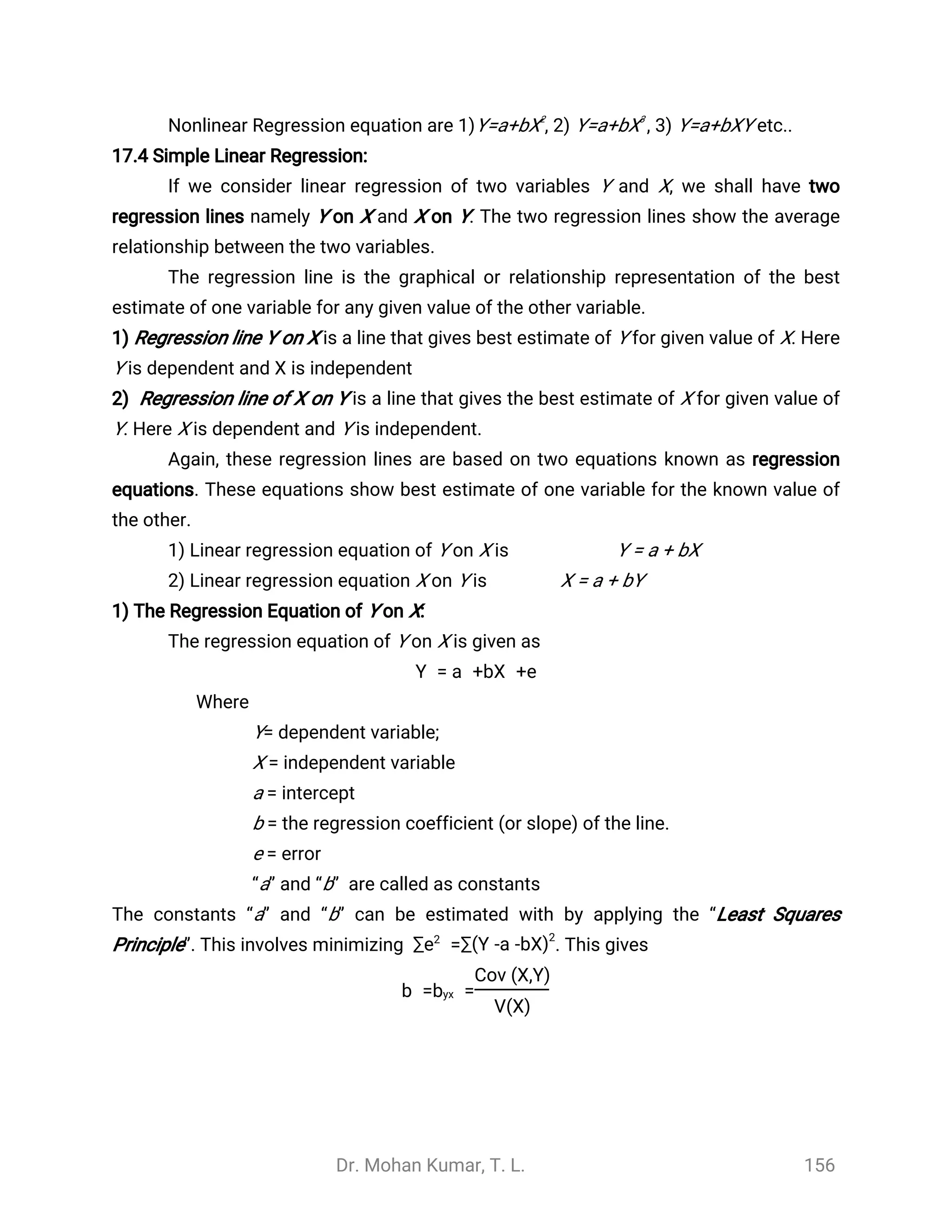
Step1: Find cumulative frequencies (CF).
Step2: Obtain total frequency (N) and Find . Where total frequencies
N
2
N =∑n
i =1fi
Step3: See in the cumulative frequency the value first greater than value. Then the(
N
2)
th
corresponding class interval is called the Median class.
Then apply the formula given below.
Median =Md = L +
[ ( c
-c.f.
N
2
f ]
Where, L = lower limit of the median class.
N = Total frequency
f = frequency of the median class
c.f. = cumulative frequency class preceding the median class
C = width of class interval.
Graphic method for Location of median:
Median can be located with the help of the cumulative frequency curve or ‘ogive’ .
The procedure for locating median in a grouped data is as follows:
Step1: The class boundaries, where there are no gaps between consecutive classes, i.e.
exclusive class are represented on the horizontal axis (x-axis).
Step2: The cumulative frequency corresponding to different classes is plotted on the
vertical axis (y-axis) against the upper limit of the class interval (or against the
variate value in the case of a discrete series.)
Step3: The curve obtained on joining the points by means of freehand drawing is called
the ‘ogive’ . The ogive so drawn may be either a (i) less than ogive or a (ii) more
than ogive.
Step4: The value of N/2 is marked on the y-axis, where N is the total frequency.
Step5: A horizontal straight line is drawn from the point N/2 on the y-axis parallel to
x-axis to meet the ogive.
Step6: A vertical straight line is drawn from the point of intersection perpendicular to the
horizontal axis.

Step7: The point of intersection of the perpendicular to the x-axis gives the value of the
median.
Fig 6.1: Graphic method for location of median
Remarks:
1. From the point of intersection of ‘ less than’ and ‘more than’ ogives, if a perpendicular
is drawn on the x-axis, the point so obtained on the horizontal axis gives the
value of the median.
Fig 6.2: Graphic method for location of median
Merits of Median:
1. It is easily understood and is easy to calculate.

3. It can be located merely by inspection.
4. It is not at all affected by extreme values.
5. It can be calculated for distributions with open-end classes.
6. Median is the only average to be used to study qualitative data where the items
are scored or ranked.
Demerits of Median:
1. In case of even number of observations median cannot be determined exactly.
We merely estimate it by taking the mean of two middle terms.
2. It is not based on all the observations.
3. It is not amenable to algebraic treatment.
4. As compared with mean, it is affected much by fluctuations of sampling.
5. If importance needs to be given for small or big item in the series, then median is
not suitable average.
Uses of Median
1. Median is the only average to be used while dealing with qualitative data which
cannot be measure quantitatively but can be arranged in ascending or
descending order.
Ex: To find the average honesty or average intelligence, average beauty etc...
among the group of people.
2. Used for the determining the typical value in problems concerning wages and
distribution of wealth.
3. Median is useful in distribution where open-end classes are given.
2) Mode:
The mode is the value in a distribution, which occur most frequently or
repeatedly.
It is an actual value, which has the highest concentration of items in and around
it or predominant in the series.
In case of discrete frequency distribution mode is the value of x corresponding to
maximum frequency.
Computation of mode:

Mode is the value of the variable (observation) which occurs maximum number
of times.
In case of discrete frequency distribution mode is the value of x variable
corresponding to maximum frequency.
If represents the mid-points of n class-interval, …….m1 m2 mk
with corresponding frequencies .- , - ,..., -- ,xx0 x1 1
x2 x2 x3 xn -1 xn , …….f1 f2 fk
Locate the highest frequency, and then the class-interval corresponding to
highest frequency is called the modal class.
Then apply the following formula, we can find mode:
Mode =Mo = L + ×C
-f1 f0
2 - -f1 f0 f2
Where, L = lower limit of the modal class.
C = Class interval of the modal class
= frequency of the class preceding the modal classf0
= frequency of the modal classf1
= frequency of the class succeeding the modal classf2
Graphic method for location of mode:
Steps:
1. Draw a histogram of the given distribution.
2. Join the top right corner of the highest rectangle (modal class rectangle) by a straight
line to the top right corner of the preceding rectangle. Similarly the top left corner
of the highest rectangle is joined to the top left corner of the rectangle on the
right.
3. From the point of intersection of these two diagonal lines, draw a perpendicular to the
x -axis.
4. Read the value in x-axis gives the mode.

Fig 6.3: Graphic method for Location of mode
Merits of Mode:
1. It is easy to calculate and in some cases it can be located mere inspection
2. Mode is not at all affected by extreme values.
3. It can be calculated for open-end classes.
4. It is usually an actual value of an important part of the series.
5. Mode can be conveniently located even if the frequency distribution has class
intervals of unequal magnitude provided the modal class and the classes
preceding and succeeding it are of the same magnitude.
Demerits of mode:
1. Mode is ill defined. It is not always possible to find a clearly defined mode.
2. It is not based on all observations.
3. It is not capable of further mathematical treatment.
4. As compared with mean, mode is affected to a greater extent by fluctuations of
sampling.
5. It is unsuitable in cases where relative importance of items has to be considered.
Remarks: In some cases, we may come across distributions with two modes. Such
distributions are called bi-modal. If a distribution has more than two modes, it is said to
be multimodal.
Uses of Mode:
Mode is most commonly used in business forecasting such as manufacturing
units, garments industry etc... to find the ideal size. Ex: in business forecasting for
manufacturing of readymade garments for average size of track suits, average size of
dress, average size of shoes etc....
3) Quantiles (or) Partition Values:
Quantiles are the values of the variable which divide the total number of

observations into number of equal parts when it is arranged in order of magnitude.
Ex: Median, Quartiles, Deciles, Percentiles.
i) Median: Median is only one value, which divides the whole series into two equal parts.
ii) Quartiles: Quartiles are three in number and divide the whole series into four equal
parts. They are represented by Q1, Q2, Q3 respectively.
First quratile: =Q1
(n +1)
4
Second quratile: =2Q2
(n +1)
4
=3Third quratile: Q3
(n +1)
4
iii) Deciles: Deciles are nine in number and divide the whole series into ten equal parts.
They are represented by D1, D2 …D9.
First Decile: =D1
(n +1)
10
Second Decile: =2D2
(n +1)
10
:
:
=9Ninth Decile: D9
(n +1)
10
iv) Percentiles: Percentiles are 99 in number and divide the whole series into 100 equal
parts. They are represented by P1, P2…P99.
First Percentile: =P1
(n +1)
100

Second Percentile: =2P2
(n +1)
100
:
=99Ninty nine Percentile: P99
(n +1)
100
8.8 Commercial Averages:
These are the averages which are mainly calculated based on needs in business.
Ex: Moving Average, Composite Average, Progressive Average
i) Moving Average (M.A.):
It is a special type of A.M. calculated to obtain a trend in time-series. We can find
M.A. by discarding one figure and adding next figure in sequentially and then computing
A.M. of the values which have be taken by rotation.
If a, b, c, d, and e are values in series, then M.A. is given by
M.A = , ,
a +b +c
3
b +c +d
3
c +d +e
3
ii) Progressive Average (P.A.):
It is a cumulative average used occasionally during the early years of the life of
business. This is computed by taking the entire figure available in each succeeding
years.
If a, b, c, d, and e are values in series, then P.A. is given by
P.A = , , ,
a +b
2
a +b +c
3
a +b +c +d
4
a +b +c +d +e
5
iii) Composite Average:

It is the average of different series. It is said to be the grand average because it is
an A.M. computed by taking out on average of various.
C.A =
+ +… +
̅
X 1
̅
X 2
̅
X n
number of series (n)
Some Important relation and results:
1. Relation between A.M., G.M. & H.M.
A.M. ( G.M. ( H.M.
2. i.e. G.M of A.M & H.M. is equal to G.M of two values.G.M. = A.M. ×H.M.
3. A.M. of first “n” natural number 1,2,3,....n is ( n+1)/2
4. Weighted A.M of first “n” natural number 1,2,3,....n with corresponding weights
1,2,3,...n is ( 2n+1)/3
5. If a and b are any two numbers, then A.M. = ; G.M. = ; H.M. =
a +b
2
a ×b
2ab
a +b

Chapter 9: MEASURES OF DISPERSION
9.1 Introduction
Measures of central tendency viz. Mean, Median, Mode, etc..., indicate the central
position of a series. They indicate the general magnitude of the data but fail to reveal all
the peculiarities and characteristics of the series. For example,
Series A: 20, 20, 20 SX = 60, A. M=20
Series B: 5, 10, 45 SX = 60, A. M=20
Series C: 17, 19, 24 SX = 60, A. M=20
In all the above three series, the value of arithmetic mean is 20. On the basis of
this average, we can say that the series are alike. But the pattern in which the
observations are distributed is different in different series. In series A, all observations
are same and equal to A.M., in series B & C all observations are different but their A.M.
is same as that of series A. Hence, Measures of Central tendency fail to reveal the
degree of the spread out or the extent of the variability in individual items of the
distribution. This can be explained by certain other measures, known as ‘Measures of
Dispersion’ or ‘Variation or Deviation’. Simplest meaning that can be attached to the
word ‘dispersion’ is a lack of uniformity in the sizes or quantities of the items of a
group.
9.2 Definition:
“Dispersion is the extent to which the magnitudes or quantities of individual
items differ, the degree of diversity.”
The dispersion or spread of the data is the degree of the scatter or variation of
the variable about the central value.
9.3 Properties/Characteristics/Pre-requisite of a Good Measure of Dispersion
There are certain pre-requisites for a good measure of dispersion:
1. It should be simple to understand and easy to compute.
2. It should be rigidly defined.
3. It should be based on each individual item of the distribution.
4. It should be capable of further algebraic treatment.
5. It should have less sampling fluctuation.
6. It should not be unduly affected by the extreme items.
7. It should be help for further Statistical Analysis.

9.3 Significance of measures of dispersion:
1) Dispersion helps to measure the reliability of central tendency i.e. dispersion enables
us to know whether an average is really representative of the series.
2) To know the nature of variation and its causes in order to control the variation.
3) To make a comparative study of the variability of two or more series by computing
the relative dispersion
4) Measures of dispersion provide the basis for studying correlation, regression,
analysis of variance, testing of hypothesis, statistical quality control etc...
5) Measures of dispersion are complements of the measures of central tendency. Both
together provide better tool to compare different distributions.
9.4 Types of Dispersion: Two types
1) Absolute measure of dispersion
2) Relative measures of dispersion.
1) Absolute measure of dispersion:
Absolute measures of dispersion are expressed in the same units in which the
original data are expressed/measured. For example, if the yield of food grains is
measured in Quintals, the absolute dispersion will also gives variation value in Quintals.
The only difficulty is that if two or more series are expressed in different units, the
series cannot be compared on the basis of absolute dispersion.
2) Relative or Coefficient of dispersion:
‘Relative’ or ‘Coefficient of dispersion’ is the ratio or the percentage of measure
of absolute dispersion to an appropriate average. Relative measures of dispersion are
free from units of measurements of the observation. They are pure numbers. The basic
advantage of this measure is that two or more series can be compared with each other
despite the fact they are expressed in different units.
Theoretically, absolute measure of dispersion is better. But from a practical point
of view, relative or coefficient of dispersion is considered better as it is used to make
comparison between series.
Absolute measure of dispersion Relative or Coefficient of
dispersion
1. Range Coefficient of Range

2. Quartile Deviation (Q. D.) Coefficient of Quartile Deviation
3. Mean Deviation(M.D.)/Average Deviation Coefficient of Mean Deviation
4. Standard deviation (S.D.) Coefficient of Standard Deviation
5. Variance Coefficient of Variation
1) Range:
It is the simplest method of studying dispersion. Range is the difference between
the Largest (Highest) value and the Smallest (Lowest) value in the given series. While
computing range, we do not take into account frequencies of different groups.
Range (R) = L-S
Where, L=Largest value
S= smallest value
Coefficient of Range =
L -S
L +S
Computation of Range:
i) For raw data/Individual series/ ungrouped data:
Range (R) = L-S
Where, L=Largest value in the series
S= smallest value in the series
ii) Frequency distribution data:
Range (R) = L-S
Where, L=Largest value of x variable
S= smallest value of x variable
Range (R) = L-S
Where, L = Upper boundary of the highest class
S = Lower boundary of the lowest class.
Merits of Range:
1. Range is a simplest method of studying dispersion.
2. It is simple to understand and easy to calculate.

4. It is useful in frequency distribution where only two extreme observation are
considers, middle items are not given any importance.
5. In certain types of problems like quality control, weather forecasts, share price
analysis, etc..., range is most widely used.
6. It gives a picture of the data in that it includes the broad limits within which all the
items fall.
Demerits of Range:
1. It is affected greatly by sampling fluctuations. Its values are never stable and
vary from sample to sample.
2. It is very much affected by the extreme items.
3. It is based on only two extreme observations.
4. It cannot be calculated from open-end class intervals.
5. It is not suitable for mathematical treatment.
6. It is a very rarely used measure.
7. Range is very sensitive to size of the sample.
Uses of Range:
1. Range is used for constructing quality control charts.
2. In weather forecasts, it gives max & min level of temperature, rainfall etc...
3. It’s used in studying variation in money rates, share price analysis, exchange
rates & gold prices etc., range is most widely used.
2) Quartile Deviation (Q.D.):
Quartile Deviation is half of the difference between the first quartile (Q1) and third
quartile (Q3). i.e.
Q.D. =
(Q3 - Q1)
2
The range between first quartile (Q1) and third quartile (Q3) is called by Inter
quartile range (IQR) i.e. IQR = Q3 - Q1.
Half of IQR is known as Semi Inter Quartile Range. Hence, Q.D. is also known
Semi Inter Quartile Range.
Co -efficient of Q.D. =
Q3 - Q1
Q3 + Q1

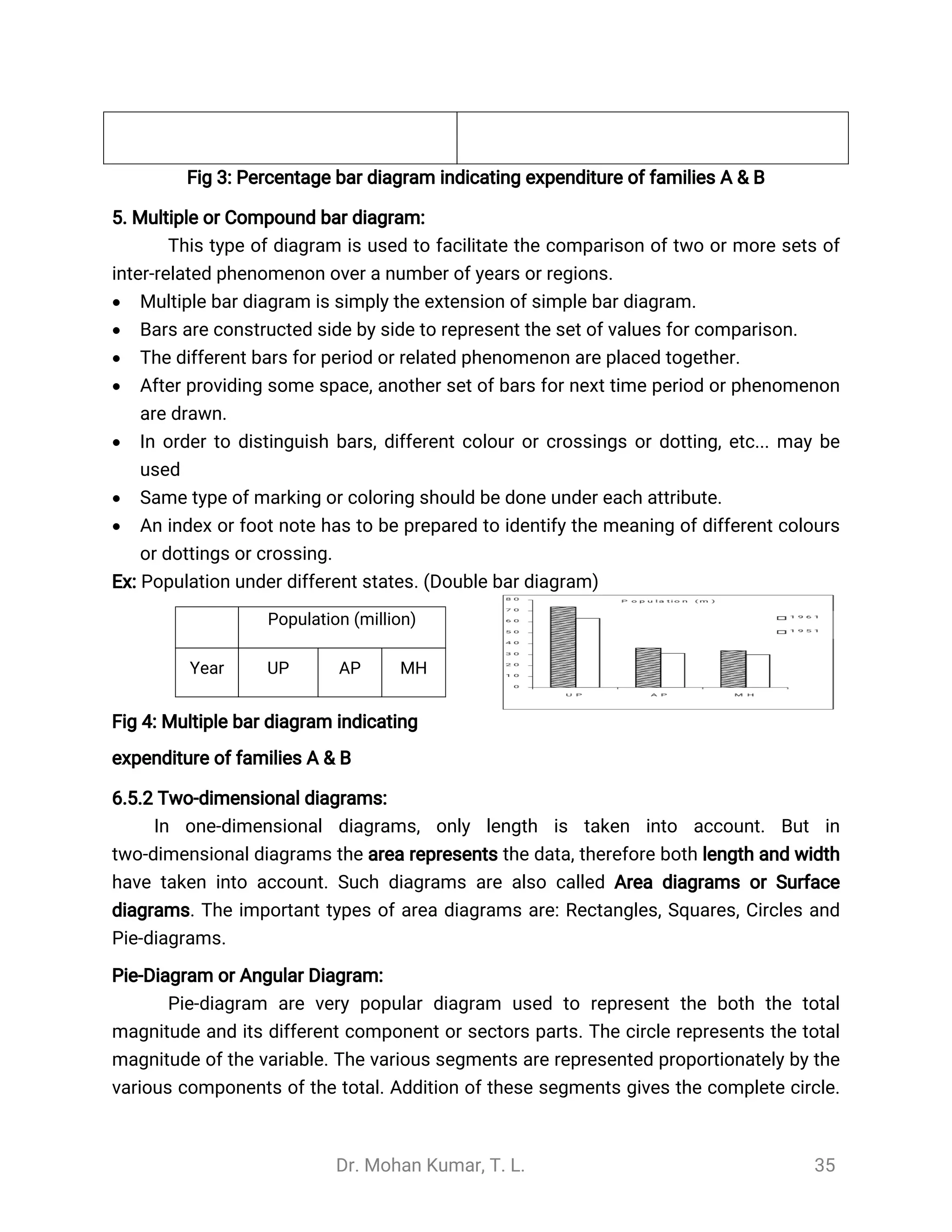
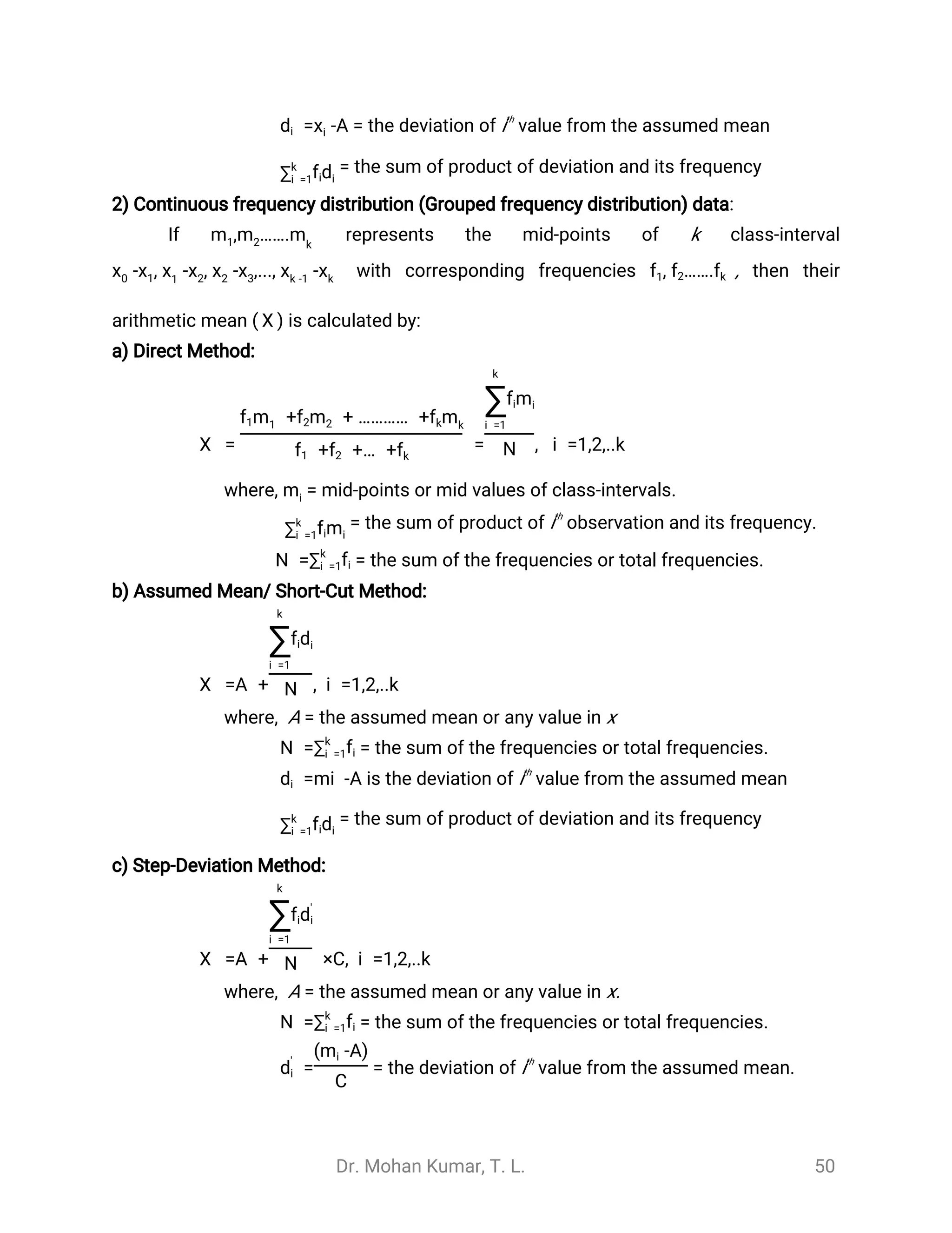
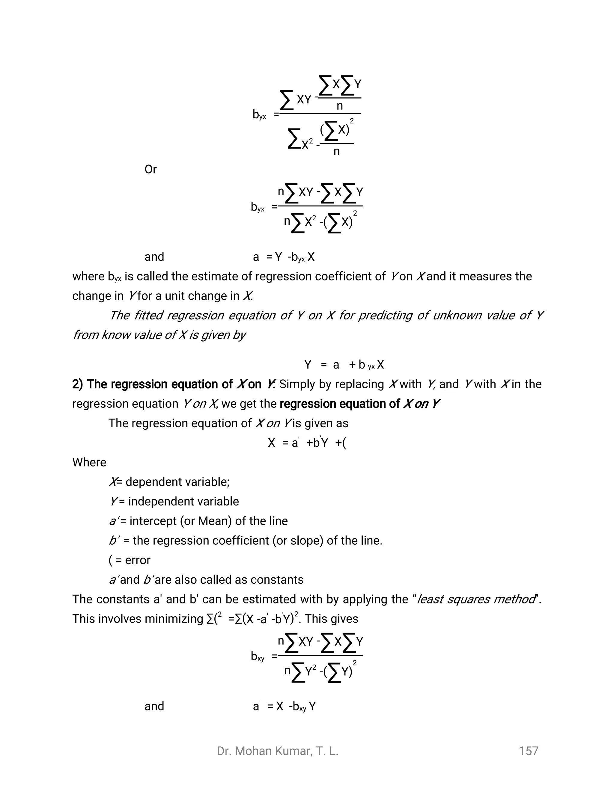
Computation of Q.D.:
Q.D. =
(Q3 - Q1)
2
Where
First quratile: =Q1 (
n +1
4 )
=3Third quratile: Q3 (
n +1
4 )
n= number of observations
Q.D. =
(Q3 - Q1)
2
Where
First quratile: =Q1 (
N +1
4 )
=3Third quratile: Q3 (
N +1
4 )
= Total frequencyN =∑k
i =1fi
Q.D. =
(Q3 - Q1)
2
Where
First quratile: = +Q1 L1
[ x
-
N
4
m1
f1
c1]
= +Third quratile: Q3 L3
[ x
3 -
N
4
m3
f3
c3]
Where, & = lower limit of the first & third quartile class.L1 L3
i =1fi

= frequency of the first & third quartile class&f1 f3
= cumulative frequency class preceding the first & third quartile class&m1 m3
= width of class intervals.&c1 c3
Merits of Q. D.:
1. It is simple to understand and easy to calculate.
3. It is not affected by the extreme values.
4. In the case of open-ended distribution, it is most suitable.
5. Since it is not influenced by the extreme values in a distribution, it is
particularly suitable in highly skewed distribution.
Demerits of Q. D.:
1. It is not based on all the items. It is based on two positional values Q1 and Q3 and
ignores the extreme 50% of the items.
2. It is not amenable to further mathematical treatment.
3. It is affected by sampling fluctuations.
4. Since it is a positional average, it is not considered as a measure of dispersion. It
merely shows a distance on scale and not a scatter around an average.
3) Mean Deviation (M.D.):
The range and quartile deviation are not based on all observations. They are
positional measures of dispersion. They do not show any scatter of the observations
from an average. The mean deviation is measure of dispersion based on all items in a
distribution.
Definition:
“Mean deviation is the arithmetic mean of the absolute deviations of a series
computed from any measure of central tendency; i.e., the mean, median or mode, all the
deviations are taken as positive”.
“Mean deviation is the average amount scatter of the items in a distribution from
either the mean or the median, ignoring the signs of the deviations”.
M.D =
∑| -A|xi
n
Where, M. D = Mean Deviation

A = any one Measures of Average i.e. Mean or Median or Mode
Co -efficient of M.D. =
M.D.
Mean or Median or Mode
Computation of M.D.:
M.D =
∑| -A|xi
n
= observationsxi
M.D =
∑ | -A|fi xi
N
= observationsxi
i =1fi
M.D =
∑ | -A|fi mi
N
= mid-point of class intervalsmi
i =1fi
Merits of M. D.:
1. It is simple to understand and easy to compute.
3. It is based on all items of the series.
4. It is not much affected by the fluctuations of sampling.

5. It is less affected by the extreme items.
6. It is flexible, because it can be calculated from any average.
Demerits of M. D.:
1. It is not a very accurate measure of dispersion.
2. It is not suitable for further mathematical calculation.
3. It is illogical and mathematically unsound to assume all negative signs as
positive signs.
4. Because the method is not mathematically sound, the results obtained by this
method are not reliable.
5. It is rarely used in sociological studies.
Uses of M.D.:
1) It is very useful while using small sample.
2) It is useful in computation of distributions of personal wealth in community or
nations, weather forecasting and business cycles.
Remarks:
1) Mean Deviation is minimum (least) when it is calculated from median than mean
or mode
2) Mean (15/2 M.D. includes about 99 % of observations.
3) Range covers 100 % of observations.
4) Standard Deviation (S.D.):
The concept of standard deviation, which was introduced by Karl Pearson in
1893, has a practical significance because it is free from all demerits, which exists in a
range, quartile deviation or mean deviation. It is the most important, stable & widely
used measure of dispersion. Standard deviation is also called Root-Mean Square
Deviation.
Definition:
It is defined as the positive square-root of the arithmetic mean of the square of
the deviations of the given observation from their arithmetic mean.
The standard deviation is denoted by the Greek letter ((sigma).
S.D. =(σ) ∑( - )xi
̅
X
2
n
Where, S.D. = Standard Deviation

= observationsxi
= Arithmetic Mean
̅
X
Co -efficient of S.D. =
S.D.
Mean ( )
̅
x
Computation of S.D.:
a) Deviations taken from Actual mean:
S.D. =
(σ) ∑( - )xi
̅
X
2
n
= observationsxi
= Arithmetic Mean
̅
X
b) Direct Method:
S.D. =(σ) -
∑x2
n (∑x
n
)
2
c) Short-cut method (Deviations are taken from assumed mean):
S.D. =(σ) -
∑d2
n (∑d
n
)
2
Where d-stands for the deviation from assumed mean = ( -A)xi
S.D. =
(σ) ∑fi( - )xi
̅
X
2
N

= observationsxi
= Arithmetic Mean
̅
X
= actual frequencyfi
i =1fi
b) Direct Method:
S.D. =(σ) -
∑fx2
N (∑fx
N
)
2
S.D. =(σ) -
∑fd2
N (∑fd
N
)
2
S.D. =(σ) ∑fi( - )mi
̅
x
2
N
= mid-points of class intervalsmi
= Arithmetic Mean
̅
X
= actual frequencyfi
i =1fi
b) Direct Method:
S.D. =(σ) -
∑fm2
N (∑fm
N
)
2
S.D. =(σ) -
∑fd2
N (∑fd
N
)
2
Where d-stands for the deviation from assumed mean = ( -A)mi

Mathematical properties of standard deviation (s)
7. S.D. of n natural numbers viz. 1,2,3...., n is calculated by
S.D. =(σ) ( -1)
1
12
n2
8. The sum of the squared deviations of the individual items from the arithmetic
mean is always minimum. i.e. ∑ = minimum( – )xi
̅
x
2
9. S.D. is independent on change of origin but not scale.
{ Change of Origin: If all values in the series are increased or decreased by a
constant, the standard deviation will remain the same.
Change of Scale: If all values in the series are multiplied or divided by a constant
than the standard deviation will be multiplied or divided by that constant.}
10.S.D. ( M.D. from Mean.
Merits of S. D.:
1. It is easy to understand.
3. Its value based on all the observations
4. It is possible for further algebraic treatment.
5. It is less affected by the fluctuations of sampling and hence stable.
6. As it is based on arithmetic mean, it has all the merits of arithmetic mean.
7. It is the most important, stable and widely used measure of dispersion.
8. It is the basis for calculating other several statistical measures like, co-efficient
of variance, coefficient of correlation, and coefficient of regression, standard
error etc...
Demerits of S. D.:
1. It is difficult to compute.
2. It assigns more weights to extreme items and less weights to items that are nearer
to mean because the values are squared up.
3. It can’t be determined for open-end class intervals.
4. As it is an absolute measure of variability, it cannot be used for the purpose of
comparison.
Uses of S. D.:
1. It is the most important, stable and widely used measure of dispersion.

2. It is very useful in knowing the variation of different series in making the test of
significance of various parameters.
3. It is used in computing area under standard normal curve.
4. It is used in calculating several statistical measures like, co-efficient of variance,
coefficient of correlation, and coefficient of regression, standard error etc...
5) Variance:
The term variance was given by R. A. Fisher for the first time in 1913 to describe
the square of the standard deviations. It is denoted by .σ
2
Variance is square of Standard Deviation. Similarly, Standard Deviation is the
square root of variance.
Definition:
The average of squared deviation of items in the series from their arithmetic
mean is called as Variance.
Variance ( ) =σ2
∑( - )xi
̅
x
2
n
Where, = Variance,σ2
= observationsxi
= Arithmetic Mean
̅
X
Computation of Variance:
=σ2
∑( - )xi
̅
X
2
n
b) Direct Method:
= -σ2
∑x2
n (∑x
n
)
2

= -σ2
∑d2
n (∑d
n
)
2
=σ2
∑fi( - )xi
̅
X
2
N
i =1fi
b) Direct Method:
= -σ2
∑fx2
N (∑fx
N
)
2
= -σ2
∑fd2
N (∑fd
N
)
2
=σ2
∑fi( - )mi
̅
X
2
N
= mid-points of class intervalsmi
b) Direct Method:
= -σ2
∑fm2
N (∑fm
N
)
2
= -σ2
∑fd2
N (∑fd
N
)
2

Where d-stands for the deviation from assumed mean = ( -A)mi
Remarks: 1) Variance is independent on change of origin but not scale.
{Change of Origin: If all values in the series are increased or decreased by a
constant, the Variance will remain the same.
Change of Scale: If all values in the series arc multiplied or divided by a constant
(k) than the Variance will be multiplied or divided by that square constant (k2
).}
Merits of Variance:
1. It is easy to understand and easy to calculate.
3. Its value based on all the observations.
4. It is possible for further algebraic treatment.
5. It is less affected by the fluctuations of sampling.
6. As it is based on arithmetic mean, it has all the merits of arithmetic mean.
7. Variance is most informative among the measures of dispersions.
Demerits of Variance:
1. The unit of expression of variance is not the same as that of the observations
because variance is indicated in squared deviation. Ex: if the observations are
measured in meter ( or in Kg), then variance will be in squares meters (or in kg
2
).
2. It can’t be determined for open-end class intervals.
3. It is affected by extreme values
4. As it is an absolute measure of variability, it cannot be used for the purpose of
comparison.
Coefficient of Variation (C.V.):
The Standard deviation is an absolute measure of dispersion. It is expressed in
terms of units in which the original figures are collected and stated. The standard
deviation of heights of plants cannot be compared with the standard deviation of weight
of the grains, as both are expressed in different units, i.e heights in centimeter and
weights in kilograms. Therefore the standard deviation must be converted into a relative
measure of dispersion for the purpose of comparison. The relative measure is known
as the coefficient of variation.
The coefficient of variation is obtained by dividing the standard deviation by the
mean and expressed in percentage.

Symbolically,
Coefficient of Variation = ×100(C.V.)
S.D
Mean
Coefficient of Variation = ×100(C.V.)
σ
̅
X
Remarks:
1. Generally, coefficient of variation is used to compare two or more series. If
coefficient of variation (C.V.) is more for series-I as compared to the series-II,
indicates that the population (or sample) of series-I is more variable, less stable,
less uniform, less consistent and less homogeneous. If the C.V. is less for
series-I as compared to the series-II, indicates that the population (or sample) of
series-I is less variable, more stable, or more uniform, more consistent and more
homogeneous.
2. A remark number 1 is applies for all the measures of dispersions.
3. All relative measure of dispersions are dependent on change of origin but
independent on change of scale.
4. Relationship between Q.D., M.D. & S.D. is
i) Q.D. = S.D.
2
3
M.D. = S.D.
4
5
6 Q. D.=5 M.D.=4 S.D.(
ii) S.D. > M.D.>Q.D.

Chapter 10: MEASURES OF SKEWNESS AND KURTOSIS
10.1 Introduction:
Various measures of central tendency & dispersions were discussed to reveal
clearly the silent features of frequency distributions. It is possible that two or more
frequency distributions may have the same central tendency (mean) & dispersions
(standard deviation) but may differ widely in their nature, composition & shapes or
overall appearance as can be seen from the following example:
In both these distributions the value of mean and standard deviation is the same
(Mean = 15, σ =5). But it does not imply that the distributions are alike in nature. The
distribution on the left-hand side is a symmetrical one whereas the distribution on the
right-hand side is asymmetrical or skewed. In these ways, measures of central
tendency & dispersions are inadequate to depict all the characteristics of distribution.
Measures of Skewness gives an idea about the shape of the curve & help us to
determine the nature & extent of concentration of the observations towards the higher
or lower values of the distributions.
10.2 Definition:
"Skewness refers to asymmetry or lack of symmetry in the shape of a frequency
distribution curve"
"When a series is not symmetrical it is said to be asymmetrical or skewed."
10.3. Symmetrical Distribution.
An ideal symmetrical distribution is unimodal, bell shaped curve. The values of
mean, median and mode coincide. Spread of the frequencies on both sides from the
centre point of the curve is same. Then the distribution is symmetrical distribution.

Symmetrical (Normal )distribution curve.
10.3 Asymmetrical Distribution:
A distribution, which is not symmetrical, is called a skewed distribution. The
values of mean, median and mode not coincide. The values of mean and mode are
pulled away and the value of median will be at the centre. Then this type of distribution
is called as Asymmetrical distribution or skewed distribution. Asymmetrical distribution
could either be positively skewed or negatively skewed.
10.4 Tests of Skewness:
There are certain tests to know skewness does exist in a frequency distribution.
1. In a skewed distribution, values of mean, median and mode would not coincide.
2. Quartiles will not be equidistant from median.
3. When asymmetrical distribution is drawn on the graph paper, it will not give a bell
shaped curve.
4. Sum of the positive deviations from the median is not equal to sum of negative
deviations.
10.5 Types of Skewness:
1) Positively Skewed distribution:
2) Negatively Skewed distribution
3) No Skewness/ Zero Skewness
1) Positively (right) skewed distribution:
The curve is skewed to right side, hence it is positively or right skewed
distribution. In a positively skewed distribution, the value of the mean is maximum and

that of the mode is least, the median lies in between the two. The frequencies are
spread out over a greater range of values on the right hand side than they are on the left
hand side.
2) Negatively skewed distribution:
The curve is skewed to left side, hence it is negatively or left skewed distribution.
In a negatively skewed distribution, the value of the mode is maximum and that of the
mean is least. The median lies in between the two. The frequencies are spread out over
a greater range of values on the left hand side than they are on the right hand side.
3) No Skewness/ Zero Skewness:
The curve is not skewed either to left side or right side, hence it is no/ zero
skewed distribution. In no skewness, the values of mean, median and mode are equal.
The frequencies are spread equally to right hand side and left hand side from center
value.
Remarks:
1. When the values of mean, median and mode are equal, there is no skewness.
2. When mean > median > mode, skewness will be positive.
3. When mean < median < mode, skewness will be negative.
10.6 Measures of Skewness:
Skewness can be studied graphically and mathematically. When we study
skewness graphically, we can find out whether skewness is positive or negative or zero.
This can be found with the help of above diagrams.
Mathematically skewness can be studied as:
(a) Absolute Skewness
(b) Relative or coefficient of skewness
When the skewness is presented in absolute term i.e, in original units of variables
measured, then it is absolute skewness. If the value of skewness is obtained in ratios or
percentages, it is called relative or coefficient of skewness.

If two or more series are expressed in different units, the series cannot be
compared on the basis of absolute skewness, when it is presented in relative,
comparison become easy.
Mathematical measures of skewness can be calculated by:
(1) Karl-Pearson’s Method
(2) Bowley’s Method
(3) Kelly ‘s Method
(4) Skewness based on moments
(1) Karl-Pearson’s Method:
According to Karl – Pearson, it involves mean, mode and standard deviation.
Absolute measures of skewness =Mean -Mode
Karl -Pearson’s Coefficient Skewness = =(Skp)
Mean – Mode
S.D.
-Mode
̅
X
σ
In case of mode is ill – defined, the coefficient can be determined by the formula:
Karl – Pearson’ s Co efficient Skewness = =(Skp)
3(Mean – Median)
S.D.
3( – Md)
̅
X
σ
Remarks:
1. For moderately skewed distribution, empirical relationship between mean,
median and mode is Mode = 3Median -2 Mean
( Mean - Mode = 3(Mean – Median)
2. Karl-Pearson’s coefficient of skewness ranges from -1 to +1. i.e. ≤1-1 ≤Skp
3. , Zero skewed=0, if =Md =MoSkp
̅
X
4. = +1, Positively skewedSkp
5. = -1, Negatively skewedSkp
(2) Bowley’s Method:
In Karl – Pearson’s method of measuring skewness requires the whole series to
calculation. Prof. Bowley has suggested a formula based on relative position of
quartiles. In a symmetrical distribution, the quartiles are equidistant from the value of
the median. Bowley’s method of skewness is based on the values of median, lower and

upper quartiles.
Absolute measures of skewness = + -2 MedianQ3 Q1
Bowley's Coefficient Skewness =(SkB)
+ -2 MedianQ3 Q1
-Q3 Q1
Where and are upper and lower quartiles.Q3 Q3
Remarks:
1. Bowley’s coefficient of skewness ranges from -1 to +1. i.e. ≤1-1 ≤SkB
2. Zero skewed=0,SkB
3. = +1, Positively skewedSkB
4. = -1, Negatively skewedSkB
5. Bowley’s coefficient of skewness also called as Quartile co-efficient of skewness.
It can be used in open-end class interval and when mode is ill defined.
6. One of main limitation in Bowley’s coefficient of skewness is that, it includes only
two extreme quartiles and is based on 50% of observation. It not covers all the
observations.
(3) Kelly’s method:
Kelly developed another measure of skewness, which is based on percentiles or
deciles.
Absolute measures of skewness =
+ -2P90 P10 P50
2
Kelly's Coefficient Skewness =(Skk)
+ -2P90 P10 P50
-P90 P10
Where are respectively tenth, fiftieth and ninetieth percentiles., & PP10 P50 90
Or
Absolute measures of skewness =
+ -2D9 D1 D5
2
Kelly's Coefficient Skewness =(Skk)
+ -2D9 D1 D5
-D9 D1
Where are respectively first, fifth and ninth deciles., & PD1 D5 9
(4) Skewness based on moments:
The measure of skewness based on moments is denoted by or and is givenβ1 γ1
by:

= or =β1
μ2
3
μ3
2
γ1
β1
10.7 Moments:
Moments refers to the average of the deviations from mean or origin raised to a
certain power. The arithmetic mean of various powers of these deviations in any
distribution is called the moments of the distribution about mean. Moments about
mean are generally used in statistics. The moments about the actual arithmetic mean
are denoted by μr. The first four moments about mean or central moments are as
follows:
moment = , r =1,2,3…krth
μr
∑( - )xi
̅
X
r
n
moment = =Zero (0)1st
μ1
∑( - )xi
̅
x
n
moment = =Variance2nd
μ2
∑( - )xi
̅
x
2
n
moment = =Skewness3rd
μ3
∑( - )xi
̅
x
3
n
moment = =kurtosis4th
μ4
∑( - )xi
̅
x
4
n
10.8 Kurtosis or Convexity of the frequency curve:
Kurtosis is another measure of the shape of a frequency curve. It is a Greek word,
which means ‘Bulginess’. While skewness signifies the extent of asymmetry, kurtosis
measures the degree of peakedness of a frequency distribution. Measures of kurtosis
denote the shape of top of a frequency curve.
Definition:
“Kurtosis’ is used to describe the degree of peakedness/flatness of a unimodal
frequency curve or frequency distribution”.
“Kurtosis is another measure, which refers to extent to which a unimodal
frequency curve is peaked/ flatted than normal curve”.

10.9 Types of Kurtosis:
Karl Pearson classified curves into three types on the basis of the shape of their
peaks.
1. Leptokurtic: If a curve is relatively narrower and peaked at the top than the normal
curve, it is designated as Leptokurtic.
2. Mesokurtic: Mesokurtic curve is neither too much flattened nor too much peaked. In
fact, this is the symmetrical (normal) frequency curve and bell shaped.
3. Platykurtic: If the frequency curve is more flat than normal curve, it is designated as
platykurtic.
These three types of curves are shown in figure below:
10.10 Measure of Kurtosis:
The measures of kurtosis for a frequency distribution based moments is denoted
by (2 or and is given byγ2
= or = -3β2
μ4
μ2
2
γ2
β2
1. If >3, the distribution is said to be more peaked and the curve is Leptokurtic.β2
2. If =3, the distribution is said to be normal and the curve is Mesokurtic.β2
3. If < 3, the distribution is said to be flat topped and the curve is Platykurtic.β2
Or
1. , the curve is Leptokurtic>0; +veγ2
2. the curve is Mesokurtic=0,γ2

3. , the curve is Platykurtic<0; -veγ2

Chapter 11: PROBABILITY
11.1 Introduction:
There are some events that occur in a certain or definite way for example
“direction in which the sunrises & sun set or person born in this earth will definitely die
s”. On the other hand, we come across number of events whose occurrence can’t be
predicted with certainty in advance, for example “whether it will rainy today”, “chance of
winning India in world cup final” “whether head appear in first toss of a coin”, “Seed
germination - either germinates or does not germinates”. etc... In these events, generally
people express their uncertainty (doubtful) expectation/estimation in the form of
chance or likelihood without knowing its true meaning. In statistical studies, we
generally draw conclusion about population parameter on the basis sample drawn from
the population, such inferences are also not certain. In all such cases we are not certain
about the result of experiments or have some doubts. So probability is related with
measures of doubt/uncertainty associated with prediction of results of those
experiments in advance. ‘Probably’, ‘likely’, ‘possibly’, ‘chance’, ‘may be’ etc... is some of
the most commonly used terms in our day-to-day conversation. All these terms more or
less convey the same sense.
“A probability is a quantitative measure of uncertainty - a number that conveys
the strength of our belief in the occurrence of an uncertain event”.
“Probability is the science of decision making with calculated risks in the face of
uncertainty”.
11.2 Introduction Elements to Set Theory:
Set: A collection or arrangement of well defined objects is called a set. Thos objects
which belong to the set are usually called as elements. Set are denoted by capital letter
A, B, C.... & its elements are denoted by small letters a,b,c... Generally set are represent
by curly bracket { }.
11.3 Form of Set:
1) Finite Set: Set contains finite (i.e. countable) number of elements are called finite
sets.
Ex: A: {a, e, i, o, u} -------> set of vowels
2) Infinite set: A set contains infinite (i.e. uncountable) number of elements is called
infinite set.
Ex: a) Number of stars in the sky,

b) Number of sand particle on beach,
d) Number of fish in oceans
3) Null Set or Empty set: A set which contains no elements at all is called as null or
empty set. It is denoted by (.
Ex: Set of natural number between 10 & 11, getting zero dots when we throw a die.
Remarks:
1) A set which is not a null set, which has at least one element, is called as
non-empty set.
2) {0} is not a null set, since it is containing zero as its one element.
3) {(} is not a null set, since it is contains null set as its element.
4) Sub set: If each elements of a set A is also an element of other set B, then set A is
called the Sub set of B. i.e A( B or B(A.Also we can say A is contained in B. where B
is super set of A.
Remarks:
1) Every set is subset of itself i.e. A( A
2) Null set is a sub set of every set i.e. ( ( A, (( B, (( C...
5) Equal Set: If A is sub set of B ( i.e. A( B) and B is sub set of A (i.e. B( A), then A& B are
said to be equal i.e. A=B.
6) Equivalent Set: Two sets are said to be equivalent set, if they contain the same
number of elements i.e if n(A)=n(B).
7) Universal Set: Any set which contains many set is known as universal set. It is always
denoted by S or U.
11.4 Operation on Set:
1) Union of Sets: Union of two sets A & B is the set consisting of elements which belong
to either A or B or both (At least one of them should occur/happen).
Symbolically: A(B={x: x(A or x(B}
Ex: U= {a, b, c, d, e, f}, A= {a, b, c, d}, B={b, d, e, f}
Then A or B =A(B = {a, b, c, d, e, f}

2) Intersection of sets: Intersection of two sets A & B is the set consisting of elements,
which are common in both A & B sets.
Symbolically: A and B = A(B ={x: x(A and x(B}
Ex: if U= {a, b, c, d, e, f}, A= {a, b, c, d}, B={b, d, e, f}
Then A and B =A(B = {b, d}
3) Disjoint or Mutually exclusive sets: If sets A & B are said to be disjoint set if
intersection of them is the null set i.e. A(B=(
4) Complement of sets: The complement of set A is the set of elements which do not
belongs to set A, but belongs to universal set S. it is denoted by or .A'
̅
A
Symbolically: ={x: x(A and x(S}
̅
A
Ex: if U = {a, b, c, d, e, f}, A= {a, b, c, d}, B={b, d, e, f}
Then = {e, f }
̅
A
5) Difference of two sets: The difference of two sets A & B, which is denoted by A-B is
the set of elements which belongs to A but not belongs to B.
Symbolically: A - B = {x: x(A and x(B}
Ex: if if U = {a, b, c, d, e, f}, A= {a, b, c, d}, B={b, d, e, f}
Then A-B = {a, c }, B-A ={e,f}
11.5 Some Basic Concepts of Probability:

1) Experiment:
Any operation on certain objects or group of objects that gives different well
defined results is called an experiment. Different possible results are known as its
outcomes.
Ex: Drawing a card out of a deck of 52 cards, or reading the temperature, or pest
is exposed to pesticide, or seed is sown for germination or the launching of a new
product in the market, constitute an experiment in the probability theory.
2) Random experiment:
Under identical conditions, an experiment which does not gives unique results
but have any of the possible results which can’t be predict in advance is called random
experiment.
An experiment having more than one possible outcome that cannot be predicted
in advance.
Ex: Tossing of coins, throwing of dice are some examples of random
experiments.
3) Trail: Each performance in a random experiment is called a trial.
Ex: Tossing of coin one or more times, a seed or set of seed are sown for germination
4) Outcomes:
The results of a random experiment/trail are called its outcomes.
Ex: 1) When two coins are tossed the possible outcomes are HH, HT, TH, TT.
2) Seed germination – either germinates or does not germinates are
outcomes.
5) Sample space (S)
A set of all possible outcomes of a random experiment is called sample space. It
is denoted by S. Each possible outcome (or) element in a sample space is called
sample point.
Ex: 1) Set of five seeds are sown: none may germinate, 1, 2, 3 ,4 or all five may
germinate.
S= {0, 1, 2, 3, 4, 5}. The set of numbers is called a sample space. Number 0, 1, 2,
3, 4, & 5 are sample elements.
2) When a coin is tossed
The sample space is S = {H, T}. H and T are the sample points.
3) Throwing single die:

The sample space is S= {1,2,3,4,5,6}; number 1, 2,3,4,5,&6 are sample elements.
6) Event:
An outcome or group of outcomes of a random experiment is called an event.
Ex:1) In tossing two coin,
A: getting single head,
B: getting two tail
2) For the experiment of drawing a card.
A : The event that card drawn is king of club.
B : The event that card drawn is red.
C : The event that card drawn is ace.
In the above example A, B, & C are different events
11.6 Types of Events:
1) Equally likely events:
Two or more events are said to be equally likely if each one of them has an equal
chance of occurring.
Ex: In tossing of a coin, the event of getting a head and the event of getting a tail are
equally likely events.
2) Mutually exclusive events or incompatible events:
Two or more events are said to be mutually exclusive, when the occurrence of any
one event excludes the occurrence of all the other events. Mutually exclusive events
cannot occur simultaneously. If two events A and B are mutually exclusive events, then
A(B=(
Ex: 1) when a coin is tossed, either the head or the tail will come up. Therefore the
occurrence of the head completely excludes the occurrence of the tail. Thus
getting head or tail in tossing of a coin is a mutually exclusive event.
2) In observation of seed germination the seed may either germinate or it will not
germinate. Germination and non germination are mutually exclusive events.
3) Exhaustive events:
The total number of possible outcomes of a random experiment is called as
exhaustive events/cases.

Ex: 1) While throwing a die, the possible outcomes are {1, 2, 3, 4, 5, 6}, here the number
of exhaustive cases is 6.
2) When pesticide exposed to pest, pest may die or survives, here two exhaustive
cases ie one is die and another is survive.
3) In observation of seed germination the seed may either germinate or it will not
germinate, here two exhaustive cases ie germinate and not germinate.
4) Complementary events:
The event “A occurs” and the event “A does not occur” are called complementary
events to each other. The event ‘A does not occur’ is denoted by A' or or Ac
. The event
̅
A
and its complements are mutually exclusive.
Ex: In throwing a die, the event of getting odd numbers is { 1, 3, 5 } and getting even
numbers is {2, 4, 6}.These two events are mutually exclusive and complement to
each other.
5) Favourable Events:
The number of outcomes which entail the happening of particular event is the
number of cases favourable to that event.
Ex: When 5 seed are sown to know germination percentage, then events are
A: At least three seeds germinated.
Then favorable cases are 3, 4 & 5 seed germinated
B: Maximum two seeds germinated.
Then favorable cases are 0,1 & 2 seeds germinated.
6) Null Event (Impossible event):
An event which doesn’t contain any outcome of sample space is called Null
Event; it is denoted by ‘(’.
Ex: A: Happening of zero number when we thrown a die.
A = ( or A = { }
7) Simple or elementary event: An event which has only one outcome is called simple
event.
Ex: A: Happening of both heads when we toss two coin at a time
A= {HH}
8) Compound event: An event which has more than one outcome is called compound
event.

Ex: A: Happening of odd numbers when we thrown a die; A= {1, 3, 5}
9) Sure event or Certain Event: An event which contains all the outcomes which is equal
to sample space is called Sure Event.
Ex: A: Happening of number less than or more than 3, when we thrown a die.
A= {1, 2, 3, 4, 5, 6}
10) Independent Events:
If two or more events are said to be independent if the happening of an event is
not affected by the happening of one or more other events.
Ex: When two seeds are sown in a pot, one seed germinates. It would not affect the
germination or non germination of the second seed. One event does not affect the
other event.
11) Dependent Events:
If the happening of one event is affected by the happening of one or more events,
then the events are called dependent events.
Ex: If we draw a card from a pack of well shuffled cards, if the first card drawn is not
replaced then the second draw is dependent on the first draw.
11.7 Definition of Probability:
There are 3 approaches:
1) Mathematical (or) Classical (or) a-priori Probability
2) Statistical (or) Empirical Probability (or) a-posteriori Probability
3) Axiomatic approach to probability
1) Mathematical (or) Classical (or) A-Priori Probability (by James Bernoulli)
If a random experiment or trails results in ‘n’ exhaustive, mutually exclusive and
equally likely cases, out of which ‘m’ events are favourable to the happening of an event
‘A’, then the probability (p) of happening of ‘A’ is given by:
P =p = = =(A)
Number of cases favourable to the event A
Total number of exhaustive cases
n(A)
n(S)
m
n
Where, n(A)=m= number of favourable cases to an event A
n(S)= n= number of exhaustive cases
Remarks:
1) If m = 0 ⇒ P(A)=p = 0, then ‘A’ is called an impossible event.
2) If m = n ⇒ P(A) = 1, then ‘A’ is called sure (or) certain event.

3) P(φ) = 0 ( probability of null event is always zero
4) P(S) = 1 ( probability of sample space is always one
5) The probability is a non-negative real number and cannot exceed unity
i.e. 0 ( P(A) ( 1 (i.e. probability lies between 0 to 1)
6) The probability happening of the event A is P(A) and denoted by ‘p’.
The probability non-happening of the event A is , and denoted by ‘q’.P( )
̅
A
Then (total probabilityP +P =1(A) (̅
A )
( p+q=1
⇒ q = 1 – p
7) Mathematical probability is often called classical probability or a-priori probability
because if we keep using the examples of tossing of fair coin, dice etc., we can
state the answer in advance (prior), without tossing of coins or without rolling the
dice etc.,
Drawbacks of Mathematical probability:
The above definition of probability is widely used, but it cannot be applied under
the following situations:
(1) If it is not possible to enumerate all the possible outcomes for an experiment.
(2) If the sample points (outcomes) are not mutually independent.
(3) If the total number of outcomes is infinite.
(4) If each and every outcome is not equally likely.
2) Statistical (or) Empirical Probability (or) a-posteriori Probability or relative frequency
approach (by Von Mises)
If the probability of an event can be determined only after the actual happening of
the event, it is called Statistical probability.
If an experiment is repeated sufficiently (infinitely) large number of times under
homogeneous and identical condition, if ‘m’ events are favourable to the happening of
an event ‘A’ out of ‘n’ events, then its relative frequency is ‘m/n’. The statistical
probability of happening of ‘A’ is given by:
P =p =(A) lim
n→∞
m
n
Remarks: The Statistical probability calculated by conducting an actual experiment is
also called a posteriori probability or empirical probability.

Drawbacks:
1) It fails to determine the probability in the cases when the experimental conditions
don’t remains identically homogeneous.
2) The relative frequency (m/n) may not attain a unique value because actual limiting
value may not really exist.
3) The concept of infinitely large number of observation is theoretical and
impracticable.
3) Axiomatic approach to probability: (by A.N. Kolmogorov in 1933)
The modern approach to probability is purely axiomatic and it is based on the set
theory.
Axioms of probability:
Let ‘S’ be a sample space and ‘A’ be an event in ‘S’ and P(A) is the probability
satisfying the following axioms:
(1) The probability of any event ranges from zero to one. i.e 0 ( P(A) ( 1
(2) The probability of the entire space is 1. i.e P(S) = 1
(3) If A1, A2,…An is a sequence of n mutually exclusive events in S, then
P =P +P +… +P( )( ∪ ∪… ∪A1 A2 An) (A1) (A2) An
Properties of Probability:
1) 0 ( P(A) ( 1 i.e. probability lies between 0 to 1
2) P(φ) = 0 ( probability of null event is always zero
3) P(S) = 1 ( probability of sample space is always one
4) The probability happening of the event A is P(A) and denoted by ‘p’.
The probability non-happening of the event A is , and denoted by ‘q’.P( )
̅
A
Then (total probabilityP +P =1(A) (̅
A )
p+q=1 ⇒ q = 1 – p
5) If m = 0 ⇒ P(A)=p = 0, then ‘A’ is called an impossible event.
6) If m = n ⇒ P(A) = 1, then ‘A’ is called sure (or) certain event.
11.8. Permutation and Combinations:
1) Permutation:
Permutation means arrangement of things in different ways. The number of way

of arranging ‘r’ objects selected from ‘n’ objects in order is given by
=nPr
n!
!(n -r)
Where ! is factorial,
n!= n*(n-1)*(n-2)*....3*2*1
Remarks: (a) 0!=1, (b)
n
pn=n!, (c)
n
p0=1, (d)
n
p1=n
2) Combination:
A combination is a selection of objects from group of objects without
considering the order of arrangements. The number of combination is the number of
way of selecting ‘r’ objects from ‘n’ objects when order of arrangement is not important
is given by:
=nCr
n!
!r!(n -r)
Remarks: (a)
n
Cn=1, (b)
n
C0=1, (c)
n
C1=n, (d) , (e)
n
pr =r! * n
Cr=nCr
nPr
r!
11.9 Theorems of Probability:
There are two important theorems of probability namely,
1. The addition theorem on probability
2. The multiplication theorem on probability.
1) The addition theorem on probability: Here we have two cases
Case I: when events are not mutually exclusive:
If A and B are any two events which are not mutually exclusive, then probability of
occurrence of at least one of them (either A or B or both) is given by:
P =P =P +P -P(A (B)(A or B) (A ∪B) (A) (B)
For three events A, B & C: P(A or B or C)
P =P +P +P -P -P -P +P(A (B(C)(A ∪B ∪C) (A) (B) (C) (A (B) (A (C) (B (C)
Case II: when events are mutually exclusive:
If A and B are any two events which are mutually exclusive, then probability of
occurrence of at least one of them (either A or B or both) is the sum of the individual
probability of A & B given by:
P =P =P +P(A or B) (A ∪B) (A) (B)
For three events A, B & C:
P =P =P +P +P(A or Bor C) (A ∪B ∪C) (A) (B) (C)

Note: In mutually exclusive cases (A (B) =(, ( P =((A (B)
2) The multiplication theorem on probability: Here also two cases
Case I: when events are independent:
If A and B are any two events said to independent events, then probability of
occurrence of both them is equal to the product of their individual probabilities is given
by:
P =P =P .P(A and B) (A(B) (A) (B)
P P =P .P .P(A and B and C) (A(B(C) (A) (B) (C)
Case II: when events are Dependent:
If A and B are any two dependent events, then the probability that both A and B
will occur is
P =P =P .P ; P >0(A and B) (A(B) (A) (B/A) (A)
P =P =P .P ; P >0(A and B) (A(B) (B) (A/B) (B)
P (A∩B∩C) = P (A). P (B/A). P (C/A∩B)
11.10 Conditional Probability:
If two events ‘A’ and ‘B’ are said to be dependent with P(A) >0, then the
probability that an event ‘B’ occurs subject to the condition that ‘A’ has already occurred
is known as the conditional probability of the event ‘B’ on the assumption that the event
‘A’ has already occurred. It is denoted by the symbol P(B/A) or P(B|A) and read as the
probability of B given A.
If two events A and B are dependent, then the conditional probability of B given A
is
P(B/A) = ; P(A) >0
P(A(B)
P(A)
Similarly, if two events A and B are dependent, then the conditional probability of
A given B is denoted by P(A/B) or P(A|B) is
P(A/B) = ; P(B) >0
P(A(B)
P(B)

Chapter 12: Theoretical Probability Distributions
12.1. Introduction:
If an experiment is conducted under identical conditions, the observations may
vary from trail to trail. Hence, we have a set of outcomes (sample points) of a random
experiment. A rule that assigns a real number to each outcome (sample point) is called
random variable.
12.2. Random variable:
A variable whose value is a real number determined by the outcome of a random
experiment is called a random variable. Generally, a random variable is denoted by
capital letters like X, Y, Z….., where as the values of the random variable are denoted by
the corresponding small letters like x, y, z …….
Suppose that two coins are tossed so that the sample space is S = {HH, HT, TH,
TT}
Suppose X is the number of heads which can come up, with each sample point we can
associate a number for X as shown in the table below:
Sample
point
HH HT TH TT
X 2 1 1 0
Random variable may be discrete or continuous random variable
1) Discrete random variable:
If a random variable takes only finite or countable number of values, then it is
called discrete random variable. Ex: when 3 coins are tossed, the number of heads
obtained is the random variable X assumes the values 0,1,2,3 which form a countable
set.
2) Continuous random variable:
A random variable X which can take any value between certain intervals is called
a continuous random variable. Ex: the height of students in a particular class lies
between 4 feet to 6 feet.
12.3 Probability distributions:
If all the possible outcomes of random experiment associated with
corresponding probability is called probability distributions.
Following condition should hold:

(1) andP ≥0(X =xi)
(2) ∑P =1(X =xi)
In tossing two coins example, is the probability function given as,P(X =xi)
Sample
point
HH HT TH TT
X 2 1 1 0
P(X =xi) 1/
4
1/
4
1/
4
1/
4
1) Probability mass function (pmf) & discrete probability distribution:
If the random variable X is a discrete random variable, the probability function
is called probability mass function and its distribution is called discreteP(X =xi)
probability distribution. It satisfies the following conditions:
(i) andP ≥0(X =xi)
(ii) ∑P =1(X =xi)
Ex: for discrete probability distribution:
1) Bernoulli Distributions
2) Binomial Distributions
3) Poisson Distributions
2) Probability density function (pdf) & Continuous probability distribution:
If the random variable X is a continuous random variable, the probability function
is called probability density function and its distribution is called continuousf(X =xi)
probability distribution.
It satisfies the following conditions:
(i) andf ≥0(X =xi)
(ii) ∫f =1(X =xi)
Ex: for discrete probability distribution
1) Normal Distributions
2) Standard Normal Distributions

12.4. Probability mass function/Discrete probability distribution:
1) Bernoulli distributions: (Given by Jacob Bernoulli):
Bernoulli distributions is based on Bernoulli trails. A Bernoulli trial is a random
experiment in which there are only two possible/dichotomous outcomes consists of
success or failure. Ex: for Bernoulli’s trails are:
1) Toss of a coin (head or tail)
2) Throw of a die (even or odd number)
3) Performance of a student in an examination (pass or fail)
4) Germination of seed (germinate or not) etc...
Definition: A random variable x is said to follow Bernoulli distribution, if it takes only two
possible values 1 and 0 with respective probability of success ‘p’ and probability of
failure ‘q’ i.e., P(x=1) = p and P(x=0) = q, q = 1-p, then the Bernoulli probability mass
function is given by
P =(X =xi)
{
; x =0 & 1px
q1 -x
0 otherwise
Where x= Bernoulli variate, p=probability of success, and q=probability of failure

Constant/characteristics of Bernoulli distribution:
Parameter of model is p
1) Mean = E(X) = p
2) Variance = V(X)= pq
3) Standard Deviation = SD(X)= pq
2) Binomial distributions:
Binomial distribution is a discrete probability distribution which arises when
Bernoulli trails are performed repeatedly for a fixed number of times say ‘n’.
Definition: A random variable ‘x’ is said to follow binomial distribution if it assumes
nonnegative values and its probability mass function is given by
P =(X =xi)
{
; x =0, & 1,2,3…npnCx
x
qn -x
0 otherwise
The two independent constants ‘n’ and ‘p’ in the distribution are known as the
parameters of the distribution.
Condition/assumptions of Binomial distribution:
We get the Binomial distribution under the following experimental conditions.
1) The number of trials ‘n’ is finite.
2) The probability of success ‘p’ is constant for each trial.
3) The trials are independent of each other.
4) Each trial must result in only two possible outcomes i.e. success or failure.
The problems relating to tossing of coins or throwing of dice or drawing cards
from a pack of cards with replacement lead to binomial probability distribution.
Constant of Binomial distribution:
Parameter of model are n & p
1) Mean = E(X) = np
2) Variance = V(X)= npq
Standard Deviation = SD(X) = npq
3) Coefficient of Skewness = q -p
npq
4) Coefficient Kurtosis =
1 -6pq
npq
5) Mode of the Binomial distribution is that value of the variable x, which occurs
Mean >Variance

with the largest probability. It may have either unimode or bimode.
Importance/Situation of Binomial Distribution:
1) In quality control, officer may want to know & classify items as defectives or
non-defective.
2) Number of seeds germinated or not when a set of seeds are sown
3) To know the plants diseases occurrence or not occurrence among plants.
4) Medical applications such as success or failure, cure or no-cure.
3) Poisson distribution:
The Poisson distribution, named after Simeon Denis Poisson (1781-1840). It
describes random events that occur rarely over a unit of time or space. Also, it is
expected in cases where the chance or probability of any individual events being
success is very less to describe the behaviour of rare events such as number of
accident on road, number of printing mistakes in a books etc...
It differs from the binomial distribution in the sense that we count the number of
success and number of failures, while in Poisson distribution, the average number of
success in given unit of time or space.
Poisson distribution is derived as limiting cases of Binomial distribution by
relaxing first two of 4 conditions of Binomial distribution, i.e.
1) Number of trail “n” is very large i.e. n((
2) Probability of success is very rare/small i.e p (0
So that the product np=( is non-negative and finite.
Definition:
If x is a Poisson variate with parameter ( =np, then the probability that exactly x
events will occur in a given time is given by Probability mass function as:
P =(X =xi)
{
; x =0, & 1,3…∞
e -λ
λ
x
x!
0 otherwise
Where ( is known as parameter of the distribution so that ( >0
X= Poisson variate....
e=2.7183
Constant of Poisson distribution:
Parameter of model is (

1) Mean = E(X) = (
2) Variance = V(X)= (
3) Standard Deviation = SD(X) = (
4) Coefficient of Skewness is = 1
(
5) Coefficient Kurtosis = 3 +
1
(
Some examples of Poisson variates are:
1. The number of blinds born in a town in a particular year.
2. Number of mistakes committed in a typed page.
3. The number of students scoring very high marks in all subjects
4. The number of plane accidents in a particular week.
5. Number of suicides reported in a particular day.
6. It is used in quality control statistics to count the number of defects of an item.
7. In biology, to count the number of bacteria.
8. In determining the number of deaths in a district in a given period, by rare
disease.
10. The number of plants infected with a particular disease in a plot of field.
11. Number of weeds in particular species in different plots of a field.
12.5. Probability density function/Continuous probability distribution:
1) Normal Distribution:
Normal probability distribution or simply normal distribution is most important
continuous distribution because it plays a vital role in the theoretical and applied
statistics. The normal distribution was first discovered by De Moivre, English
Mathematician in 1733 as limiting case of binomial distribution. Later it was applied in
natural and social science by Laplace (French Mathematician) in 1777. The normal
distribution is also known as Gaussian distribution in honor of Karl Friedrich Gauss
(1809).
Definition:
A continuous random variable X is said to follow normal distribution with mean (
and standard deviation (, if its probability density function is given as:
Mean =Variance =(

f =(x)
{
1
( 2πe
-
1
2(
x -μ
σ )
2
-∞ ≤x ≤∞;
-∞ ≤( ≤∞;and σ >0
0 otherwise
Where, = normal variate, μ =mean, σ =standard deviation, =3.14, =2.7183
Note: The mean ( and standard deviation ( are called the parameters of Normal
distribution.
The normal distribution is expressed by X ~ N((, (2
)
Condition of Normal Distribution
1. Normal distribution is a limiting form of the binomial distribution under the
following conditions.
i) The number of trials (n) is indefinitely large ie., n( ( and
ii) Neither p nor q is very small.
2. Normal distribution can also be obtained as a limiting form of Poisson
distribution with parameter (((.
3. Constants of normal distribution are mean =(, variation =(
2
, Standard deviation =
(.
Normal probability curve:
The curve representing the normal distribution is called the normal probability
curve. The curve is symmetrical about the mean ((), bell-shaped and the two tails on the
right and left sides of the mean extends to the infinity. The shape of the curve is shown
in the following figure.
Properties of normal distribution:
1) The normal curve is bell shaped and is symmetric at x =(.
2) Mean, median, and mode of the distribution are coincide

i.e., Mean = Median = Mode = (
3) It has only one mode at x = ( (i.e., unimodal)
4) Since the curve is symmetrical, coefficient of skewness ((1) = 0 and coefficient of
kurtosis ((2)= 3.
5) The points of inflection are at x = ( ± (
6) The maximum ordinate occurs at x = ( and its value is =
1
( 2π
7) The x axis is an asymptote to the curve (i.e. the curve continues to approach but
never touches the x axis)
8) The first quartile (Q1) and third quartile (Q3) are equidistant from median.
9) Q.D:M.D.:S.D.= (10:12:15(: (:(
2
3
4
5
10)Area Property :
P (( - ( < X< ( + () = 0.6826
P (( - 2( < X < ( +2() = 0.9544
P(( - 3( < X< (( +3 () = 0.9973
2) Standard Normal distribution
Let X be a random variable which follows normal distribution with mean ( and
variance ( 2
i.e. X ~ N((, (2
). The standard normal variate is defined as , whichZ =
x -(
(
follows standard normal distribution with mean 0 and standard deviation 1 i.e., Z ~
N(0,1).
The standard normal distribution is given by
( = ; -∞ ≤z ≤∞(z)
1
2π
e
-
1
2
(z)2

The advantage of the above function is that it doesn’t contain any parameter.
This enables us to compute the area under the normal probability curve. And all the
properties holds good for standard normal distributions. Standard normal distributions
also know as unit normal distribution.
Importance/ application of normal distribution:
The normal distribution occupied a central place of theory of Statistics
1) ND has a remarkable property stated in the central limit theorem, which state that
sample size (n) increases, then distribution of mean of random sample
approximately normal distributed.
2) As sample size (n) becomes large, ND serves as a good approximation of many
discrete probability distribution viz. Binomial, Poisson, Hyper geometric etc..
3) Many of sampling distribution Ex: Student-t, Snedecor’s F, Chi-square distribution
etc... tends to normality for large sample.
4) In testing of hypothesis, the entire theory of small sample test viz. t, f, chi-square
test are based on the assumption that sample are drawn parents population
follows normal distribution.
5) ND is extensively used in statistical quality control in industries.

Chapter 13: Sampling theory
13.1 Introduction:
Sampling is very often used in our daily life. For ex: while purchasing food grains
from a shop we usually examine a handful of grain from the bag to assess the quality of
the commodity. A doctor examines a few drops of blood as sample and draws
conclusion about the blood constitution of the whole body. Thus most of our
investigations are based on samples.
13.2 Population (Universe):
Population means aggregate of all possible units. OR It is a well defined set of
observation (object) relating to a phenomenon under statistical investigation. It need
not be human population.
Ex: It may be population of plants, population of insects, population of fruits, total
number of student in college, total number of books in a library etc...
Frame: A list of all units of a population is known as frame.
Population Size (N):
Total number of units in the population is called as population size. It is denoted
by N.
Parameter:
A parameter is a numerical measure that describes a characteristic of a
population. OR
A parameter is a numerical value obtained to measures some characteristics of
a population.
Generally Parameters are not know and constant value, they are estimated from
sample data.
Ex: Population mean (denoted as μ), population standard deviation (σ), population
standard variance (σ2
) Population ratio, population percentage, population
correlation coefficient etc.
Type of Population:
1. Finite population: If all observation (units) can be counted and it consists of finite
number of units is known as finite population.
Ex: No. of plants in a plot, No. of farmers in a village, All the fields under a specified
crop etc...
2. Infinite population: When the number of units in a population is innumerably large,

that we cannot count all of them, is known as infinite population.
Ex: The plant population in a forest, the population of insects in a region, fish
population in ocean, etc...
3. Real or Existent population: It is the population whose members exist in reality.
Ex: A heard of cows, bird population in a town, number of students in the college
etc...
4. Hypothetical Population: It is the population whose member doesn’t exist in reality
but these are imagined.
Ex: Population of possible outcomes of throwing dice, coins, results of experiments,
outcome of chemical reactions etc...
13.3 Sample:
A small portion under consideration selected from the population is called as
sample. OR The fraction of the population drawn through valid statistical procedure to
represents the entire population is known as sample.
Ex: All the farmers in a village (population) and a few farmers (sample)
All plants in a plot constitute population of plants but a small number of plants
selected out of that population is a sample of plants.
Sample of college students, sample of tiger in a forest, sample of plants in a field
etc...
Sample Size (n):
Total number of units in the sample is sample size. It is denoted by ‘n’
Statistic:
A statistic is a numerical value that describes a characteristic of a sample.
Or A Statistic is a numerical value measures to describe characteristic of a sample.
Ex: Sample Mean ( ), Sample Standard Deviation (S), sample ratio, sample
̅
X
proportionate.
Sampling:
Sampling is the systematic way (statistical procedure) of drawing a sample from
the population.
Estimator:
It is a statistical function which is used to estimate the unknown population
parameter is called an estimator. The value of estimator differs from sample to sample.

Ex: Sample mean
Estimate: A particular value of the estimator which obtained from a sample for the
unknown population parameter is called an estimate.
Ex: Values of sample mean.
Unbiased estimator:
If ‘t’ is function of the sample values x1,x2………..xn and is an unbiased estimator of the
population parameter(θ), if the expected value of statistic is equal to parameter.
i.e. E(t) = θ.
13. 4 Survey technique:
Two ways in which the information is collected during statistical survey are
1. Census survey
2. Sampling survey
1) Census Survey or Complete Enumeration:
When each and every unit of the population is investigated for the character
under study, then it is called Census survey or complete enumeration.
In census survey, we seek information from every element of the population. For
example, if we study the average annual income of the families of a particular village or
area, and if there are 1000 families in that area, we must study the income of all 1000
families. In this method no family is left out, as each family is a unit.
Merits/advantage of Census Survey:
1. As the entire ‘population’ is studied, the result obtained is most accurate &
reliable information.
2. In a census, information is available for each individual item of the population
which is not possible in the case of a sample. Thus no information is sacrificed
under the census method.
3. In census, the mass of data being measured on all the characteristics of the
‘population’ is maintained in original form.
4. It is especially suitable for heterogeneous population.
5. No Sampling error in case of census.
Demerits/disadvantage of Census Survey:
1. It involves excessive use of resources like time, cost & energy in terms of human
labor.

2. It is unsuitable for large and infinite population.
3. Possibility of more non-sampling errors.
Suitability of Census survey: Census survey is suitable for under the following
conditions
a) If the area of the investigation is limited.
b) If the objective is to attain greater accuracy.
c) In-depth study of population.
d) If the units of population are heterogeneous in nature.
2) Sampling Survey/ Sampling Enumeration:
When the part of the population is investigated for the characteristics under
study, then it is called sample survey or sample enumeration.
Need/favorable condition for sampling:
The sampling methods have been extensively used for a different of purposes
with great diversity. In practice it may not be possible to collected information on all
units of a population due to various reasons such as
1. Lack of resources in terms of money, personnel and equipment.
2. When the complete enumeration is practically impossible under infinite population.
i.e. sampling is the only way when population contains infinitely many numbers of
units.
3. The experimentation may be destructive in nature. Ex: finding out the germination
percentage of seed material or in evaluating the efficiency of an insecticide the
experimentation is destructive.
4. The data may be wasteful if they are not collected within a time limit. The census
survey will take longer time as compared to the sample survey. Hence for getting
quick results sampling is preferred. Moreover a sample survey will be less costly
than complete enumeration.
5. When we required greater accuracy.
6. When the results are required in short time period.
7. When the units of the populations are not stationary.
8. When the units in the populations are homogeneous.
Advantage of sampling survey:
1) Sampling is more economical as it save time, money & energy in term human
labor.

2) Sampling is inevitable, when the complete enumeration is practically impossible
under infinite population.
3) It has greater scope.
4) It has greater accuracy of results.
5) It has greater administrative convince.
6) Sampling is the only possible means of study when the units of populations are
likely to be destroyed during survey or when it is not possible to study every units
of the population such as to know RBC count of human blood, to find out vitamin
and nutrient content of fruits & vegetable, soil nutrient analysis etc...
Disadvantages of sampling survey
1) In a census, information is available for each individual item of the population
which is not possible in the case of a sample. Some information has to be
sacrificed.
2) It requires careful planning of sampling survey.
3) It needs qualified, skillful, knowledgeable & experienced personals.
4) If sample size is large, then sample survey becomes complicate
5) There is a possibility of sample error which is not present is census.
13.5 Method of sampling:
1) Non-probability sampling or non-random sampling.
2) Probability sampling or random sampling.
1) Non-probability sampling or non random sampling:
In this sampling method, sampling units in the populations are drawn on
subjective basis without application of any probability law or rules.
Types of non-probability sampling/non random sampling:
i) Subjective or Judgment or purposive sampling:
Under this method of sampling, investigator purposively draw a sample from a
population, which he thinks to be representative of the population. All the members are
not given chance to be selected in the sample.
ii) Quota sampling:
This method is more useful in market research studies. The sample is selected
on the basis of certain parameter example age, sex, income, occupations, caste, religion

etc... The investigator are assigned the quotas of the number units satisfying the
required parameter on which data is to be collected
iii) Convenience Sampling:
Under this method of sampling, the sample units are collected at the
convenience of the investigator.
Disadvantage of non-random sampling:
1) Not a scientific method.
2) Sampling may be affected by personal prejudice or human bias and systematic
error.
3) Not reliable sample.
2) Probability sampling or random sampling:
In random sampling, the selection of sample units from the population is made
according to some probabilities laws or pre-assigned probability rules.
Under probability sampling there are two procedures
1) Sampling with replacement (WR): In this method, the population units may enter
the sample more than once i.e. the units once selected is returned to the
population before the next draw.
2) Sampling without replacement (WOR): In this method, the population elements
can enter the sample only once i.e. the units once selected is not returned to the
population before the next draw.
Type of Probability sampling or random sampling
1) Simple random sampling
2) Stratified random sampling
3) Systematic random sampling
4) Cluster random sampling
5) Probability proportional to sample size sampling
1) Simple random sampling (SRS):
Simple random sample (SRS) refers to sampling techniques to draw sample from
finite population such that each & every possible sample unit of population has an equal
chance or equal probability of being selected in the sample. This method is also called
unrestricted random sampling because units are selected from the population without
any restriction.
Simple random sampling may be with or without replacement.

i) Simple random sampling with replacement (SRSWR):
Suppose if we want to select a sample of size ‘n’ from population of size ‘N’. The
first sample unit is selected from the population and it is record. The selected and
recorded sample unit is return back to original population before proceeding to next unit
selection. Each & every time, the sample unit is selected, records its observation and
placed back to the population until ‘n’th unit of sample is selected. In SRSWR, the
number of possible sample of size of ‘n’ from population shall be ‘ ’Nn
ii) Simple random sampling without replacement (SRSWOR): In SRSWOR, each units of
sample drawn from the population is not replaced back to original population before
proceeding to draw next unit. Sampling is done until to get ‘n’ sample units in the
sample without replacing back. In SRSWOR, the number of possible sample of size of ‘n’
from population shall be ‘Ncn’
Remarks:
1) SRS is more useful when population is small (finite population), homogenous and
sampling frame is readily available.
2) For SRS, sampling frame should be known (i.e. complete list of population unit is
known)
Procedure for selecting SRS:
i) Lottery method
ii) Random number table method
i) Lottery method
This is most popular method and simplest method. In this method all the items
of the population are numbered on separate slips of paper of same size, shape and
color. They are folded and mixed up in a drum or a box or a container. These slips are
shuffled well and a blindfold selection is made. Required numbers of slips are selected
for the desired sample size. The selection of items thus depends on chance.
For example, if we want to select 5 plants out of 50 plants in a plot, first number
the 50 plants from 1-50 on slips of the same size, same color, role them and mix them.
Then we make a blindfold selection of 5 plants. This method is mostly used in lottery
draws. If the population is infinite, this method is inapplicable. There is a lot of
possibility of personal prejudice if the size and shape of the slips are not identical.
ii) Random number table method
As the lottery method cannot be used when the population is infinite, the

alternative method is using of table of random numbers. Random number table
consisting of random sampling number generated through a probability mechanism.
There are several standard tables of random numbers.
1) Tippett’ s table 2) Fisher and Yates’ table 3) Kendall and Smith’ s table are the three
tables among them.
Merits of SRS:
1) There is no possibility of human bias.
2) It gives better representation of population if sample size is large.
3) Accuracy of estimate can easily be estimated.
4) Simple & most commonly used technique.
Demerits of SRS:
1) It is not suitable for heterogeneous population.
2) It is not suitable when some unit of population is not accessible.
3) Generally cost and time is large due to wide spread of sampling units.
2) Stratified Sampling:
When the population is heterogeneous with respect to the characteristic in which
we are interested, we adopt stratified sampling.
When the heterogeneous population is divided into homogenous sub-population,
the sub-populations are called strata. Strata are formed in such manner that which are
non-overlapping, homogeneous within strata and heterogamous between strata, and
together comprises the whole population. From each stratum a separate sample is
selected independently using simple random sampling. This sampling method is known
as stratified sampling.
Ex: We may stratify by size of farm, type of crop, soil type, etc. into different
strata and then select a sample from each stratum independently using simple random
sampling.
3) Systematic Sampling:
A frequently used method of sampling when a complete list of the population is
available is systematic sampling. It is also called Quasi-random sampling.
The whole sample selection is based on just a random start. The first unit is
selected with the help of random numbers and the rest get selected automatically
according to some pre designed pattern is known as systematic sampling. In
systematic random sampling, starting point among the first K (sampling interval)

elements is determined at random, then after every Kth
element in the frame is
automatically selected for the sample.
Systematic sampling involves these three steps:
∙ First, determine the sampling interval, denoted by "k," where k=N/n (it is the
population size divided by the sample size).
∙ Second, randomly select a number between 1 and k, and include that element
into your sample.
∙ Third, include every kth
element in your sample.
For example if population size is 1000, need to be select sample size of 100, then
k is 10 and randomly selected number between 1 and 10. Suppose the selected
unit is 5
th
unit, then you will select units 5, 15, 25, 35, 45, etc... until the desired
number of sample size n is selected or population size (N) get exhaust.
When you get to the end of your sampling frame you will have element to be
included in your sample.
4) Cluster Sampling:
In cluster sampling, first the units of the population are grouped into clusters.
One or more clusters are selected using simple random sampling. If a cluster is
selected, all the units of that selected cluster are included in the sample to
investigation.
In cluster sampling, cluster (i.e., a group of population elements) constitutes the
sampling unit, instead of a single element of the population.
The most common used cluster sampling in research is a geographical cluster
(Area Cluster). For example, a researcher wants to survey academic performance of
college students in India.
1) He can divide the entire population (college going students of India) into different
clusters (cities).
2) Then the researcher selects a number of clusters (cities) depending on his
research through simple or systematic random sampling.
3) Then, from the selected clusters (randomly selected cities) the researcher can
either include all the students as subjects or he can select a number of students
from each cluster through simple or systematic random sampling.

13.6 Sampling errors and non-sampling errors:
Commonly two types of errors can be found in a sample survey
i) Sampling errors and ii) Non-sampling errors.
1) Sampling errors (SE): Although a sample is a part of population, it cannot be
expected generally to supply full information about population. So in most cases,
difference between statistics and parameter may be exists.
The discrepancy between a parameter and its estimate (statistic) due to
sampling process is known as sampling error. OR
The sampling error, which are arises purely due to sampling fluctuation i.e.
drawing inference about population parameter on the basis of few observation
(sample).
Remarks: Sampling error is inversely proportional to square root of sample size (n) i.e.
. Sampling error decreases as the sample size (n) is increased. SamplingSE ∝
1
n
errors are non-existent in census survey, but exist only in sampling survey.
2) Non-Sampling error (NSE):
Non-sampling error are those errors other than the sampling error. These errors are
mainly arising at the stage of ascertaining & processing of the data. This error occurs at
every stage of planning and execution of census or sampling survey. The following are
the main reason (causes) for non-sampling error:
a) Defective method of data collection & tabulations,
b) Faulty definition of sampling unit,
c) Incomplete coverage of population or sample
d) Inconsistency between data specification & objectives
e) Inappropriate statistical units

f) Lack of skilled & trained investigators
g) Lack of supervision
h) Non-response error
i) Error in data processing
j) Error in presentation/printing of data
k) Error in recording & interviews etc...
Remarks: Non-sampling error is directly proportional to sample size (n) i.e. .NSE ∝ n
Non-sampling error increases as the sample size (n) is increased. Non-sampling error
are more in census survey & less in sampling survey.

Chapter 14: Testing of Hypothesis
14.1 Introduction:
Let us assume that the population parameter has a certain value, and then the
unknown parameter value is to be estimated using sample values. If the
estimated/calculated sample value (statistic) is exactly same or very close to
parameter value, it can be straight away accepted as parameter values. If it is far away
from the parameter value, then it is totally rejected. But if the statistic value is neither
very close nor far away from the from the parameter value, then we have to develop a
procedure to decide whether to accept presumed value or not on the basis of sample
value, such procedure is known as Testing of Hypothesis.
“A statistical procedure by which we decide to accept or reject a statistical
hypothesis based on the values of test statistics is called testing of hypothesis”.
14.2. Hypothesis:
Any assumption/statement made about the unknown parameter that is yet to be
proved is called hypothesis.
14.3 Statistical Hypothesis:
If the hypothesis in given in a statistical language is called a statistical
hypothesis.
Statistical hypothesis is a hypothesis about the form or parameters of the
probability distribution. It is denoted by “H”.
Ex: The yield of a paddy variety will be 3500 kg per hectare – scientific hypothesis.
In Statistical language if may be stated as the random variable (yield of paddy) is
distributed normally with mean 3500 kg/ha.
14.4 Null Hypothesis (Ho):
A hypothesis of no difference is called null hypothesis and is usually denoted by
H0. Null hypothesis is the hypothesis, which is tested for possible rejection under the
assumption that it is true by Prof. R.A. Fisher. It is very useful tool in test of significance.
For ex: the hypothesis may be put in a form ‘Average yield of paddy variety A and
variety B will be the same or there is no difference between the average yields of paddy
varieties A and B. These hypotheses are in definite terms. Thus this hypothesis form a
basis to work, such working hypothesis in known as null hypothesis. It is called null
hypothesis because if nullities the original hypothesis or bias, that variety A will give
more yield than variety B.
Symbolically:

Ho: μ1=μ2. i. e. There is no significant difference between the yields of two paddy
varieties.
14.5 Alternative Hypothesis:
Any hypothesis, which is complementary to the null hypothesis, is called an
alternative hypothesis, usually denoted by H1.
Symbolically:
1) H1: μ1≠μ2 i.e there is a significance difference between the yields of two paddy
varieties.
2) H1: μ1 < μ2 i.e. Variety A gives significantly less yield than variety B.
3) H1: μ1 > μ2 i.e. Variety A gives significantly more yield than variety B.
14.6 Simple Hypothesis:
If the null hypothesis specifies all the parameters of a probability distribution
exactly, it is known as simple hypothesis.
Ex: The random variable x is distributed normally with mean μ=0 & σ =1, is a
simple null hypothesis i.e. H0: (=0 & σ =1. The hypothesis specifies all the parameters (μ
& σ) of normal distributions.
14.6 Composite Hypothesis:
If the null hypothesis specific only some of the parameters of the probability
distribution, it is known as composite hypothesis. In the above example if only the μ is
specified or only the σ is specified it is a composite hypothesis.
Ex: H0 : μ£μo and σ is known, or H0 : μ= μo and σ >0
H0 : μ(μo and σ is known H0 : μ = μo and σ <0
All these hypothesis are composite because none of them specifies the
distribution completely.
14.7 Sampling Distribution:
By drawing all possible samples of some size from a population we can calculate
the statistic value like , σ etc... Using these statistic values we can construct a
̅
x
frequency distribution and the probability distribution of and σ etc... Such probability
̅
x
distribution of a statistic is known a sampling distribution of that statistic.
“The distribution of a statistic computed from all possible samples is known as
sampling distribution of that statistic”.
14.8 Standard error:
The standard deviation of the sampling distribution of a statistic is known as its

standard error. It is abbreviated as S.E.
For Ex: the standard deviation of the sampling distribution of the mean ( )
̅
x
known as the standard error of the mean, given by S.E.( ) = , where s = population
̅
x
σ
n
standard deviation and n = sample size
Uses of standard error
i) Standard error plays a very important role in the large sample theory and forms the
basis of the testing of hypothesis.
ii) The magnitude of the S.E gives an index of the precision of the estimate of the
parameter.
iii) The reciprocal of the S.E is taken as the measure of reliability of the sample.
iv) S.E enables us to determine the probable limits within which the population
parameter may be expected to lie.
14.9 Test statistic:
The statistic is used to accept or reject the null hypothesis is called test statistic.
The sampling distribution of a statistic like Z, t, f and χ² are known as test
statistic or test criteria, which measures the extent of departure of sample from the null
hypothesis.
Test statistic = =
statistic -Hypothesized parameter
SE(statistic)
t -E(t)
SE(t)
Remarks: The choice of the test statistic depends on the nature of the variable (ie)
qualitative or quantitative, the statistic involved (i.e) mean or variance and the sample
size, (i.e) large or small.
14.10 Errors in Decision making:
By performing a testing of hypothesis, we make a decision on the hypothesis by
accepting or rejecting the Null hypothesis Ho. In this process we may commit a correct
decision on Null hypothesis Ho or commit error on Null hypothesis Ho. When a statistical
hypothesis is tested there are four possibilities, which are given in the below table.
Nature of Hypothesis
Decision
Accept Ho Reject Ho
Ho is true Correct Decision Type I error

Ho is false Type II error Correct Decision
1) Type-I error: Rejecting H0 when H0 is true. i.e. The Null hypothesis is true but our test
rejects it. It is also called as first kind of error.
2) Type-II error: Accepting H0 when H0 is false. i.e. The Null hypothesis is false but our
test accepts it. It is also called as second kind of error.
3) The Null hypothesis is true and our test accepts it (correct decision)
4) The Null hypothesis is false and our test rejects it (correct decision)
P (type I error) =α
P (type II error) =β
Remarks:
1) In quality control, Type-I error amounts to rejecting a lot when it is good, so Type-I
error is also called as producer risk. Type-II error may be regarded as accepting the
lot when it is bad, so Type-II error is called as consumer risk.
2) Two types of errors are inversely proportional. If one increase, then others
decrease, and vice-versa.
3) Among two errors, Type-I error is more serious than the Type-II error.
Ex: A judge who has to decides whether a person has committed the crime or not.
Statistical hypothesis in this case are,
Ho: person is innocent
H1: Person is crime
Type-I error: Innocent person is found guilty and punished
Type-II error: A guilty person is set free
14.11 Level of Significance (LoS):
The probability of committing Type-I error is called level of significance. It is
denoted by α.
P (type -I error) =α
The maximum probability at which we would be willing to risk of Type-I error is
known as level of significance or the size of Type-I error is called as level of
significance.
The level of significance usually employed in testing of hypothesis is 5% and 1%.
The Level of significance is always fixed in advance before collecting the sample

information. LoS 5% means, the results obtained will be true is 95% out of 100 cases
and the results may be wrong is 5 out of 100 cases.
14.12 Level of Confidence:
The probability of Type-I error is denoted by α. The correct decision of accepting
the null hypothesis when it is true is known as the level of confidence. The level of
confidence is denoted by 1- α.
14.13 Power of test:
The probability of Type-II error is denoted by β. The correct decision of rejecting
the null hypothesis when it is false is known as the power of the test. It is denoted by
1-β.
14.14 Critical Region and Critical Value: In any test, the critical region is represented by
a portion of the area under the probability curve of the sampling distribution of the test
statistic.
A region in the sample space S which amounts to rejection of Null hypothesis H0
is termed as critical region or region of rejection.
The value of test statistic which separates the critical (or rejection) region and
the acceptance region is called the critical value or significant value. It depends upon
i) level of significance (α) used and
ii) alternative hypothesis, whether it is two-tailed or single-tailed.
14.15 One tailed and Two tailed tests:
One tailed test: A test of any statistical hypothesis where the alternative hypothesis is
one tailed (right tailed or left tailed)
or
When the critical region falls on one end of the sampling distribution, then it is
called one tailed test.
Ex: for testing the mean of a population
H0: m=m0, against the alternative hypothesis
H1: m>m0 (right – tailed)
H1 : m<m0 (left –tailed) are single tailed test
Right tailed test: In the right-tailed test (H1: m>m0) the critical region lies entirely in right

tail of the sampling distribution of x.
Left tailed test: In the left tailed test (H1 : m<m0 ) the critical region is entirely in the left of
the distribution of x.
Two tailed test: When the critical region falls on either end of the sampling distribution,
it is called two tailed test.
A test of statistical hypothesis where the alternative hypothesis is two tailed
such as,
H0 : m= m0 against the alternative hypothesis
H1: m¹m0 (m> m0 and m< m0)
is known as two tailed test and in such a case the critical region is given by the
portion of the area lying in both the tails of the probability curve of test of statistic.
Remark: Whether one tailed (right or left tailed) or two tailed test to be applied is
depends only on alternative hypothesis (H1).
14.16 Test of Significance
The theory of test of significance consists of various test statistic. The theory
had been developed under two broad heading:
1. Test of significance for large sample
Large sample test or Asymptotic test or Z test (n≥30)
2. Test of significance for small samples (n<30)
Small sample test or exact test-t, F and χ2
.

It may be noted that small sample tests can be used in case of large samples also.
14.17 General steps involved in test of hypothesis:
1) Formulate Null hypothesis (H0) and Alternative hypothesis (H1).
2) Choose an appropriate level of significance (a), generally 5% or 1%.
3) Select an appropriate test statistic (Z, t, χ2
and f) based on size of the samples and
objective of testing of hypothesis. Compute the value of test statistic and denote it
as calculated value.
4) Finding out the critical value/significant value from tables using the level of
significance, sampling distribution and its degrees of freedom.
5) Compare the computed value of Z (in absolute value) with the significant value
(critical value) Za/2 (or Za).
If |Z| > Za, Reject the H0 at a% level of significance and
If |Z| £Za, Accept the H0 at a% level of significance.
6) Draw a conclusion based on accept or rejection of H0.
14.18 Large Sample Tests
If the sample size n is greater than or equal to 30 (n ≥30), then it is known as
large sample. The test based on large sample is called large sample test. In case of
large samples, the sampling distribution of statistic is normal test or Z-test.
Assumptions of large sample tests:
1) Parent population is normally distributed.
2) The samples drawn are independent and random.
3) Sample size is large (n ≥30).
4) If the S.D. of population is not known, then make use of sample S.D. in
calculating standard error of mean.
Note: If S.D. of both population & sample are known, then we should prefer S.D. of
population for calculating standard error of mean.
Let ‘µ’ is the population mean
‘σ’ is the population standard deviation
‘ ’ is the sample mean
̅
x
‘S’ is the sample standard deviation
‘n’ is sample size
Application of Normal Test/Z-test:

1) To test the significance of Single Population Mean
2) To test the significant difference between two Population Means
3) To test the significance for Single Proportion
4) To test the significant difference between Two Proportions
1) To test the significance of single Population Mean (µ) (one sample test)
Here we test the significant difference between sample mean and population
mean. i. e. we are interested to examine whether the sample would have come from a
population having mean µ which is equal to specified mean/hypothesized mean µo on
the basis of sample mean .
̅
x
Steps in Test Procedure:
1 Null hypothesis H0: m = m0 i.e. population mean (μ) is equal to a specified value m0.
Alternative Hypothesis
H1: μ1≠μ2 i.e There is significant difference between population mean (μ) and
specified value m0..
H1: μ1 < μ2 i.e. population mean less than the specified value
H1: μ1 > μ2 i.e. population mean more than the specified value
2 Specify the level of significance (α) = 5% or 1%
3 Consider test statistic : under Ho
Here we have two cases:
Case I: Population standard deviation
(s) is known
Case II: Population standard deviation
(s) is unknown
Test statistic
Z = ~ N
-
̅
x µ0
σ
n
(0, 1)
where ‘ ’ is the sample mean,
̅
x
‘µo’ is the hypothesized population
mean, ‘σ’ is the population standard
deviation and ‘n’ is sample size
Test statistic
Z = ~N
-
̅
x µ0
S
n
(0, 1)
“S” is sample standard deviation
S =
∑( -xi
̅
x )
2
n -1
4 Compute the Z test statistic value (denote it as Zcal) and Z table value at α level of

significance (denote it as Zcal). Table values for two tailed are 1.96 at 5% and 2.58
at 1% level of significance. Table values for one tailed are 1.645 at 5% and 2.33 at
1% level of significance
5 Determination of Significance and Decision Rule:
a. If |Z cal| ≥ Z tab at α, Reject H0
b. If. |Z cal| < Z tab at α, Accept H0.
6 Conclusions:
a. If we reject the null hypothesis H0, then our conclusion will be there is a
significant difference between sample mean and population mean.
b. If we accept the null hypothesis H0, then our conclusion will be there is no
significant difference between sample mean and population mean.
II. To test the significance difference between two Population Means µ1 & µ2 (two
sample test): Here we are interested to test equality of two population means µ1 & µ2 on
the basis of sample means & . Or to test the significant difference between the
̅
x 1
̅
x 2
two populations mean µ1 & µ2 on the basis of two sample means. & .
̅
x 1
̅
x 2
Let µ1 and µ2 are the means of two populations
and are variance of two populations.σ
2
1 σ
2
2
and are mean of two samples.
̅
x 1
̅
x 2
and are variance of two samples.s
2
1 s2
2
n1 and n2 are sizes of two samples.
Steps in Test Procedure:
1. Null hypothesis H0: m1 = m2 there is no significant difference between two populations
mean.
H1: μ1≠μ2 i.e There is significant difference between two mean.
H1: μ1 < μ2 i.e. population mean one less than the population mean second
H1: μ1 > μ2 i.e. population mean one more than the population mean second
2. Specify the Level of significance (α) = 5% or 1%
3. Consider test statistic : under Ho
Here we have two cases:
Case I: Population standard deviations
s1and s2are known
Case II: Population standard
deviations s1and s2are unknown

Test statistic under Ho
a) If ( (both not equal)σ2
1 σ
2
2
Z = ~ N
-
̅
x 1
̅
x 2
+
σ2
1
n1
σ2
2
n2
(0, 1)
Test statistic under Ho
a) If ( (both not equal)S2
1 S
2
2
Z = ~ N(0,1)
-
̅
x 1
̅
x 2
+
S2
1
n1
S2
2
n2
b) If = = (both equal)σ2
1 σ2
2 σ2
Z = ~ N
-
̅
x 1
̅
x 2
σ +
1
n1
1
n2
(0, 1)
Where =σ2
+n1
σ2
1 n2
σ2
2
+n1
n2
b) If = = (both equal)S2
1 S2
2 S2
Z = ~ N
-
̅
x 1
̅
x 2
S +
1
n1
1
n2
(0, 1)
Where =S2
+n1
S2
1 n2
S2
2
+n1
n2
4. Compute the Z test statistic value and denote it as Z cal and Z table value at α
level of significance, denote it as Z tab.
5. Determination of Significance and Decision Rule:
a. If |Z cal| ≥ Z tab at α, Reject H0
b. If. |Z cal| < Z tab at α, Accept H0.
6. Conclusions:
a. If we reject the null hypothesis H0, then our conclusion will be there is a
significant difference between two populations mean.
b. If we accept the null hypothesis H0, then our conclusion will be there is no
significant difference between two populations mean.

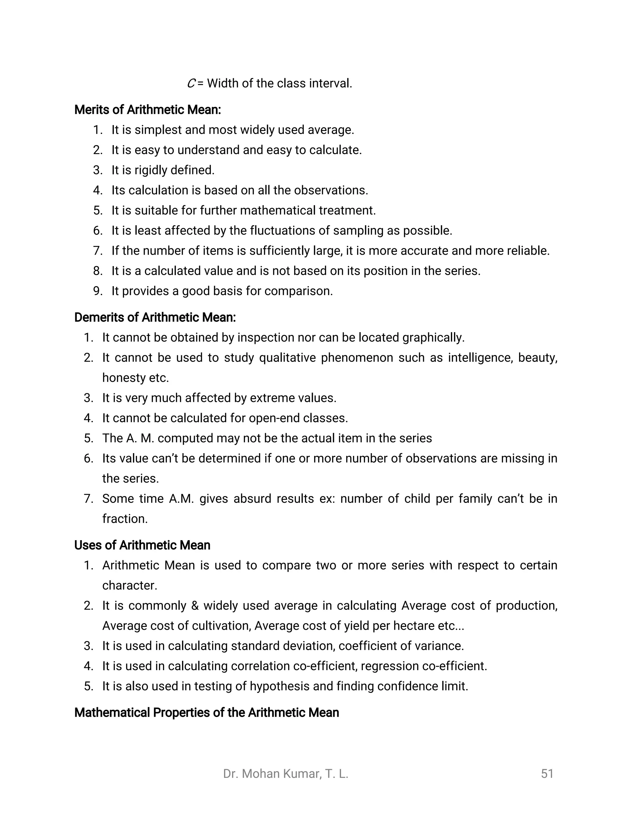
Chapter 15: Small Sample Tests:
15.1 Introductions:
The entire large sample theory was based on the application of “Normal test”.
The normal tests are based upon important assumptions of normality. But the
assumptions of normality do not hold good in the theory of small samples. If the
sample size “n” is small, the distribution of the various statistics (Z tests) are far from
normality and as such “Normal test” cannot be applied. Thus, a new technique is
needed to deal with the theory of small samples.
If the sample size is less than 30 (n < 30), then it is called small sample. For small
samples (n<30) generally we apply Student’s‘t’ test, ‘F-test and ‘Chi-square test’.
Independent Sample:
Two samples are said to be independent if the sample selected from one
population is not related to the sample selected from the second population.
Ex: a) Systolic blood pressures of 30 adult females and 30 adult males.
b) The yield samples from two varieties.
c) The soil samples are taken at different locations.
Dependent Sample:
Two samples are said to be dependent if each member of one sample corresponds
to a member of the other sample or if the observations in two samples are related.
Dependent samples are also called paired samples or matched samples.
Ex: a) The samples of nitrogen uptake by the top leaves and bottom
b) The yield samples from one variety before application of fertilizer and after
application of fertilizer.
c) Midterm and Final exam scores of 10 Statistic students.
Degrees of Freedom (df):
The number of independent variates which make up the statistic is known as the
degrees of freedom. Or
Degrees of freedom is defined as number of observations in a set minus number
of restrictions imposed on it. It is denoted by ‘df ‘
Suppose it is asked to write any four numbers then one will have all the numbers
of his choice. If a restriction is imposed to the choice is that the sum of these numbers
should be 50. Here, we have a choice to select any three numbers, say 10, 15, 20 and
the fourth number should be is 5 in order to make sum equals to 50: [50 - (10 +15+20)].

Thus our choice of freedom is reduced by one, on the condition that the total to be 50.
Therefore the restriction placed on the freedom is one and degree of freedom is three.
As the restrictions increase, the freedom is reduced.
15.2 Student’s ‘t’ test:
Student’s ‘t’ test was pioneered by W.S. Gosset (1908) who wrote under the pen
name of Student, and later on developed and extended by Prof. R.A. Fisher.
Let be the random sample of size ‘n’ form a normal population with a,x1 x2………xn
mean ‘µ’ and variance ‘σ2
’ then student’s t-test is defined by statistic
t = ~ df
- µ
̅
x
s
n
t (n -1)
where, and ; S is a unbiased estimate of population SD (σ). The=
̅
x
∑xi
n
S =
∑( -xi
̅
x )
2
n -1
above test statistic follows student’s t-distribution with (n-1) degrees of freedom.
15.3 Properties of t- distribution:
1. t-distribution ranges from - ∞ to ∞ just as does a normal distribution.
2. Like the normal distribution, t-distribution also symmetrical and has a mean zero.
3. t-distribution has a greater dispersion than the standard normal distribution.
4. As the sample size approaches 30, the t-distribution, approaches the Normal
distribution.
15.4 Assumptions:
1. The parent population from which the sample drawn is normal.
2. The sample observations are random and independent.
3. The population standard deviation σ is not known.
4. Size of the sample is small (i.e. n<30)
15.5 Applications of t-distribution or t-test
1) To test significant difference between sample mean and hypothetical value of
the population mean (single population mean).
2) To test whether any significant difference between two sample means.
i. Independent samples

ii. Related samples: paired t-test
3) To test the significance of an observed sample correlation co-efficient.
4) To test the significance of an observed sample regression co-efficient.
5) To test the significance of observed partial correlation co-efficient.
1) Test for single population means (one sample t- test)
Test procedure
Aim: To test whether any significant difference between sample mean and population
mean.
Let ‘µ’ is the population mean
‘ ’ is the sample mean
̅
x
‘S’ is the sample standard deviation
‘n’ is sample size
Steps:
1. Null Hypothesis H0: µ = µ0 i.e. There is no significant difference between sample
mean and population mean
H1: µ ≠ µ0 i.e. There is significant difference between sample mean and population
mean
H1: µ < µ0
H1: µ > µ0
2. Level of significance (α) = 5% or 1%
3. Consider test statistic : under Ho
t = ~ df
- µ
̅
x
s
n
t (n -1)
4. Compare the ‘tcal’ calculated value with the ‘ttab’ table value for (n-1) df at α level of
significance.
5. Determination of Significance and Decision
c. If |t cal| ≥ |t tab| for (n-1) df at α, Reject H0.
d. If |t cal| < |t tab| for (n-1) df at α, Accept H0.
6. Conclusion:

a. If we reject the null hypothesis conclusion will be there is significant difference
between sample mean and population mean.
b. If we accept the null hypothesis conclusion will be there is no significant
difference between sample mean and population mean.
2) Test of significance for difference between two means:
2a) Independent samples t-test:
If we want to test if two independent samples have been drawn from two normal
populations having the same means, the Standard deviation of two populations are
same and unknown.
Let x1, x2, …. xn1 and y1, y2,…… yn2 are two independent random samples from the
given normal populations. Let µ1 and µ2 are the mean of two populations, and
̅
x 1
̅
x 2
are mean of two samples, and are variance of two samples, and n1 and n2 are sizes2
1 s2
2
of two samples.
Test procedure
Aim: To test whether any significant difference between the two independent
samples mean.
Steps:
1. Null Hypothesis H0: µ1 = µ2 i. e. the samples have been drawn from the normal
populations with same means or both population have same mean
Alternative Hypothesis H1: µ1 ≠ µ2
2. Level of significance(α) = 5% or 1%
3. Consider test statistic: under H0
t = ~
-
̅
x 1
̅
y 2
S2
( +
1
n1
1
n2
)
t df(n1 + n2 – 2)
where, , and=
̅
x
∑xi
n1
=
̅
y
∑yi
n2
=S2
1
+ -2n1 n2
{ +∑( -xi
̅
x )
2
∑( -yi
̅
y )
2
}
4. Compare the ‘tcal’ calculated value with the ‘ttab’ table value for (n1 + n2 –2) df at α
level of significance.
a. If |t cal| ≥ t tab for (n1 + n2 – 2) df at α, Reject H0.
b. If |t cal| < t tab for (n1 + n2 – 2) df at α, Accept H0.

6. Conclusion
a. If we reject the null hypothesis conclusion will be there is significant
difference between the two sample means.
b. If we accept null hypothesis conclusion will be there is no significant
2b) Dependent or related samples or Paired t-test:
When n1 = n2 = n and the two samples are not independent but the sample
observations are paired together, then Paired t-test test is applied. The paired t-test is
generally used when measurements are taken from the same subject before and after
some manipulation/ treatment such as injection of a drug. For ex, you can use a
paired‘t’-test to determine the significance of a difference in blood pressure before and
after administration of an experimental presser substance.
You can also use a paired ‘t’-test to compare samples that are subjected to
different conditions, provided the samples in each pair are identical otherwise. For ex,
you might test the effectiveness of a water additive in reducing bacterial numbers by
sampling water from different sources and comparing bacterial counts in the treated
versus untreated water sample. Each different water source would give a different pair
of data points.
Assumptions/Conditions:
1. Samples are related with each other i.e. The sample observations (x1, x2 , ……..xn) and
(y1, y2,…….yn) are not completely independent but they are dependent in pairs.
2. Sizes of the samples are small and equal i.e., n1 = n2 = n(say),
3. Standard deviations in the populations are equal and not known
Test procedure
Let x1, x2………...xn are ‘n’ observations in first sample.
y1, y2………..yn are ‘n’ observations in second sample.
di = (xi - yi) = difference between paired observations.

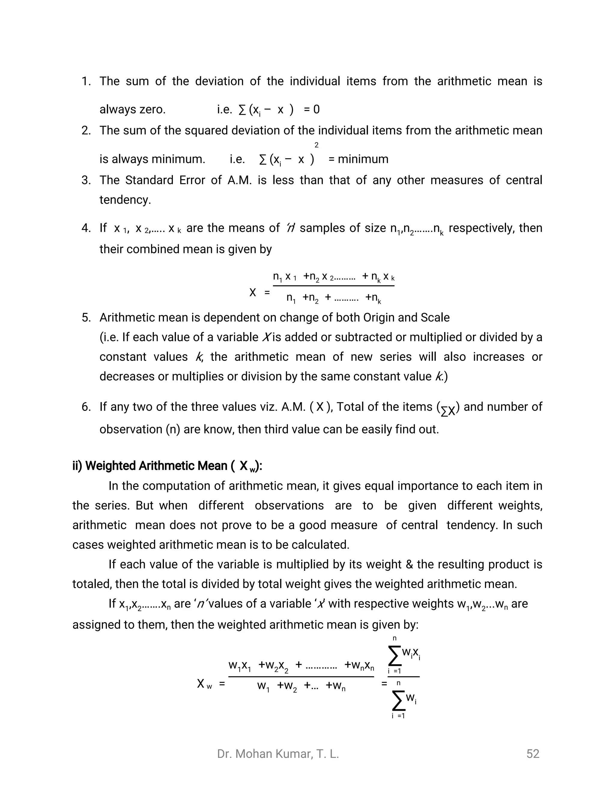
Steps:
1. H0: µ1 = µ2
H1: µ1 ≠ µ2
3. Consider test statistic: under H0
t = ~ df
⃓ ⃓
̅
d
s
n
t(n -1)
where, ; di=(xi-yi) = difference between paired observations and=
̅
d
∑di
n
S = 1
n -1[ -∑d2
( ∑d)
2
n ]
significance.
a. If |t cal| ≥ t tab for (n-1) df at α, Reject H0.
b. If |t cal| < t tab for (n-1) df at α, Accept H0.
6. Conclusion
a. If we reject the null hypothesis H0 conclusion will be there is significant difference
between the two sample means.
b. If we accept the null hypothesis H0 conclusion will be there no is a significant
15.6 Chi- Square Test ( test):χ2
The various tests of significance such that as Z-test, t-test, F-test have mostly
applicable to only quantitative data and based on the assumption that the samples were
drawn from normal population. Under this assumption the various statistics were
normally distributed. Since the procedure of testing the significance requires the
knowledge about the type of population or parameters of population from which
random samples have been drawn, these tests are known as parametric tests.
But there are many practical situations the assumption of about the distribution
of population or its parameter is not possible to make. The alternative technique where
no assumption about the distribution or about parameters of population is made are
known as non-parametric tests. Chi-square test is an example of the non-parametric

test and distribution free test.
Definition:
The Chi- square ( ) test (Chi-pronounced as ki) is one of the simplest and mostχ2
widely used non-parametric tests in statistical work. The test was first used by Karlχ2
Pearson in the year 1900. The quantity describes the magnitude of the discrepancyχ2
between theory and observation. It is defined as
= ~ dfχ2
∑[
( -oi Ei)2
Ei
] χ2
(n)
Where ‘O’ refers to the observed frequencies and ‘E’ refers to the expected frequencies.
Remarks:
1) If is zero, it means that the observed and expected frequencies coincide with eachχ2
other. The greater the discrepancy between the observed and expected frequencies the
greater is the value of .χ2
2) -test depends on only the on the set of observed and expected frequencies and on.χ2
degrees of freedom (df), it does not make any assumption regarding the parent
population from which the observation are drawn and it test statistic does not involves
any population parameter, it is termed as non-parametric test and distribution free test.
Measuremental data: The data obtained by actual measurement is called
measuremental data. For example, height, weight, age, income, area etc.,
Enumeration data: The data obtained by enumeration or counting is called enumeration
data. For example, number of blue flowers, number of intelligent boys, number of curled
leaves, etc.,
– test is used for enumeration data which generally relate to discrete variable whereχ2
as t-test and standard normal deviate tests are used for measure mental data which
generally relate to continuous variable.
Properties of Chi-square distribution:
1. The mean of distribution is equal to the number of degrees of freedom (n)χ2
2. The variance of distribution is equal to 2nχ2
3. The median of distribution divides, the area of the curve into two equal parts, eachχ2
part being 0.5.
4. The mode of distribution is equal to (n-2)χ2
5. Since Chi-square values always positive, the Chi square curve is always positively
skewed.

6. Since Chi-square values increase with the increase in the degrees of freedom, there is
a new Chi-square distribution with every increase in the number of degrees of
freedom.
7. The lowest value of Chi-square is zero and the highest value is infinity. i.e. Chi-square
ranges from 0 to ∞
Conditions for applying test:χ2
The following conditions should be satisfied before applying test.χ2
1. N, the total frequency should be reasonably large, say greater than 50.
2. No theoretical (expected) cell-frequency should be less than 5. If it is less than 5, the
frequencies should be pooled together in order to make it 5 or more than 5.
3. Sample observations for this test must be independent of each other.
4. test is wholly dependent on degrees of freedom.χ2
Applications of Chi-square distribution or Chi-square test
1. To test the goodness of fit
2. To test the independence of attributes.
3. To test the hypothetical value of population variance.
4. To test the homogeneity of population variance.
5. To test the homogeneity of independent estimates of population correlation
coefficient.
6. Testing of linkage in genetic problems.
1. Testing the Goodness of fit (Binomial and Poisson Distribution):
Karl Pearson developed a -test for testing the significance of the discrepancyχ2
between Actual (observed/experimental) frequency and the theoretical (expected)
frequency is known as goodness of fit.
In testing of hypothesis, our objective may be to test whether a sample has come
from a population that has a specified theoretical distribution like normal, binomial and
Poisson. In other words, it may be necessary to test whether an obtained frequency
distribution resembles a theoretical distribution. In plant genetics, our interest may be to
test whether the observed segregation ratios significantly from the Mendelian ratios. In
such situations we want to test the agreement between the observed and theoretical
frequencies such types of test is called as test of goodness of fit.
Under the null hypothesis (Ho) that there is no significant difference between the
observed and the theoretical values. Karl Pearson proved that the statistic

= ~χ2
n
∑i =1
[
( -oi Ei)2
Ei
] χ2
df(υ =n -k -1)
Follows -distribution with υ= n – k – 1 d.f. where O1, O2, ...On are the observedχ2
frequencies, E1 , E2…En, corresponding to the expected frequencies and k is the number
of parameters to be estimated from the given data. A test is done by comparing the
computed value with the table value of for the desired degrees of freedom.χ2
2. To test the independence of attributes - for m x n Contingency Table.
Let us consider the two attributes A and B, A is divided into m classes A1, A2, A3,...,
Am and B is divided into n classes B1, B2, B3,..., Bn. such a classification in which attributes
are divided into more than two classes is known as manifold classification. The various
cell frequencies can be expressed in the following table know as m*n manifold
contingency table. Where Oij denoted the cell which represents the number of person
possessing the both attributes Ai and Bj (i=1,2,3...,m; j=1,2,3...,n). Ri and Cj are
respectively called as ith
row total and jth
columns total (i=1,2,3..m and j=1,2,3..n) which
are called as marginal totals, and N is grand total.
Table 1: mxn Contingency table
Attribute
B
Attribute A
Row
Total
B1 B2 B3 .....
.
Am
A1 O11 O12 O13 ... Om3 R1
A2 O21 O22 O23 .... Om3 R2
A3 O31 O33 O33 ... Om3 R3
.
.
.
.
.
.
.
.
.
...
.
.
...
.
.
Am On1 On2 On3 Omn Rn
Col Total C1 C2 C3 .... Cm N

The table is to test if the two attributes A and B under consideration are
independent are not. The expected frequencies corresponding to any observed
frequency are calculated with the help of contingency table. The expected frequency Eij
corresponding to observed frequency Oij in the (i,j)th cell is calculated as
= =Eij
XRi Cj
N
Sum of ith row X Sum of jth column
size of sample
1 Null Hypothesis and Alternative Hypothesis
2 HO: The two factor or attributes are independent each other.
3 H1: The two factor or attributes are not independent each other.
4 Level of Significance is (( ) = 0.05 or 0.01
5 Test Statistic:
= ~χ2
m
∑i =1
n
∑j =1
( - )Oij Eij
2
Eij
χ2
(n -1)df(m -1)
6 If Compare the calculate the ‘ ’ value with the table value for df atχ2
cal χ2
tab (m -1)(n -1)
α level of significance .
5. Determination of significance and Decision
a. If ≥ for df at α, Reject H0.calχ2
tabχ2
(m -1)(n -1)
b. If < for df at α, Accept H0.calχ2
tabχ2
(m -1)(n -1)
6. Conclusion
a. If we reject the null hypothesis conclusion will be two factor or attributes are
independent each other.
b. If we accept the null hypothesis conclusion will be two factor or attributes are
not independent each other.
2.3 To test the independence of attributes- for 2X2 Contingency table:
Suppose the contingency table of order (2X2) for two factor A and B is presented
in below, then method of calculating from this will be easier and given as follows.χ2
Table2: 2x2 Contingency table
Attribute
B
Attribute B Row Total
A1 A2
B1 a b (a+b)= R1

B2 C d (c+d)= R2
Col Total (a+c)=C1 (b+d )=C2 a+b+c+d= N
The formula for finding from the observed frequencies a,b,c and d isχ2
= ~χ2
N(ad -bc)2
((c +d)(a +c)(b +d)(a +b)
χ2
1 df
The decision about independence of factor/attributes A and B is taken by comparing
with at certain level of significance; We reject or accept the null hypothesiscalχ2
tabχ2
accordingly at that level of significance.
Yate’ s Correction for Continuity
In a 2´2 contingency table, the number of df is (2-1)(2-1) =1. If any one of the
theoretical cell frequency is less than 5, the use of pooling method will result in df = 0
which is meaningless. In this case we apply a correction given by F. Yate (1934) which
is usually known as “Yates correction for continuity”. This consisting adding 0.5 to cell
frequency which is less than 5 and then adjusting for the remaining cell frequencies
accordingly. Thus corrected values of is given asχ2
=χ2
N[ -N/2]|ad -bc| 2
((c +d)(a +c)(b +d)(a +b)
F – Statistic Definition:
If X is a variate with n1 df and Y is an independent - variate with n2 df, then F- statisticχ2
χ2
is defined as i.e. F - statistic is the ratio of two independent chi-square variates divided
by their respective degrees of freedom. This statistic follows G.W. Snedocor’s
F-distribution with ( n1, n2) df i.e. F = ~
X
n1
Y
n2
F df(n1, n2)
Application of F-test:
1 Testing Equality/homogeneity of two population variances.
2 Testing of Significance of Equality of several means.
3 Testing of Significance of observed multiple correlation coefficients.
4 Testing of Significance of observed sample correlation ratio.
5 Testing of linearity of regression
1) Testing the Equality/homogeneity of two population variances:
Suppose we are interested to test whether the two normal populations have

same variance or not. Let x1, x2, x3 ….. xn1, be a random sample of size n1, from the first
population with variance and y1, y2, y3 … y n2, be random sample of size n2 form theσ1
2
second population with a variance . Obviously the two samples are independent.σ2
2
Null hypothesis:
i.e. population variances are same. In other words H0 is that the two=H0: =σσ1
2
2
2
σ2
independent estimates of the common population variance do not differ significantly.
i.e. population variances are different. In other words H1 is that the two≠H1: =σσ1
2
2
2
σ2
Independent estimates of the common population variance do differ significantly.
Calculation of test statistic:
Under H0, the test statistic is
F = ~
S2
1
S2
2
F df( ,ν1 ν2)
where, and=S2
1
1
-1n1
{∑( -xi
̅
x )
2
} =S2
2
1
-1n2
{∑( -yi
̅
y )
2
}
It should be noted that numerator is always greater than the denominator in F-ratio
F =
Larger variance
Smaller variance
n1 = =df for sample having larger variance-1n1
n2 = df for sample having smaller variance-1 =n2
The calculated value of Fcal is compared with the table value Ftab for n1 and n2 at
5% or 1% level of significance. If Fcal > Ftab then we reject Ho. On the other hand if Fcal <
Ftab we accept the null hypothesis and inferred that both the samples have come from
the population having same variance.
Since F- test is based on the ratio of variances it is also known as the Variance
Ratio test. The ratio of two variances follows a distribution called the F distribution
named after the famous statisticians R.A. Fisher.
Ranges
Between
Probability 0 to 1
Z statistic - ∞ to + ∞

t -statistic - ∞ to + ∞
Statisticχ2
0 to + ∞
F- statistic 0 to + ∞
Correlation -1 to +1
Regression - ∞ to + ∞
Binomial
variate
0 to n
Poisson
Variate
0 to + ∞
Normal Variate - ∞ to + ∞

Chapter 16: CORRELATION
16.1 Introduction
The term correlation is used by a common man without knowing that he is
making use of the term correlation. For example when parents advice their children to
work hard so that they may get good marks, they are correlating good marks with hard
work. Sometimes the variables may be inter-related. The nature and strength of
relationship may be examined by correlation and Regression analysis.
16.2 Definition:
Correlation is a technique/device//tool to measure the nature and extent of
relationship of two or more variables.
Ex: Study the relationship between blood pressure and age, consumption level of
nutrient and weight gain, total income and medical expenditure, relation between height
of father and son, yield and rainfall, wage and price index, share and debentures etc.
Correlation is statistical analysis which measures nature and degree of
association or relationship between two or more variables. The word association or
relationship is important. It indicates that there is some connection between the
variables. It measures the closeness of the relationship. Correlation does not indicate
cause and effect relationship.
16.3 Uses of correlation:
1) It is used in physical and social sciences.
2) It is useful for economists to study the relationship between variables like price,
quantity etc.. for businessmen estimates costs, sales, price etc. using
correlation.
3) It is helpful in measuring the degree of relationship between the variables like
income and expenditure, price and supply, supply and demand etc…
4) It is the basis for the concept of regression.
16.4 Types of Correlation:
i) Positive, Negative and No Correlation
ii) Simple, Multiple, and Partial Correlation
iii) Linear and Non-linear
iv) Nonsense and Spurious Correlation
i) Positive, Negative, and No Correlation:

These depend upon the direction/movement of change of the variables.
Positive or direct correlation
If the two variables tend to move together in the same direction, i.e. an increase
in the value of one variable is accompanied by an increase in the value of the other (↑↑)
or decrease in the value of one variable is accompanied by a decrease in the value of
other (↓↓), then the correlation is called positive or direct correlation.
Ex: Price and supply, height and weight, yield and rainfall, Height and weight of a
person, Number of pods and yield of a crop are some examples of positive correlation.
Negative (or) indirect or inverse correlation.
If the two variables tend to move together in opposite directions, i.e. increase (or)
decrease in the value of one variable (↑↓) is accompanied by a decrease or increase in
the value of the other variable (↓↑), then the correlation is called negative (or) indirect or
inverse correlation.
Ex: Price and Quantity demanded, yield of crop and drought, pest attack and yield,
Disease and yield are examples of negative correlation.
Uncorrelation/ No Correlation/Zero Correlation
If there is no relationship between the two variables such that the value of one
variable change and the other variable remain constant is called no or zero correlation.
ii) Simple, Multiple and Partial Correlations:
In case of simple correlation, there are only two variables under consideration
Ex: money supply and price level.
In case of Multiple Correlation, the relationship between more than two variables
is considered; here three or more variables are studied simultaneously.
Ex: the relationship of price, demand and supply of a commodity are studies at a
time.

Partial correlation involves studying the relationship between two variables after
excluding the effect of one or more variables.
Ex: study of partial correlation between price and demand would involve studying
the relationship between price and demand excluding the effect of money supply,
exports, etc.
iii) Linear and Nonlinear correlation:
If the change in one variable is accompanied by change in another variable in a
constant ratio, then there will be linear correlation between them. Here the ratio of
change between the two variables is the same. If we plot these variables on graph
paper, all the points will fall on the same straight line.
If the amount of change in one variable not bear change in the another variable at
constant ratio. Then the relation is called Curvi-linear (or) non-linear correlation. The
graph will be a curve.
iv) Nonsense or Spurious Correlation:
Nonsense correlation is a correlation supported by data but having no basis in
reality. Or A false presumption is that two variables are correlated but in reality they are
not at all correlated.
Ex: Correlation between incidence of common cold and ownership of television.
The correlation, between the size of shoe and the intelligence of a group of
individuals.
Spurious correlation is the correlation between two variables that does not result
from any direct relation between them but from their relation to other variables.
16.5 Univariate data and Bivariate data:
The data on a single variable over a given set of object is called univariate data.
Ex: Yield on different plants.
The data on two variables over a given set of objects is called bivariate data.

Ex: Yield and disease intensity on different plants. The variables are yield and
disease intensity. The objects are plants.
16.6 Variance and Co-Variance:
The unknown variation affecting univariate data is measured by standard
deviation. Square of the standard deviation is called variance. Variance of a variable X is
denoted by V(X).
The unknown variation affecting the bivariate is measured by co-variance.
Co-variance of the variables X and Y is denoted by Cov (X, Y).
Co-variation:
The co-variation between the variables x and y is defined as
Cov =( x,y)
∑ (y - )(x -
̅
x ) ̅
y
n
where , are respectively means of X and Y and ‘ n’ is the number of pairs of
̅
x
̅
y
observations.
16.7 Method of measurement of Correlation
When there exist some relationship between two variables, we have to measure
of the degree of relationship between them. This measure is called the measure of
correlation (or) correlation coefficient and it is denoted by ‘r’.
Correlation can be measured using following methods
1) Scatter diagram or Dot diagram or Scattergram.
3) Product Moment or Co-variance or Karl Pearson’s coefficient of correlation
4) Spearman’s Rank Correlation
1) Scatter Diagram:
This method is also known as Dotogram or Dot diagram. It is the simplest
method of studying the relationship between two variables diagrammatically. One
variable is represented along the horizontal axis and the second variable along the
vertical axis. For each pair of observations of two variables, we put a dot in the plane.
There are as many dots in the plane as the number of paired observations of two
variables. The diagram so obtained is called "Scatter Diagram". By studying diagram, we

can have rough idea about the nature and degree of relationship between two variables.
The term scatter refers to the spreading of dots on the graph.
The direction of dots shows the scatter or concentration of various points. This
will show the type of correlation or degree of correlations.
1) If all the plotted points form a straight line from lower left hand corner to the upper
right hand corner then there is Perfect positive correlation. We denote this as r = +1
2) If the plotted points in fall in a narrowband and they show a rising trend from the
lower left hand corner to the upper right hand corner the two variables are highly
positively correlated. In this case the coefficient of correlation takes the value 0.5 < r
<0.9.
3) If the plotted points fall in a loose band from the lower left hand corner to the upper
right hand corner, there will be a low degree of positive correlation. In this case the
coefficient of correlation takes the value 0< r < 0.5.
4) If the plotted points in the plane are spread all over the diagram there is no
correlation between the two variables. Here r=0.
5) If the plotted points fall in a loose band from the upper left hand corner to the lower
right hand corner, there will be a low degree of negative correlation. In this case the
coefficient of correlation takes the value -0< r < -0.5.
6) If the plotted points fall in a narrowband from the upper left hand corner to the lower
right hand corner, there will be a high degree of negative correlation. In this case the
coefficient of correlation takes the value -0.5 < r < -0.9.
7) If all the plotted dots lie on a straight line falling from upper left hand corner to lower
right hand corner, there is a perfect negative correlation between the two variables. In
this case the coefficient of correlation takes the value r = -1.
2) Karl Pearson’s coefficient of correlation:
A mathematical method for measuring the intensity or the magnitude of linear
relationship between two variables was suggested by Karl Pearson (1867-1936), a great

British Biometrician and Statistician and, it is most widely used method in practice.
Karl Pearson’s measure, known as Pearsonian correlation coefficient between
two variables X and Y, usually denoted by r(X,Y) or rxy or simply r is a numerical measure
of linear relationship between them. It is defined as the ratio of the covariance between
X and Y, to the product of the standard deviations of X and Y.
Symbolically:
If ( x1, y1), (x2, y2);( x3, y3);..................(xn, yn) are n pairs of observations of the variables X
and Y in a bivariate distribution, sX and sY are S.D of X and Y respectively. Then
Correlation coefficient (r ) given by;
=rxy
Cov (X,Y)
σX σY
Or
r =
Cov (X, Y)
V .V(Y)(X)
where, X and Y → variables
→ covariance between X and YCov =(X,Y)
1
n
∑ ( -xi
̅
x )( -yi
̅
y )
→ variance of XV =(X)
1
n
∑( -xi
̅
x )
2
→ variance of YV =(Y)
1
n
∑( -yi
̅
y )
2
Then the correlation coefficient is given by
=rxy
∑( -xi
̅
x )( -yi
̅
y )
∑( -xi
̅
x )
2
∑( -yi
̅
y )
2
we can further simply the calculations, then Pearsonian correlation coefficient given as
=rxy
-
∑XY
∑X∑Y
n
∑ -X2
(∑X)
2
n
∑ -Y2
(∑Y)
2
n
Or

= =rxy
n -∑XY ∑X∑Y
n∑ -X2
(∑X)
2
n∑ -Y2
(∑Y)
2
n -∑XY ∑X∑Y
{n∑ -X2
(∑X)
2
}{n∑ -Y2
(∑Y)
2
}
In the above method we need not find mean or standard deviation of variables
separately. However, if X and Y assume large values, the calculation is again quite time
consuming.
Remarks:
The denominator in the above formulas is always positive. The numerator may
be positive or negative; therefore the sign of correlation coefficient (r) will be decided by
either positive or negative sign of Cov(X, Y).
Assumptions of Pearsonian correlation coefficient (r):
Correlation coefficient r is used under certain assumptions, they are
1. The variables under study are continuous random variables and they are normally
distributed
2. The relationship between the variables is linear
3. Each pair of observations is unconnected with other pair (independent)
Interpreting the value of ‘r’:
The following table sums up the degrees of correlation corresponding to various
values of Pearsonian correlation coefficient (r):
Degree of Correlation Positive Negative
Perfect Correlation +1 -1
Very high degree of correlation > +0.9 > -0.9
Sufficiently high degree of correlation +0.75 to +0.9 -0.75 to -0.9
Moderate degree of correlation +0.6 to +0.75 -0.6 to -0.75
Only possibility of correlation +0.3 to +0.6 -0.3 to -0.6
Possibly no correlation < +0.3 < -0.3
No correlation 0 0
Properties of Pearsonian correlation coefficients:

1. The correlation coefficient value ranges between –1 and +1.
2. The correlation coefficient is independent of both change of origin and scale.
3. Two independent variables are uncorrelated but the converse is not true
4. The Pearsonian coefficient of correlation is the geometric mean of the two
regression coefficients i.e. =rxy byx bxy
5. The square of Pearsonian correlation coefficient is known as the coefficient of
determination.
6. The correlation coefficient of x and y is symmetric. i.e.rxy = ryx.
7. The sign of correlation coefficient depends on the only sign of Covariance between
two variables
8. It is a pure number independent of units of measurement.
Remarks:
3) One should not be confused with the words uncorrelation (no correlation) and
independence. If rxy = 0 means uncorrelation between the variables X and Y simply
implies the absence of any linear (straight line) relationship between them. They
may, however, be related in some other form other than straight line e.g., quadratic,
cubic, polynomial, logarithmic or trigonometric form.
3) Spearman’s Rank Correlation
Sometimes we come across statistical series in which the variables under
consideration are not capable of quantitative measurement but can be arranged in
serial order. This happens when we are dealing with qualitative characteristics
(attributes) such as honesty, beauty, character, morality, etc., which cannot be
measured quantitatively but can be arranged serially. In such situations Karl Pearson’s
coefficient of correlation cannot be used as such.
Charles Edward Spearman, a British Psychologist, developed a formula in 1904,
which consists in obtaining the correlation coefficient between the ranks of n
individuals in the two attributes under study.
Suppose we want to find if two characteristics A, say, intelligence and B, say,
beauty are related or not. Both the characteristics are incapable of quantitative
measurements but we can arrange a group of N individuals in order of merit (ranks)
w.r.t. proficiency in the two characteristics. Let the random variables X and Y denote the
ranks of the individuals in the characteristics A and B respectively. If we assume that
there is no tie, i.e., if no two individuals get the same rank in a characteristic then,

obviously, X and Y assume numerical values ranging from 1 to n.
The Pearsonian correlation coefficient between the ranks of two qualitative
variables (attributes) X and Y is called the rank correlation coefficient.
Spearman’s rank correlation coefficient, usually denoted by ρ (Rho) is given by the
equation
ρ =1 -
6∑d2
i
n( -1n2
)
where, difference between the pair of ranks of the same individual in the=di ( -xi yi)
two characteristics and n is the number of pairs of observations.
Repeated values/tied observations:
In case of attributes if there is a tie in values i.e., if any two or more individuals
are placed with the same value w.r.t. an attribute, then Spearman’s for calculating the
rank correlation coefficient breaks down. In this case common ranks are assigned to
the repeated values (observations). For example if the value so is repeated twice at the
5th rank, the common rank to be assigned to each item is (5+6)/2=5.5, which is the
average of 5 and 6 given as 5.5, appeared twice. These common ranks are the
arithmetic mean of the ranks, assigned to tied observation and the next item will get the
rank next to the rank used in computing the common rank.
Then the Spearman’s rank correlation formula it is required to apply a correction factor
which uses a slightly different formula given by:
ρ =1 -
6 +c.f}{∑d2
i
n( -1n2
)
Where, c.f. = Correction factor
c.f. =
∑( - )m3
i mi
12
Number of times the value is repeated/tied=mi
Remarks on Spearman’s Rank Correlation Coefficient
1. Rank correlation co-efficient lies between -1 and +1. i.e. Spearman’s-1 ≤ ρ ≤ +1.
rank correlation coefficient, ρ, is nothing but Karl Pearson’s correlation coefficient (r)
between the ranks; it can be interpreted in the same way as the Karl Pearson’s
correlation coefficient.

2. Karl Pearson’s correlation coefficient assumes that the parent population from which
sample observations are drawn is normal. If this assumption is violated then we
need a measure, which is distribution free (or non-parametric). Spearman’s ρ is such
a distribution free and nonparametric measure, since no strict assumptions are
made about from of the population from which sample observations are drawn.
3. Spearman’s formula is the only formula to be used for finding correlation coefficient
if we are dealing with qualitative characteristics, which cannot be measured
quantitatively but can be arranged serially. It can also be used where actual data are
given.
4. Spearman’s rank correlation can also be used even if we are dealing with variables,
which are measured quantitatively, i.e. when the actual data but not the ranks relating
to two variables are given. In such a case we shall have to convert the data into
ranks. The highest (or the smallest) observation is given the rank 1. The next highest
(or the next lowest) observation is given rank 2 and so on. It is immaterial in which
way (descending or ascending) the ranks are assigned.

16.8 To test the significance of an observed sample correlation co-efficient
Test procedure
Aim: To test whether any significant correlation between two variables.
Steps:
1. H0 : There is no significant correlation between two variables. i.e. ρ = 0
H1: There is a significant correlation between two variables. i.e. ρ ≠ 0
3. Consider test statistic: under Ho
t = ~ df
r
1 -r2
n -2 t(n -2)
where ‘r’ is observed correlation co-efficient and ρ is population correlation
co-efficient
significance.
e. If |t cal| ≥ t tab for (n-2) df at α, Reject H0.
f. If |t cal| < t tab for (n-2) df at α, Accept H0.
6. Conclusion
a) If we reject the null hypothesis, conclusion will be there is significant correlation
between two variables.
b) If we accept the null hypothesis conclusion will be there is no significant
correlation between two variables.

Chapter 17.: Regression Analysis
17.1 Introduction:
In correlation analysis, we have studied the nature of relationship between two or
more variable which are closely related to each other by their degree of relationship.
After knowing the relationship between two variables researcher interested to know its
magnitude and the fact that which variable affecting the other variable i.e. cause and
effect relationship between to variable, which can’t be studied using correlation. By
knowing cause and effect relationship, we may interested in estimating (predicting) the
value of one variable given the value of another. The variable representing cause is
known as independent variable and is denoted by X. The variable representing effect is
known as dependent variable and is denoted by Y. In other words, the variable predicted
on the basis of other variables is called the dependent and the other is the independent
variable. In regression analysis independent variable is also known as regressors or
predictor or explanatory variable, while dependent variable is also known as regressed
or predicted or explained or response variable.
“The relationship between the dependent and the independent variable may be
expressed as a function and such functional relationship is termed as regression”.
The relationship between two variables can be considered between, say, rainfall
and agricultural production, price of an input and the overall cost of product, consumer
expenditure and disposable income. Thus, regression analysis reveals average
relationship between two variables and this makes possible estimation or prediction.
The term regression literally means “Return back” or “Moving back” or “Stepping
back towards the average”. It was first used by a British Biometrician Sir Francis Galton
in 1887 in the study of heredity. He reported his discovery that sizes of seeds of pea
plants appeared to “revert” or “regress”, to the mean size in successive generations. He
also studied the relationship between heights of fathers and heights of their sons and
conclude that “An average height of tall father have short sons, and shorter father have
tall sons”
Definition: Regression is the measure of the average relationship between two or more
variables in terms of the original units of the data.
17. 2 Application of Regression Analysis:
1) It helps to establish functional or causal relationship between two or more
variables.

2) Once functional relationship between two or more variables are established. It can
be used to predict the unknown values of dependent variable on the basis of known
value of independent variable.
3) To know the amount of change in the dependent variable for unit change in
independent variable.
4) Regression analysis widely used in statistical estimation of demand curve, supply
curves, production curves, cost function, consumption function etc...
17.3 Types of Regression:
The regression analysis can be classified into:
1) Simple, Multiple and Partial regression
2) Linear and Nonlinear regression
1) Simple, Multiple and Partial regression:
When there are only two variables, the functional relationship is known as simple
regression. One is dependent variable another is independent variable. Ex: yield of a
crop (Y) and the length of panicles (X) are considered. Model is Y=f(X)
When there are more than two variables and one of the variables is dependent
upon others, then the functional relationship is known as multiple regression. Ex: yield
of a crop (Y) may depends the length of panicles (X1), number of grains per panicle (X2)
and number of leaves (X3) are considered. Model is Y=f(X1, X2, X3).
In the case of partial relationship one or more variables are considered, but not
all by excluding the influence of some of variable. Example yield of a crop (Y), the length
of panicles (X1), number of grains per panicle (X2) and number of leaves (X3) are
considered then regression equation be Y= f (X1, but excluding effect of X2 and X3)
Y= f (X2, but excluding effect of X1 and X3)
Y= f (X3, but excluding effect of X1 and X2)
2) Linear and Nonlinear regression
If the relationship between two variables is a straight line, it is known as simple
linear regression. In this case the regression equation will be a function of only first
order/ degree. Equation of linear regression is a straight line equation given by Y=a+bX.
But, remember a linear relationship can be both simple and multiple.
If the regression equation/curve between two or more variables is not a straight
line, the regression is known as curved or nonlinear regression. In this case the
regression equation will be a function of higher order of type X2
, XY, X3
etc..

Nonlinear Regression equation are 1)Y=a+bX2
, 2) Y=a+bX3
, 3) Y=a+bXY etc..
17.4 Simple Linear Regression:
If we consider linear regression of two variables Y and X, we shall have two
regression lines namely Y on X and X on Y. The two regression lines show the average
relationship between the two variables.
The regression line is the graphical or relationship representation of the best
estimate of one variable for any given value of the other variable.
1) Regression line Y on X is a line that gives best estimate of Y for given value of X. Here
Y is dependent and X is independent
2) Regression line of X on Y is a line that gives the best estimate of X for given value of
Y. Here X is dependent and Y is independent.
Again, these regression lines are based on two equations known as regression
equations. These equations show best estimate of one variable for the known value of
the other.
1) Linear regression equation of Y on X is Y = a + bX
2) Linear regression equation X on Y is X = a + bY
1) The Regression Equation of Y on X:
The regression equation of Y on X is given as
Y = a +bX +e
Where
Y= dependent variable;
X = independent variable
a = intercept
b = the regression coefficient (or slope) of the line.
e = error
“a” and “b” are called as constants
The constants “a” and “b” can be estimated with by applying the “Least Squares
Principle”. This involves minimizing . This gives=∑e2
∑(Y -a -bX)2
b = =byx
Cov (X,Y)
V(X)

=byx
-
∑XY
∑X∑Y
n
∑ -X2
(∑X)
2
n
Or
=byx
n -∑XY ∑X∑Y
n∑ -X2
(∑X)
2
and a = -
̅
Y byx
̅
X
where is called the estimate of regression coefficient of Y on X and it measures thebyx
change in Y for a unit change in X.
The fitted regression equation of Y on X for predicting of unknown value of Y
from know value of X is given by
= + X
̂
Y
̂
a
̂
b yx
2) The regression equation of X on Y: Simply by replacing X with Y, and Y with X in the
regression equation Y on X, we get the regression equation of X on Y
The regression equation of X on Y is given as
X = + Y +(a'
b'
Where
X= dependent variable;
Y = independent variable
a' = intercept (or Mean) of the line
b' = the regression coefficient (or slope) of the line.
= error(
a' and b' are also called as constants
The constants a' and b' can be estimated with by applying the “least squares method”.
This involves minimizing . This gives=∑(2
∑(X - - Ya'
b'
)2
=bxy
n -∑XY ∑X∑Y
n∑ -Y2
(∑Y)
2
and = -a'
̅
X bxy
̅
Y

where is called the estimate of regression coefficient of X on Y and it measures thebxy
change in X for a unit change in Y.
The fitted regression equation of X on Y for predicting of unknown value of X
from know value of Y is given by
= + Y
̂
X
̂
a
̂
b xy
Interpretation of Regression Co-efficient Y on X is :byx
Regression Co-efficient is a measure of change in the value of dependent
variable (Y) for corresponding unit change in the value of independent variable (X). It is
also called slope of the regression line Y on X.
Interpretation of Regression Co-efficient X on Y is :bxy
Regression Co-efficient is a measure of change in the value of dependent
variable (X) for corresponding unit change in the value of independent variable (Y). It is
also called slope of the regression line X on Y.
Note: Population regression co-efficient is denoted by ‘βyx’ or ‘βxy’
Sample regression co-efficient is denoted by ‘ ’ or ‘ ’byx bxy
17.6 Properties of Regression coefficients:
1) The range of regression coefficient is -( to +(.
2) The correlation coefficient is the geometric mean of the two regression
coefficients
i.e. =rxy byx bxy
3) Regression coefficients are independent of change of origin but not of scale.
4) If one of the regression coefficients is greater than unity, the other must be less
than unity.
i.e. >1 ⇔ <1byx bxy
5) The sign of the correlation coefficient and regression coefficients will be always
same.
i.e. = +ve⟺ = +vebyx ryx
= -ve⟺ = -vebyx ryx
6) Both regression coefficients must have the same sign, i.e. either theyandbyx bxy
will be positive or negative.
7) The two regression coefficients are not symmetric. i.e.andbyx bxy ≠ .byx bxy
8) Units of regression coefficients are same as that of the dependent variable.

9) Arithmetic mean of two regression coefficients is equal to or greaterandbyx bxy
than the coefficient of correlation.
i.e. ≥r
+byx bxy
2
10) If two variable X and Y are independent, then regression and correlation
coefficient is Zero
11)Both the lines regression pass through the point ( ). In other words, the mean,
̅
X
̅
Y
values ( ) can be obtained as the point of intersection of the two regression,
̅
X
̅
Y
lines.
17.7 Difference between Correlation and Regression:
Sl.no. Correlation Regression
1. Correlation is the nature or degree of
relationship between two or more
variables. Where the change in one
variable affects a change in other
variable
Regression is mathematical measure of the
average relationship between two or more
variables. Where one variable is dependent
and other variable is independent
2. It is two way relationship It is one way relationship.
3. The correlation coefficient of X and X is
symmetric. i.e. rxy = ryx
Regression coefficients are not symmetric in
X and Y, i.e., byx ≠ bxy.
4. Correlation need not imply cause and
effect relationship between the variable.
Regression analysis clearly indicates the
cause and effect relationship between the
variables.
5. There is no prediction of variables. There is a prediction of one variable for other
variable.
6. The correlation coefficient is
independent of both change of origin
and scale.
Regression coefficients are independent of
change of origin but not of scale.
7. Range is -1 to +1 Range is -∞ to +∞
8. Correlation coefficient relative measure
of linear relationship between X and Y.
Regression coefficient is absolute measures.
9. It is pure number, independent of units It is expressed in the units of dependent

of measurements. variable
10. The Correlation Co-efficient is denoted
by
‘ρ’ for population
‘r’ for sample
Regression Co-efficient is denoted by
‘β’ population
‘b’ sample

17.8 The relationship between regression coefficient and correlation coefficient:
The regression coefficient is given by
b = = = (1)byx
Cov (X,Y)
V(X)
Cov (X,Y)
σ2
x
The correlation coefficient is given by
r =
Cov (X,Y)
σX σY
It can be written as (2)Cov =r(X,Y) σX σY
By substituting eqn. (2) in (1) we get, =byx
r σX σY
σ2
x
After simplification we get
Similarly
Where r is correlation coefficient, and are S.D. of X and Y respectivelyσX σY
17.9 Regression Lines and Coefficient of Correlation
=rbxy
σX
σY
=rbyx
σY
σX

1) In case of perfect positive correlation (r = +1) and in case of perfect negative
correlation (r = -1) the two regression lines will coincide (parallel to each other),
i.e. we have only one straight line, see Figure (a) and (b)
2) The angle between two regression lines small, then the degree of correlation will
be more, see Figure (c) and (d).
3) The angle between two regression lines is more, then lesser will be the degree of
correlation, see Figure (e) and (f).
4) If the variables are independent i.e. No Correlation (r = 0), the two regression
lines are perpendicular to each other See Figure (g)
17.11 Test of significance of regression co-efficient
Test procedure
1. H0: Regression co-efficient is not significant. i.e. b = 0
H1: Regression co-efficient is significant. i.e. b ≠ 0
3. Consider test statistic
t = ~ df
̂
b
SE(b)
t(n -2)
where, ,=r
̂
b
Sy
Sx SE =(b)
-S2
y b2
S2
x
(n -2)S2
x
4. Compare the calculate the ‘t’ value with the table ‘t’ value for (n-2) df at α level of

significance .
5. Determination of significance and Decision
a. If |t cal | ≥ t tab for (n-2) df at α, Reject H0.
b. If |t cal | < t tab for (n-2) df at α, Accept H0.
6. Conclusion
a. If we reject the null hypothesis conclusion will be regression co-efficient is
significant.
b. If we accept the null hypothesis conclusion will be regression co-efficient is
not significant.

Chapter 18.: Analysis of Variance (ANOVA)
18.1 Introduction:
The analysis of variance is a powerful statistical tool for tests of significance of
several populations mean. The term Analysis of Variance was introduced by Prof. R.A.
Fisher to deal with problems in agricultural research.
The test of significance based on Z-test and t-test are only an adequate
procedure for testing the significance of one or two sample means. In some situation,
three or more population mean to be consider at a time for testing. Therefore, an
alternative procedure is needed for testing these means. For ex: five fertilizers are
applied to four plots of wheat and its yield on each of the plot is given. We may be
interested in finding out whether the effect of these fertilizers on the yields is
significantly different i.e. all the fertilizers application on wheat plot gives same yield or
different yield. Answer of this problem is provided by the technique of analysis of
variance. Thus basic purpose of the analysis of variance is to test the equality of several
means.
Variation is inherent in nature. The total variation in any set of numerical data is
due to a number of causes which may be classified as: (i) Assignable causes and (ii)
Chance causes. The variation due to assignable causes can be detected and measured,
whereas the variation due to chance causes is beyond the control of human hand and
cannot be traced separately.
Definition of ANOVA:
The analysis of variance is the systematic algebraic procedure of decomposing (i.e.
partitioning) overall variation ( i.e. total variation) in the responses observed in an
experiment into different component of variations such as treatment variation and error
variation. Each component is attributed identifiable cause or source of variation.
18.2 Assumptions of ANOVA:
For the validity of the F-test in ANOVA the following assumptions are made.
1. The effects of different factors (treatments and environmental effects) are additive
in nature.
2. The observations and experimental errors are independent
3. Experimental errors are distributed independently and normally with mean zero and
constant variation i.e. )ε~N(0, σ2

4. Observations of character under study follow normal distribution
18.3 One-way Classification: (One-way ANOVA)
Suppose, n observations of random variable yij ,( i = 1, 2, …… k ; j = 1,2….ni) are
grouped into ‘k’ classes of sizes n1, n2 , …..nk respectively ( as given in belown = )∑k
i =1
ni
table.
The total variation in the observation Yij can be split into the following two
components:
1) The variation between the classes, commonly known as treatment variation/class
variation.
2) The variation within the classes i.e., the inherent variation of the random variable
within the observations of a class.
The first type of variation is due to assignable causes, which can be detected and
controlled by human endeavor and the second type of variation due to chance causes
which are beyond the control of human.
Classes/grou
ps
Total Mean
1 y11 y12 y13 ... y1n1 T1
=
̅
Y 1
T1
n1
2 y21 y22 y23 ... y2n2 T2
=
̅
Y 2
T2
n2
3 y31 y32 y31 ... y3n3 T3
=
̅
Y 3
T3
n3
: : : : :.... : : :
k yk1 yk2 yk3 ... yknk Tk
=
̅
Y k
Tk
nk
Grand total
(GT)
Grand Mean
( )
̅
Y
Test Procedure: The steps involved in carrying out the analysis are:
1) Null Hypothesis (H0): H0: (1 = (2 = …= (k=(
Alternative Hypothesis (H1): all (i’s are not equal (i = 1,2,…,k)
2) Level of significance (( ): Let ( = 0.05 or 0.01
3) Computation of test statistic: steps
Various sums of squares are obtained as follows.
a) Find the sum of values of all the items ( of the given data. Let this grandn = )∑k
i =1
ni

total represented by ‘GT’.
b) Then correction factor (C.F.) =
(GT)2
n
c) Find Total sum of squares (TSS): TSS = -(C.F.)∑k
i =1∑ni
j =1
y2
ij
d) Find sum of squares between the classes or between the treatments (SSTr) is
SSTr = -∑k
i =1
T2
i
ni
(C.F.)
Where ni (i: 1,2,…..k) is the number of observations in the ith
class.
e) Find the sum of squares within the class or sum of squares due to error (SSE):
SSE = TSS - SSTr
ANOVA Table:
Sources of Variation d.f Sum of squares
(S.S.)
M.S.S F
ratio
Between treatments k-1 SSTr MST=
SSTr/k-1
MST
MSE
Within treatment
(Error)
N-
k
SSE MSE=
SSE/N-k
Total N-
1
TSS
Test Statistic: Under Ho
= = ( F(k -1, N -k)Fcal
Variance between the treatments
Variance within the treatment
MST
MSE
4) Critical value of F or Table value of F:
The table value is obtained from F-table for (k-1, N-k) df at ( % & denoted it as Ftab.
5) Decision criteria:
If Fcal ( Ftab,( Reject Ho and concluded that the class means or treatment means are
significantly different ( i.e. class means are not same).
If Fcal < Ftab, ( Accept Ho and concluded that the class means or treatment means
are not significantly different (i.e. class means are not equal).
18.4 Two-way Classification: (Two-way ANOVA):
Let us consider the case when there are two factors which may affect the variate
yij values under study Ex: The yield of cow milk may be affected by rations (feeds) as
well as the varieties (breeds) of the cows. Let us now suppose that the n cows are

divided into ‘h’ different groups or classes according to their breed, each group
containing ‘k’ cows and then let us consider the effect of k treatments (rations) given at
random to cows in each group on the yield of milk.
Let the suffix ‘i’ refer to the treatments (rations/feeds) and ‘j’ refer to the varieties
(breed of the cow), then the yields of milk is yij (i:1,2, …..k; j:1,2….h) of n (= R(C) cows
furnish the data for the comparison of the treatments (rations) as well as varieties. The
yields may be expressed as variate values in the following k( h two way table.
Ration
s
Breeds Total Mean
1 2 3 j h
1 y11 y12 y13 ... y1h R1
.
̅
y 1
2 y21 y22 y23 ... y2h R2
̅
y 2.
3 y31 y32 y31 ... y3h R3
̅
y 3.
i : : : yij : : :
k yk1 yk2 yk3 ... ykh Rk
̅
y k.
Total C1 C2 C3 Cj Ch Grand total
(GT)
Mean ̅
y .1
̅
y .2
̅
y .3
̅
y .j
̅
y .h
Grand Mean
( )
̅
Y
The total variation in the observation yij can be split into the following three
components:
(i) The variation between the treatments (rations)
(ii) The variation between the varieties (breeds)
(iii) The inherent variation within the observations of treatments and varieties.
The first two types of variations are due to assignable causes which can be
detected and controlled by human endeavor and the third type of variation due to
chance causes which are beyond the control of human hand.
Test procedure for two -way analysis: The steps involved in carrying out the analysis
are:
1. Null hypothesis (Ho):
Ho : (1. = (2. = ……(k. = (. (for comparison of treatment/ rations) i.e., there is no
significant difference between rations (treatments)
H1:(.1 = (.2 = …(.h = m.(for comparison of varieties/ breed and stock) i.e. there is no

significant difference betweenvarieties ( breeds)
2. Level of significance ((): 5% or 1%
3. Test Statistic:
1) Find the sum of values of all n (=k(h) items of the given data.
Let this grand total represented by ‘GT ’.
Then correction factor (C.F.) =
(GT)2
N
2) Find the total sum of squares (TSS) TSS = -(C.F.)∑k
i =1∑h
j =1
y2
ij
3) Find the sum of squares between treatments or sum of squares between rows is
SSTr =SSR = -∑k
i =1
R2
i
h
(C.F.)
where ‘h’ is the number of observations in each row
4) Find the sum of squares between varieties or sum of squares between columns
is
SSVt =SSC = -∑h
j =1
C2
j
k
(C.F.)
where ‘k’ is the number of observations in each column.
5) Find the sum of squares due to error by subtraction: SSE = TSS - SSR - SSC
ANOVA TABLE
Sources of Variation d.f. Sum of
squares
(S.S.)
M.S.S F ratio
Between Treatments k-1 SSTr MST= SST/k-1 FT=MST/ MSE
Between Varieties h-1 SSVt MSV=SSV/h-1 FV=MSV/ MSE
Within treatment and
varieties (Error)
(k-1)(h-
1)
SSE MSE= SSE/N-k
Total n-1 TSS
4 Critical values of F table (Ftab):
(i) For comparison between treatments, obtain F-table value for [k-1, (k-1) (h-1)] df at (
level of significance and denoted it as Ftab.
(ii) For comparison between Varieties, obtain F-table value for [k-1, (k-1) (h-1)] df at (
level of significance and denoted it as Ftab.
5. Decision criteria.
(i) If FT ≥ Ftab for [k-1, (k-1) (h-1)] df at ( level of significance, H0 is rejected.

(ii) If FV ≥ Ftab for [h-1, (k-1) (h-1)] df at ( level of significance, H0 is rejected.

Design of Experiments:
18.5 Basic Terminologies:
1) Experiment: An operation which can produce some well defined results is known as
experiment.
Through experimentation, we study the effect of changes in one variable (such
as application of fertilizer) on another variable (such as grain yield of a crop).The
variable whose changed we wish to study may be termed as a dependent variable or
response variable (yield).The variable whose effect on the response variable are termed
as an independent variable or a factor. Thus, crop yield, mortality of pests etc. are
known as responses and the fertilizer, spacing, irrigation schedule, pesticide etc. are
known as factors.
2) Design of Experiments: Choice of treatments, method of assigning treatments to
experimental units and arrangement of experimental units in different patterns are
known as design of experiment.
3) Treatment: Objects of comparison in an experiment are defined as treatments. Or
Any specific experimental conditions/materials applied to the experimental units
are termed as treatments.
Ex: Different varieties tried in a trail, different chemicals, dates of sowing, and
concentration of insecticides.
A treatment is usually a combination of specific values called levels.
4) Experimental material is the objects or group of individual or animal etc… on which
we the experiment is conducted is called as experimental material.
Ex: Land, Animals, lab culture, machines etc…
5) Experimental unit: The ultimate basic object to which treatments are applied or on
which the experiment is conducted is known as experimental unit.
Ex: Piece of land, an animal, plots, etc...
6) Experimental error is the random variation present in all experimental results.
Response from all experimental units may be different to the same treatment even
under similar conditions, and it is often true that applying the same treatment over and
over again to the same unit will result in different responses in different trials.
Experimental error does not refer to conducting the wrong experiment. These variations
in responses may be due to various reasons such as factors like heterogeneity of soil,
climatic factors and genetic differences, etc.. also may cause variations (known as

extraneous factors). The unknown variations in response caused by extraneous factors
are known as experimental error.
For proper interpretation of experimental results, we should have accurate
estimate of the experimental error. If the experiment errors are small we will get the
more information from an experiment, we say that the precision of the experiment is
more.
Our aim of designing an experiment will be to minimize this experimental error.
7) Layout: The placement of the treatments on the experimental units along with the
arrangement of experimental units is known as the layout of an experiment.
18.6 Basic Principles of Experimental Designs:
The purpose of designing an experiment is to increase the precision of the
experiment. In order to increase the precision, we try to reduce the experimental error.
To reduce the experimental error, we adopt certain principles known as basic principles
of experimental design.
The basic principles of design of experiments are:
1) Replication, 2) Randomization and 3) Local control
1) Replication: The repeated application of the treatments under investigation is known
as replication.
If the treatment is applied only once we have no means of knowing about
the variations in the results of a treatments. Only when we repeat the application
of the treatment several times, we can estimate the experimental error. As the
number of replications is increased the experimental error will be reduced.
Major functions/role of the replications:
1) Replication is essential to valid estimate of experimental error.
2) Replication is used to reduce the experimental error and increase the precision.
3) Replication is used to measure the precision of an experiment. If replication
increases precision increases.
2) Randomization: When all the treatments have equal chance of being allocated to
different experimental units it is known as randomization.
Or
Allocation of treatments to experimental units in such a way that experimental
unit has equal chance of receiving any of the treatments is called randomization.

Major function/role of the randomization:
1) Randomization is used to make experimental error independent.
2) Randomization makes test valid in the analysis of experimental data.
3) Randomization eliminates the human biases.
4) Randomization makes free from systematic influence of environment.
3) Local control: Experimental error is based on the variations in experimental material
from experimental unit to experimental unit. This suggests that if we group the
homogenous experimental units into blocks, the experimental error will be reduced
considerably. Grouping of homogenous experimental units into blocks is known as local
control of error.
Major function/role of local control:
1) To reduce the experimental error.
2) Make the design more efficient.
3) It makes any test of significance more sensitive and powerful.
Remarks: In order to have valid estimate of experimental error the principles of
replication and randomization are used.
In order to reduce the experimental error, the principles of replication and local
control are used.
Other Basic Concepts:
1) Variation
Total Variation
Known variation Unknown variation
Between treatments within treatments (Error
variation)
2) Sum of Squares (SS)
The variation in a data is measured by SD. When a variation is made up of
several other variations, sum of squares (SS) is usually preferred because different SS
are additive.
Therefore SS of all the observations is called as Total sum of squares (TSS), is
calculated to represent the ‘total variation’.
The SS between the treatments is called as treatment sum of squares (SSTr) is

calculated to represent the ‘between variations’.
3) Mean Square Variance
Mean Square Variance is obtained by dividing a given sum of squares (SS) by the
respective degrees of freedom (df).The variance is also called as mean sum of square.
The ratio MSTr/MSE measures the amount by which the treatment variation is
over and above the error variation.
4) Critical Difference (CD)
It is used to know which of the treatment means are significantly different from
each other.
CD = * SE (d)tα, error df
where, r = number of replicationsSE =(d)
2EMS
r
t(, error df→ table ‘t’ value for error df at ( level of significance
If the difference between two treatments mean is less than the calculated CD
value, then two treatments is not significantly from each other, otherwise they are
significantly different.
7) Bar chart:
It is defined as the diagrammatic representation of drawing conclusion about the
superiority of treatments in an experiment.
Eg: Let T1, T2…..T5 are treatment means then
T2 T5 T1 T3 T4 (in descending order)
Conclusion: T2 and T5 are highly significant than all the others.
18.7 Completely Randomized Design (CRD)
1) Situations to adopt CRD
CRD is the basic single factor design. In this design, the treatments are assigned
completely at random so that each experimental unit has the same chance of receiving
any one treatment.
But CRD is appropriate only when the experimental material is homogeneous. As
there is generally large variation among experimental plots due to many factors, CRD is
not preferred in field experiments. In laboratory experiments, pot culture experiment and
greenhouse studies it is easy to achieve homogeneity of experimental materials and
therefore CRD is most useful in such experiments.
2) Definition:

It is defined as the design in which first the field is divided into a number of
experimental units (small plots) depending upon the number of treatments and number
of replications for each treatment, and then treatments are assigned completely at
random so that each experimental unit has the same chance of receiving any one
treatment.
(It is also known as non-restrictional design)
3) Layout of CRD:
Completely randomized design is the one in which all the experimental units are
taken in a single group which are homogeneous as far as possible. The randomization
procedure for allotting the treatments to various units will be as follows.
1) Determine the total number of experimental units.
2) Assign a plot number to each of the experimental units starting from left to right for
all rows.
3) Assign the treatments to the experimental units by using random numbers.
Suppose that there are ‘t’ treatments and each treatments are, …….…..t1 t2 tt
replicated ‘r’ times. We require t × r = n plots (experimental units).
The field (entire experimental material) is divided into ‘n’ number of equal size of
plots. Then these plots are serially numbered in a serpentine manner. Then ‘n’ distinct
three-digit random numbers are selected from the random number table. The random
numbers are written in order and are ranked. The lowest random number is given as
rank 1 and the highest rank is allotted to the largest number. These ranks correspond to
the plot number, the first set of ‘r’ units are allocated to treatment t1, the next ‘r’ units are
allocated to treatment t2 and so on. This procedure is continued until all treatments
have been applied. Let t = 4, r = 5, n = t × r = 20.
Random
Number
Rank Treatment to be
applied
807
186
410
345
18
4
10
9
t1
t1
t1
t1
(r times)
(5 times)

Note: Only replication and randomization principles are adopted in this design. But local
control is not adopted (because experimental material is homogeneous).
4) The Analysis of Variance (ANOVA) model for CRD is
=µ + +yij
ti eij
→ observationYij
µ → over all mean effect
→ i
th
treatment effectti
→ error effeceij
Arrangement of results for analysis
626 14 t1
340
883
569
341
094
7
19
13
8
2
t2
t2
t2
t2
t2
322
252
047
469
632
6
5
1
12
15
t3
t3
t3
t3
t3
183
417
782
969
697
3
11
17
20
16
t4
t4
t4
t4
t4
Observations Treat Total No. of replications
t3 1 t2 2 t4 3 t1 4
t2 8 t2 7 t3 6 t3 5
t1 9 t1 10 t4 11 t3 12
t4 16 t3 15 t1 14 t2 13
t4 17 t1 18 t2 19 t4 20
Final layout
Serpentine manner
(r times)
(5 times)
(r times)
(5 times)
(r times)
(5 times)
i = 1,2……t
j = 1,2…….r

Analysis: Let t = number of treatments
r = number of replications (equal replications for all treatments)
t × r = n = total number of observations
Correction Factor (C.F) =
(Grand Total)
2
n
Total SS (TSS) = ( + +….. + ) – CF = – CFy11
2 y12
2 ytr
2 ∑Y2
ij
Treatment SS = –CF = -CF(SSTr) ( + + ….... +
T2
1
r
T2
2
r
T2
t
r )
∑T2
i
r
Error SS (ESS) = TSS – SSTr
ANOVA TABLE
Source of Variation Df Sum of
Squares
Mean
Squares
F ratio
Between treatments t-1 SSTr
MST =
Tr.SS
t -1
F
=
MST
EMS
Within treatments
(error)
n-t ESS
EMS =
ESS
n -t
Total n-
1
TSS
5) Test Procedure: The steps involved in carrying out the analysis are:
i) Null Hypothesis: The first step is to set up of a null hypothesis and alternative
hypothesis
H0: m1 = m2 = …= mt=(
H1: all mi ‘ s are not equal (i = 1,2,…,t)
t1
t2
.
ti
.
tt
y11
y21
.
.
.
yt1
y12
y22
.
.
.
yt2
……………...
……………….
……………….
…… ………yij
……………….
……………….
y1r
y2r
.
.
.
ytr
T1
T2
.
Ti
.
Tt
r
r
.
.
.
r
Treatment

ii) Level of significance( a): 0.05 or 0.01
iii) Test statistic: under H0
F ~F(t-1, n-t) df=
MST
EMS
iv) Then the calculated F value denote as Fcal, which is compared with the table F value
(Ftab) for respective degrees of freedom (treatment df, error df) at the given level of
significance.
v) Decision criteria
a) If F cal ≥ F tab (Reject H0.
b) If F cal < F tab (Accept H0.
vi) Conclusion
a) If Reject H0 means significant, we can conclude that there is a significant
difference between treatment means.
b) If Accept H0 means not significant, we can conclude that there is no
significant difference between treatment means.
6) Then to know which of the treatment means are significantly different, we will use
Critical Difference (CD).
CD = * SE (d)tα,error df
Where, → table ‘t’ value for error df at ( level of significancetα
r = number of replications (for equal replication)SE =(d)
2EMS
r
Lastly based on CD value the bar chart can be drawn, using the bar chart
conclusions can be written.
7) Advantages of CRD:
1. Its layout is very easy.
2. There is complete flexibility in this design i.e. any number of treatments and
replications for each treatment can be tried.
3. Whole experimental material can be utilized in this design.
4. This design yields maximum degrees of freedom for experimental error.
5. The analysis of data is simplest as compared to any other design.
6. Even if some values are missing the analysis will be remains simple.
8) Disadvantages of CRD
1. It is difficult to find homogeneous experimental units in all respects and hence

CRD is seldom suitable for field experiments as compared to other experimental
designs.
2. It is less accurate than other designs.
9) Uses of CRD: CRD is more useful under the following circumstances.
1) When the experimental material is homogeneous i.e., laboratory, or green house,
playhouses, pot culture etc… experiments.
2) When the quantity or amount of experimental material of any one or more of the
treatment is limited or small.
3) When there is a possibility of any one or more observations or experimental unit
being destroyed.
4) In small experiments where there is a small number of degrees of freedom.
18.8 Randomized Complete Block Design (RCBD)
1) Situation to adopt RCBD
RCBD is one factor experimental design. It is appropriate when the fertility
gradient runs in one direction in the field. When the experimental material is
heterogeneous, the experimental material is grouped into homogenous sub-groups
called blocks. As each block consists of the entire set of treatments and number of
blocks is equivalent to number of replications.
2) Definition:
In RCBD, first heterogeneous experimental material (units) is divided into
homogenous material (units) called blocks, such that the variability within blocks is less
than the variability between blocks. The number of blocks is chosen to be equal to the
number of replications for the treatments and each block consists of as many
experimental units as the number of treatments (i.e. each block contains all
treatments). Then the treatments are allocated randomly to the experimental units
within each block freshly and independently such a way that each treatment appears
only once in a block. This design is also known as Randomized Block Design (RBD).
(This design is also known as Randomized Block Design - RBD)
3) Layout of RCBD: If the fertility gradient runs in one direction say from north to south
or east to west then the blocks are formed in the opposite direction such an
arrangement of grouping the heterogeneous units into homogenous blocks is known as
randomized blocks design. Each block consists of as many experimental units as the

number of treatments. The treatments are allocated randomly to the experimental units
within each block freshly and independently such a way that every treatment appears
only once in a block. The number of blocks is chosen to be equal to the number of
replications for the treatments.
Suppose that there are ‘t’ treatments and each treatments are, …….…..t1 t2 tt
replicated ‘r’ times. We require t × r = n plots (experimental units).
First the field is divided into ‘r’ blocks (replications). The each block is further
divided into ‘t’ plots (experimental units of similar shape and size). Then treatments are
randomly allotted to the plots within each block such a way that every treatment
appears only once in a block. Separate randomization is used in each block.
Let r = 4, t = 3
Low ----fertility--- High Low ----fertility--- High Low----fertility---High
Note: In this design all the three principles are adopted.
4) The Analysis of Variance (ANOVA) model for RCBD is
= µ + + +yijk
ti rj eijk
→ observationyijk
→ over all mean effectµ
→ treatment effectti ith
→ replication effectrj jth
→ error effecteijk
Arrangement of results for analysis
Field
1 2 ….….…j……….. r Total
i = 1,2……..t
j = 1,2……..r
Replications
t1 t3 t1 t2
t3 t1 t2 t3
t2 t2 t3 t1
Bloc
k
I
Block
II
Block
II
Bloc
k
IV

Analysis:
Let t = Numb
er of treat
ments
r = Number of replications (equal replications for all treatments)
t × r = n = Total number of observations
Correction Factor =(C.F)
(Grand Total)
2
n
Total SS = - CF(TSS) ∑Y2
ij
Treatment SS = -CF(SSTr)
∑T2
i
r
Replication SS = - CF(RSS)
∑R2
j
t
Error SS (ESS) = TSS – Tr.SS – RSS
ANOVA Table
Source of Variation df Sum of Squares Mean Squares F cal
Between
Replications
r-1 RSS RMS
F =
RMS
EMS
Between treatments t-1 SSTr MSTr
F =
MSTr
EMS
Within treatments
(error)
(r-1) (t-1) ESS EMS
Total n-1 TSS
5) Test Procedure: The steps involved in carrying out the analysis are:
1
2
.
i
.
T
y11
y21
.
.
.
yt1
y12
y22
.
.
.
yt2
……………….
……………….
……………….
……… ……….yij
……………….
…………………
y1r
y2r
.
.
.
.ytr
T1
T2
.
Ti
.
Tt
Total R1 R2 …… ……….Rj Rr GT
i = 1,2……..t
j = 1,2……..r
Treatment
s

1. Null hypothesis:
The first step is to setting up a null hypothesis H0
Ho : m1. = m2. = ……mt. = m (for comparison of treatment) i.e., there is no significant
difference between treatments
Ho : m.1 = m.2 = …m.r = m(for comparison of replications)there is no significant
difference betweenreplication.
2. Level of significance (a): 0.05 or 0.01
3. Test Statistic:
For comparison of treatment = ~F dfFcal
MST
EMS
(t -1, (r -1)(t -1))
For comparison of replications: = ~F dfFcal
RMS
EMS
(r -1, (r -1)(t -1))
4. Then the calculated F statistic value denote as Fcal, which is compared with the F table
value (Ftab) for respective degrees of freedom at the given level of significance.
5. Decision criteria
a) If F cal ≥ F tab Reject H0.
b) If F cal < F tab Accept H0.
5. Conclusion
a) If Reject H0 means significant, we can conclude that there is a significant
b) If Accept H0 means not significant, we can conclude that there is no significant
6) Then to know which of the treatment means are significantly different, we will use
Critical Difference (CD).
CD = * SE (d)tα, edf
Where, → table ‘t’ value for error df at ( level of significancetα, edf
r = number of replicationsSE =(d)
2EMS
r
Lastly based on CD value the bar chart can be drawn, using the bar chart
conclusions can be written.
[Note: For replication comparison:

a) If F cal < F tab then F is not significant. We can conclude that there is no significant
difference between replications. It indicates that the RBD will not contribute to
precision in detecting treatment differences. In such situations the adoption of RBD
in preference to CRD is not advantageous.
b) If F cal ≥ F tab then F is significant. It indicates there is a significant difference between
replications. In such situations the adoption of RBD in preference to CRD is advantages.
Then to know which of the treatment means are significantly different, we
will use Critical Difference (CD).
CD = * SE (d)tα, edf
Where, → table ‘t’ value for error df at α level of significancetα, edf
t = number of treatment]SE =(d)
2EMS
t
7) Advantages of RBD
1) The precision is more in RBD.
2) The amount of information obtained in RBD is more as compared to CRD.
3) RBD is more flexible.
4) Statistical analysis is simple and easy.
5) Even if some values are missing, still the analysis can be done by using missing
plot technique.
6) It uses all the basic principles of experimental designs.
7) It can be applied to field experiments.
8) Disadvantages of RBD
1) When the number of treatments is increased, the block size will increase. If the
block size is large, maintaining homogeneity is difficult. When more number of
treatments is present in the experiment this design may not be suitable.
2) It provides smaller df to experimental error as compared to CRD.
3) If there are many missing data, RCBD experiment may be less efficient than a CRD
9) Uses of RBD: RBD is more useful under the following conditions
1) Most commonly and widely used design in field experiments.
2) When the experimental materials have heterogeneity only in one direction i.e.
There is only one source of variation in the experimental material.

3) When the number of treatment is not very large.
Ramanji Rs
SLC3035

Statistic note

More Related Content

What's hot

Similar to Statistic note

Recently uploaded

In this document

Statistic note