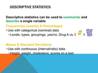
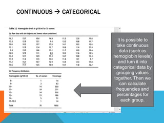
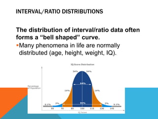
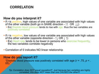
Basic statistics is the science of collecting, organizing, summarizing, and interpreting data. It allows researchers to gain insights from data through graphical or numerical summaries, regardless of the amount of data. Descriptive statistics can be used to describe single variables through frequencies, percentages, means, and standard deviations. Inferential statistics make inferences about phenomena through hypothesis testing, correlations, and predicting relationships between variables.


![HOW DO YOU REPORT T-TESTS RESULTS?
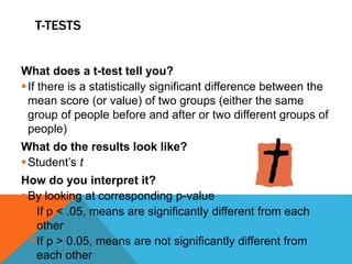
“As can be seen in Figure 1, specialty candidates had
significantly higher scores on questions dealing with treatment
than residency candidates (t = [insert t-value from stats output],
p < .001).
“As can be seen in Figure 1, children’s mean
reading performance was significantly higher on the
post-tests in all four grades, ( t = [insert from stats
output], p < .05)”](https://image.slidesharecdn.com/2teacherspresentation-160331082649/85/statistic-21-320.jpg)