Speech Processing in Stressing Co-Channel Interference Using the Wigner Distribution-Fractional Fourier Transform Algorithm

Seema Sud
Signal Processing: An International Journal (SPIJ), Volume (10) : Issue (1) : 2016 1
Speech Processing in Stressing Co-Channel Interference Using
the Wigner Distribution-Fractional Fourier Transform Algorithm
Seema Sud seema.sud@aero.org
Sr. Engr. Specialist/Communications and Signal Analysis Dept.
The Aerospace Corporation
Chantilly VA, 20191, U.S.A.
Abstract
The Fractional Fourier Transform (FrFT) can provide significant interference suppression (IS)
over other techniques in real-life non-stationary environments because it can operate with very
few samples. However, the optimum rotational parameter ‘a’ must first be estimated. Recently, a
new method to estimate ‘a’ based on the value that minimizes the projection of the product of the
Wigner Distributions (WDs) of the signal-of-interest (SOI) and interference was proposed. This is
more easily calculated by recognizing its equivalency to choosing ‘a’ for which the product of the
energies of the SOI and interference in the FrFT domain is minimized, termed the WD-FrFT
algorithm. The algorithm was shown to estimate ‘a’ more accurately than minimum mean square
error FrFT (MMSE-FrFT) methods and perform far better than MMSE Fast Fourier Transform
(MMSE-FFT) methods, which only operate in the frequency domain. The WD-FrFT algorithm
significantly improves interference suppression (IS) capability, even at low signal-to-noise ratio
(SNR). In this paper, we apply the proposed WD-FrFT technique to recovering a speech signal in
non-stationary co-channel interference. Using mean-square error (MSE) between the SOI and its
estimate as the performance metric, we show that the technique greatly outperforms the
conventional methods, MMSE-FrFT and MMSE-FFT, which fail with just one non-stationary
interferer, and continues to perform well in the presence of severe co-channel interference (CCI)
consisting of multiple, equal power, non-stationary interferers. This method therefore has great
potential for separating co-channel signals in harsh, noisy, non-stationary environments.
Keywords: Co-channel Interference, Fractional Fourier Transform, Minimum Mean-square Error,
Speech, Wigner Distribution.
1. INTRODUCTION
The Fractional Fourier Transform (FrFT) is a very useful method for separating a signal-of-
interest (SOI) from interference and/or noise when the statistics of either are nonstationary [1].
The improvement arises because we utilize fractional time-frequency axes not exploited by
conventional methods based on minimum mean-square error (MMSE) using the Fast Fourier
Transform (FFT), denoted as MMSE-FFT, which operates in the frequency domain only [2]. Time
domain methods have the same limitations as FFT methods, and therefore will not be considered
here. Application of the FrFT requires estimation of the optimum rotational parameter ‘a’, i.e. the
‘ta’ axis. Conventional FrFT methods based on obtaining the MMSE between a desired (training)
signal and its estimate [3], denoted as MMSE-FrFT, fail because they require a large number of
samples in practice [4] and also require stationarity over those samples.
Recently, a method that exploits the relationship that the energy of the FrFT of a signal along an
axis ‘ta’ is the projection of its Wigner Distribution (WD) was proposed [5]. This allows us to
determine the axis where the overlap of the WD of the SOI and interference is minimum. Once
the optimum rotational axis with parameter ‘a’ is obtained, a reduced rank filter eliminates the
interference. This method, termed the WD-FrFT algorithm, is shown to be robust using a binary
phase shift keying (BPSK) signal in non-stationary interference and additive white Gaussian noise
(AWGN), even when the carrier-to-interference ratio (CIR) or signal-to-noise ratio (SNR) is low.

Seema Sud
Here, we study the performance of the WD-FrFT technique for recovering noisy speech signals in
co-channel interference (CCI) and show that even with multiple non-stationary interferers,
performance does not degrade, whereas the conventional MMSE-FrFT and MMSE-FFT methods
fail even with a single interferer. A multiple interferer, non-stationary environment may be found in
cellular systems and in satellite uplinks seeing co-channel interference from cellular systems as
well as other satellite systems. Non-stationarity may arise due to Doppler, frequency drifts,
moving users, etc.
The paper outline is as follows: Section 2 briefly reviews the FrFT and its relation to the WD.
Section 3 describes the adaptive filtering problem, now in the FrFT domain. Section 4 discusses
the WD-FrFT method presented in [5] for estimating the optimum value of ‘a’ and filtering out the
interference and the conventional MMSE-FrFT and MMSE-FFT methods. Section 5 has
simulation results showing the performance of the proposed method with a noisy speech signal
and one or more nonstationary interferers, comparing the WD-FrFT to the conventional methods.
Conclusions and remarks on future work are given in Section 6.
2. FRACTIONAL FOURIER TRANSFORM AND WIGNER DISTRIBUTION
The WD of an SOI and interferer are shown in Fig. 1. In non-stationary environments, both the
SOI x(t) and the interference xI(t) vary as a function of time and frequency. Note that they both
overlap in the time domain (ta=0) and in the frequency domain (ta=1), but there is some axis ta, 0
< a < 2, where they do not overlap, or possibly overlap very little. The WD-FrFT seeks to find this
optimum axis using the FrFT, so we can best filter out the interference [5].
FIGURE 1: Wigner Distribution of Signal x(t) and Interference xI(t) Showing Optimum Axis ta where
Interference May Be Completely Filtered Out.
The WD of a signal x(t) can be written as
(1)
The projection of the WD of a signal x(t) onto an axis ta gives the energy of the signal in the FrFT
domain ‘a’, |Xa(t)|
2
(see e.g. [6] or [7]). Projecting the signal onto domain ‘a’ gives us a measure of
how much of that signal is present in domain ‘a’ similar to what the FFT does using frequency bins.
Letting α = aπ/2, this is written as
(2)

Seema Sud
As the above equation shows, computing signal energy along a particular axis ta with rotational
parameter ‘a’ from the WD is difficult because it requires knowledge of the nature of the signal, and
the ability to rotate it by an angle α and integrate it over the new rotational frequency axis, leaving
the rotational time axis; however, computing |Xα(t)|
2
from the FrFT is a simple and efficient matrix-
vector multiplication ([5], [8], and [9]) that does not require knowledge of the structure of Wx(t,f). In
discrete time, the FrFT of an N × 1 vector x is
(3)
where F
a
is an N × N matrix with elements ([9] and [1])
(4)
and where uk[m] and uk[n] are eigenvectors of the matrix S, defined in [9]. Taking the magnitude
squared of Xa produces the desired result.
3. PROBLEM FORMULATION
Consider a received signal sampled in discrete time, y(i), which we can write as
(5)
where x(i) is a speech signal (the SOI), xI,p(i) are interferers, where p = 1, 2, ..., KI, KI is the total
number of interferers, and n(i) is AWGN. Index i denotes the i
th
sample, where i = 1, 2, ..., N, and N
is the total number of samples per block that we process. We then process M blocks (or trials) to
obtain a statistical estimate of the MMSE. In [5] the SOI was assumed to be a digital binary phase
shift keying (BPSK) signal, whose samples took on the values (+1,−1). Here, we assume x(i) are
samples of a continuous, analog, speech signal. The idea is to perform interference suppression
with samples in the analog domain after digital-to-analog (D/A) conversion of the collected signal at
the receiver. This would allow us to operate on analog samples instead of digitized bits, which
reduces the amount of processing that needs to be done, since digitization typically takes 8 < n <
16 bits per sample. We will show several examples of interferers in Section 5, including another
speech signal, a chirp signal, and a Gaussian pulse with random amplitude and phase, and a
BPSK signal.
We obtain an estimate of the transmitted signal x(i), denoted , by first transforming the received
signal to the FrFT domain, applying an adaptive filter, and taking the inverse FrFT. This is written
as [3]
(6)
where F
a
and F
−a
are the N × N FrFT and inverse FrFT matrices of order ‘a’, respectively, and
(7)
is an N ×1 set of optimum filter coefficients to be found. The notation diag(G) = (g0, g1, ..., gN−1)
means that matrix G has the scalar coefficients g0, g1, ..., and gN−1 as its diagonal elements, with
all other elements equal to zero. Computing the signal estimate therefore requires that we first

Seema Sud
estimate the best rotational parameter ‘a’, and then compute the optimum filter coefficients g0.
This is briefly discussed next.
4. CONVENTIONAL MMSE METHODS AND PROPOSED WD-FRFT METHOD
4.1 Conventional MMSE Methods
MMSE-based methods aim to minimize the error between the desired signal x(i) and its estimate
(i). That is, we minimize the cost function
(8)
It is well known that the optimum set of filter coefficients g0 that minimizes the cost function in Eq.
(8) can be obtained by setting the partial derivative of the cost function to zero [3]. That is,
compute g0 such that
(9)
This is the MMSE-FrFT solution, given by [3]
(10)
where
(11)
(12)
and
(13)
We thus choose the value of ‘a’ as that which minimizes the cost function in Eq. (8). We point out
that we must compute the cost function over the range of ‘a’ from 0 < a < 2 by first computing
g0,MMSE−FrFT from Eq. (10) to find the best value of ‘a’. Note also that this solution requires a
training sequence, x(i). We also mention that the LMS-FrFT solution presented in [10] will perform
comparably to the MMSE-FrFT algorithm over time, hence we do not include it in our simulations.
The MMSE-FFT solution is obtained simply by setting a = 1 in calculating g0 from Eqs. (10)−(13).
This solution simply becomes one of applying the optimum filter given by Eq. (10) in the
frequency domain, since F
1
reduces to an FFT and F
−1
is an inverse FFT (IFFT). In other words,
(14)
4.2 Proposed WD-FrFT Method
The proposed technique estimates the optimum value of ‘a’ while avoiding the pitfalls associated
with the MMSE-FrFT method in [3], namely (1) not relying on the distorted received signal y(i) [5];

Seema Sud
(2) using very few samples, as is required in a non-stationary environment [5]; and (3) avoiding the
computational complexity of matrix inversions [4].
From Fig. 1 and Eq. (2), we can easily compute the WD along each axis ta by computing the
energy of the FrFT along that axis. Hence, the WD-FrFT computes the energy of the FrFT of both
the SOI and interference, computes their product, sums the values over the new time-frequency
axis ta defined by the rotational parameter ‘a’, and selects as the optimum ‘a’ the value for which
the result is minimum [5]. The proposed WD-FrFT algorithm in [5] is repeated here for
convenience:
In this paper, the interference term xI(i) may be composed of multiple interferers such that
(15)
whereas in [5], only one interferer was assumed so KI = 1 and xI(i) represented a single interferer.
Recall that the matrix F
a
was defined in Eq. (4), so to keep it small, we must keep N small. Once
we have the best ‘a’, we compute the filter coefficients g0 in Eq. (7) using the correlations
subtraction architecture of the reduced rank multistage Wiener filter (CSA-MWF) ([11] and [12])
instead of using the MMSE solution in [3]. We initialize the CSA-MWF filter in the conventional
way, except that we rotate to the proper time axis `ta’ by transforming all the variables to the FrFT
domain first. So, using the best value of ‘a’ obtained as described above, we let
(16)
and
(17)
where
(18)
The CSA-MWF computes the D scalar weights wj and vectors hj, j = 1, 2, ..., D from d0(i) and x0(i)
(see Table I for the detailed equations) from which we form the optimum filter
(19)
where D is the filter rank which we typically set to one; this results in a single stage filter which
has the added advantage of fast computation. Note that we need a training sequence x(i) in Step
(2) above, but since N is small, we need just a few samples. Note also that Step (3) above
requires calculation of the FrFT of the interference. Since the algorithm operates with very few

Seema Sud
samples, we can compute this in gaps where the SOI is off, which is common in speech, but this
will include the noise in the channel as well, since we cannot separate that out from the
interference. However, since we collect samples of the environment in the absence of the SOI, it
should not depend on the number of interferers present, as we show later in the next section. In
the following section we compare performance of all three algorithms using a speech signal as
the SOI.
TABLE 1: Recursion Equations for the CSA-MWF.
5. SIMULATIONS
We present simulation examples to compare the MMSE-FrFT and MMSE-FFT methods that
already exist in the literature to the proposed WD-FrFT method for calculating the optimum FrFT
rotational parameter ‘a’. After rotating to the optimum axis ‘ta’, we compute the adaptive filter
coefficients for the three techniques from Eq.’s (10), (14), and (19), respectively. We then use
those coefficients to compute the resultant MSE between the true and estimated SOI by comparing
the signal estimate in Eq. (6) and the true signal x(i). We show that the proposed WD-FrFT
technique provides significantly improved MSE over the existing MMSE-FrFT and MMSE-FFT
methods using one to four interferers, which are at the same power levels as the SOI.
We let the SOI be a speech signal, shown in Fig. 2, obtained by sampling a voice recording for T =
5 seconds at a sampling rate of fs = 6,800 samples per second, giving a total of T·fs = 34,000
samples. This value of T is much larger than the block size N as we will see below. The choice of fs
is typical for a bandlimited speech signal and provides good voice quality. We set the amplitude of
the AWGN based upon a desired SNR [5] and set the amplitude of each interferer to AI,p =
10
−CIRp/20
, where CIRp, p = 1, 2, ..., KI is carrier-to-interference ratio given in dB; note a negative
CIRp means that interferer p is stronger than the SOI. We run the algorithm using M = 1,000 trials,
to obtain histograms of the MSE mean and variance estimates using the three algorithms.
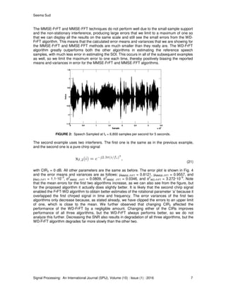
In the first example, we let N = 2 samples per block, and set SNR = 5 dB. We let the interferer be
another speech signal s(i), multiplied by a chirp function, so that
(20)
We set CIR1 = 0 dB, so the interferer is the same strength as the SOI; this is chosen because
equal power signals represent a worst case scenario, i.e. they are the most difficult to separate,
because there is no power difference that can be utilized, so we use 0 dB when we consider other
interferers too. A plot comparing the histograms of the mean-square error of the three techniques
is shown in Fig. 3. If we average over the M = 1,000 trials, we obtain the error means and
variances as follows: µMMSE−FrFT = 0.1171, µMMSE−FFT = 0.3931, and µWD−FrFT = 6.5·10
−3
, σ
2
MMSE−FrFT =
0.0306, σ
2
MMSE−FFT = 0.1442, and σ
2
WD−FrFT = 3.5305·10
−4
. We emphasize that if we make N larger,
MMSE improves slightly, but does worse than WD-FrFT. As we keep increasing N, all three
techniques become worse due to the non-stationarity. Hence, we need to keep N small.

Seema Sud
The MMSE-FrFT and MMSE-FFT techniques do not perform well due to the small sample support
and the non-stationary interference, producing large errors that we limit to a maximum of one so
that we can display all the results on the same scale and still see the small errors from the WD-
FrFT algorithm. This means that the calculated error means and variances that we are showing for
the MMSE-FrFT and MMSE-FFT methods are much smaller than they really are. The WD-FrFT
algorithm greatly outperforms both the other algorithms in estimating the reference speech
samples, with much less error in estimating the SOI. This occurs in all of the subsequent examples
as well, so we limit the maximum error to one each time, thereby positively biasing the reported
means and variances in error for the MMSE-FrFT and MMSE-FFT algorithms.
FIGURE 2: Speech Sampled at fs = 6,800 samples per second for 5 seconds.
The second example uses two interferers. The first one is the same as in the previous example,
and the second one is a pure chirp signal
(21)
with CIR2 = 0 dB. All other parameters are the same as before. The error plot is shown in Fig. 4
and the error means and variances are as follows: µMMSE−FrFT = 0.8121, µMMSE−FFT = 0.9557, and
µWD−FrFT = 1.1·10
−3
, σ
2
MMSE −FrFT = 0.0809, σ
2
MMSE −FFT = 0.0346, and σ
2
WD−FrFT = 3.272·10
−6
. Note
that the mean errors for the first two algorithms increase, as we can also see from the figure, but
for the proposed algorithm it actually does slightly better. It is likely that the second chirp signal
enabled the FrFT-WD algorithm to obtain better estimates of the rotational parameter ‘a’ because it
overlapped the first chirped signal in time and frequency. The error variances of the first two
algorithms only decrease because, as stated already, we have clipped the errors to an upper limit
of one, which is close to the mean. We further observed that changing CIR2 affected the
performance of the WD-FrFT by a negligible amount. Changing either of the CIRs improves
performance of all three algorithms, but the WD-FrFT always performs better, so we do not
analyze this further. Decreasing the SNR also results in degradation of all three algorithms, but the
WD-FrFT algorithm degrades far more slowly than the other two.

Seema Sud
FIGURE 3: MSE Comparison with Single Chirped Speech Interferer; CIR1 = 0 dB, SNR = 5 dB, N = 2.
FIGURE 4: MSE Comparison with Chirped Speech and Chirped Signal Interferers; CIR1 = CIR2 = 0 dB,
SNR = 5 dB, N = 2.

Seema Sud
In the next example, we add a third interferer in the form of a Gaussian pulse, given by
(22)
where β and ϕ are the amplitude and phase of the pulse, respectively, uniformly distributed in
(1,1.5), again using the worst case of CIR3 = 0 dB. All other parameters are the same as before.
The error plot is shown in Fig. 5 and the error means and variances are as follows: µMMSE−FrFT =
0.8044, µMMSE−FFT = 0.9491, and µWD−FrFT = 1.2·10
−3
, σ
2
MMSE−FrFT = 0.0888, σ
2
MMSE−FFT = 0.0368, and
σ
2
WD−FrFT = 9.690·10
−6
. Note that the mean errors for the first two algorithms increase, but the
proposed algorithm still does nearly as well as the previous case. The error variances for the first
two algorithms increase only slightly, so we have a larger overall error but not a spread in errors.
This could of course also be affected by our limiting of the errors, because we observe a small
percentage of very large errors if we do not limit them. The error variance of the proposed
technique increases but is still orders of magnitude smaller than for the other two methods.
In the final example, we include a fourth interferer in the form of a BPSK signal, where the bits b(i)
are randomly chosen in (+1,−1) and again CIR4 = 0 dB. We add a small frequency offset to the
baseband signal,
(23)
FIGURE 5: MSE Comparison with Chirped Speech, Chirp Signal, and Gaussian Pulse Interferers; CIR1 =
CIR2 = CIR3 = 0 dB, SNR = 5 dB, N = 2.
All other parameters are again the same as before. The error plot is shown in Fig. 6 and the error
means and variances are as follows: µMMSE−FrFT = 0.4471, µMMSE−FFT = 0.7218, and µWD−FrFT =
0.0239, σ
2
MMSE−FrFT = 0.1813, σ
2
MMSE−FFT = 0.143, andσ
2
WD−FrFT = 2.1·10
−3
. Note that the mean
errors for the first two algorithms decrease slightly but the variance is now higher, indicating

Seema Sud
greater spread and larger errors. In this case, we finally see a degradation in performance of the
proposed WD-FrFT algorithm. This is because the BPSK signal overlaps with the SOI significantly
in the WD domain, reducing the ability of the algorithm to separate them. However, it still performs
very well. Our results indicate that the WD-FrFT can perform reliable IS with an arbitrary number
of interferers. The algorithm degrades only when an interferer begins to overlap the SOI in the
WD plane, but the degradation is graceful and errors are still small.
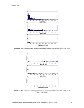
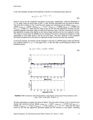
FIGURE 6: MSE Comparison with Chirped Speech, Chirp Signal, Gaussian Pulse, and BPSK Interferers;
CIR1 = CIR2 = CIR3 = CIR4 = 0 dB, SNR = 5 dB, N = 2.
6. CONCLUSION
In this paper, we study the WD-FrFT algorithm for suppressing multiple non-stationary interferers
in processing and recovering speech. The algorithm is robust in low sample support, low carrier-
to-interference ratio (CIR), and low signal to noise ratio (SNR) where conventional MMSE-FrFT
and MMSE-FFT techniques fail. We show that the method continues to perform well with multiple
non-stationary interferers. Use of this technique could greatly enhance the ability to demodulate
signals in high interference environments, and if a rotational axis can be found where the
interference does not overlap the SOI, perfect interference cancellation may be done. Future
work includes applying the WD-FrFT algorithm to over-the-air real-world signals, and applying it
to other fields such as geolocation and radar.
7. ACKNOWLEDGMENTS
The author thanks The Aerospace Corporation for funding this work, Alan Foonberg for reviewing
the paper, and the anonymous reviewers for comments that improved the quality of the paper.
8. REFERENCES
[1] H.M. Ozaktas, Z. Zalevsky, and M.A. Kutay, “The Fractional Fourier Transform with
Applications in Optics and Signal Processing”, West Sussex, England: John Wiley and Sons,
2001.

Seema Sud
[2] L.B. Almeida, “The Fractional Fourier Transform and Time-Frequency Representation”, IEEE
Trans. on Sig. Proc., Vol. 42, No. 11, pp. 3084-3091, Nov. 1994.
[3] S. Subramaniam, B.W. Ling, and A. Georgakis, “Filtering in Rotated Time-Frequency
Domains with Unknown Noise Statistics”, IEEE Trans. on Sig. Proc., Vol. 60, No. 1, pp. 489-
493, Jan. 2012.
[4] I.S. Reed, J.D. Mallett, and L.E. Brennan, “Rapid Convergence Rate in Adaptive Arrays”,
IEEE Trans. on Aerospace and Electronic Systems, Vol. 10, pp. 853-863, Nov. 1974.
[5] S. Sud, “Estimation of the Optimum Rotational Parameter of the Fractional Fourier Transform
Using its Relation to the Wigner Distribution”, International Journal of Emerging Technology
and Advanced Engineering (IJETAE), Vol. 5, No. 9, pp. 77-85, Sep. 2015.
[6] M.A. Kutay, H.M. Ozaktas, O. Arikan, and L. Onural, “Optimal Filtering in Fractional Fourier
Domains”, IEEE Trans. on Sig. Proc., Vol. 45, No. 5, pp., May 1997.
[7] M.A. Kutay, H.M. Ozaktas, L. Onural, and O. Arikan, “Optimal Filtering in Fractional Fourier
Domains”, Proc. IEEE Int. Conf. on Acoustics, Speech, and Sig. Proc. (ICASSP), Vol. 2, pp.
937-940, May 9-12, 1995.
[8] C. Candan, M.A. Kutay, and H.M. Ozaktas, “The Discrete Fractional Fourier Transform”, Proc
Int. Conf. on Acoustics, Speech, and Sig. Proc. (ICASSP), Phoenix, AZ, pp. 1713-1716, Mar.
15-19, 1999.
[9] C. Candan, M.A. Kutay, and H.M. Ozaktas, “The Discrete Fractional Fourier Transform”,
IEEE Trans. on Sig. Proc., Vol. 48, pp. 1329-1337, May 2000.
[10] Q. Lin, Z. Yanhong, T. Ran, and W. Yue, “Adaptive Filtering in Fractional Fourier Domain”,
International Symposium on Microwave, Antenna, Propagation, and EMC Technologies for
Wireless Communications Proc., pp. 1033-1036.
[11]J.S. Goldstein and I.S. Reed, “Multidimensional Wiener Filtering Using a Nested Chain of
Orthogonal Scalar Wiener Filters”, University of Southern California, CSI-96-12-04, pp. 1-7,
Dec. 1996.
[12]D.C. Ricks, and J.S. Goldstein, “Efficient Architectures for Implementing Adaptive
Algorithms”, Proc. of the 2000 Antenna Applications Symposium, Allerton Park, Monticello,
Illinois, pp. 29-41, Sep. 20-22, 2000.

Speech Processing in Stressing Co-Channel Interference Using the Wigner Distribution-Fractional Fourier Transform Algorithm

More Related Content

What's hot

Similar to Speech Processing in Stressing Co-Channel Interference Using the Wigner Distribution-Fractional Fourier Transform Algorithm

Recently uploaded

Speech Processing in Stressing Co-Channel Interference Using the Wigner Distribution-Fractional Fourier Transform Algorithm