Download as PDF, PPTX

![Introduction Sparse FHT algorithm Analysis of probability of failure Empirical results Conclusion
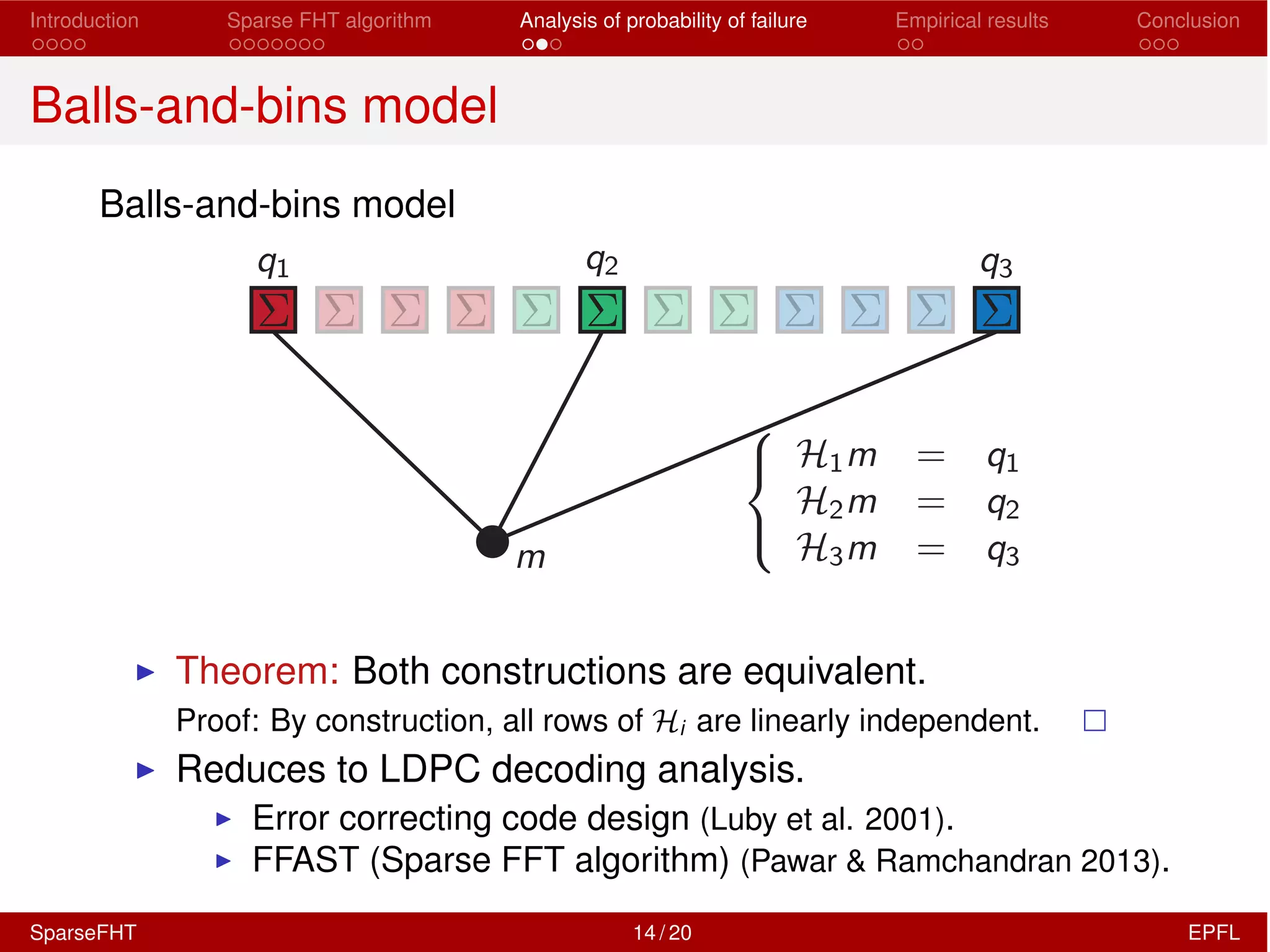
SparseFHT vs. FHT
Runtime [µs] – N = 215
0 1/3 2/3 1
0
200
400
600
800
1000
Sparse FHT
FHT
↵
SparseFHT 17 / 20 EPFL](https://image.slidesharecdn.com/sparsefht-150529123958-lva1-app6891/75/A-Fast-Hadamard-Transform-for-Signals-with-Sub-linear-Sparsity-79-2048.jpg)

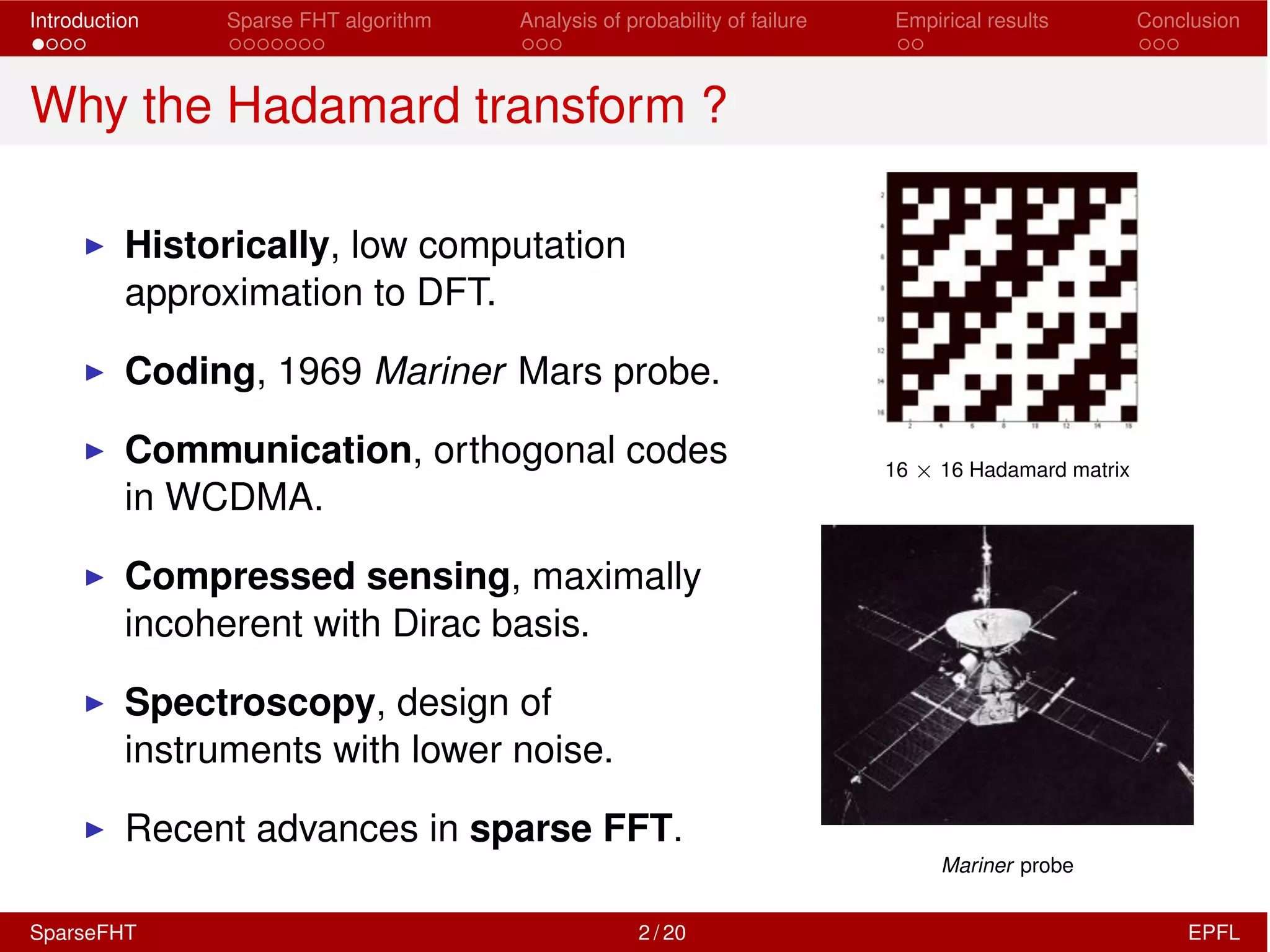
![Introduction Sparse FHT algorithm Analysis of probability of failure Empirical results Conclusion
Reference
[1] M.G. Luby, M. Mitzenmacher, M.A. Shokrollahi, and
D.A. Spielman,
Efficient erasure correcting codes,
IEEE Trans. Inform. Theory, vol. 47, no. 2,
pp. 569–584, 2001.
[2] S. Pawar and K. Ramchandran,
Computing a k-sparse n-length discrete Fourier transform
using at most 4k samples and O(k log k) complexity,
arXiv.org, vol. cs.DS. 04-May-2013.
SparseFHT 20 / 20 EPFL](https://image.slidesharecdn.com/sparsefht-150529123958-lva1-app6891/75/A-Fast-Hadamard-Transform-for-Signals-with-Sub-linear-Sparsity-83-2048.jpg)

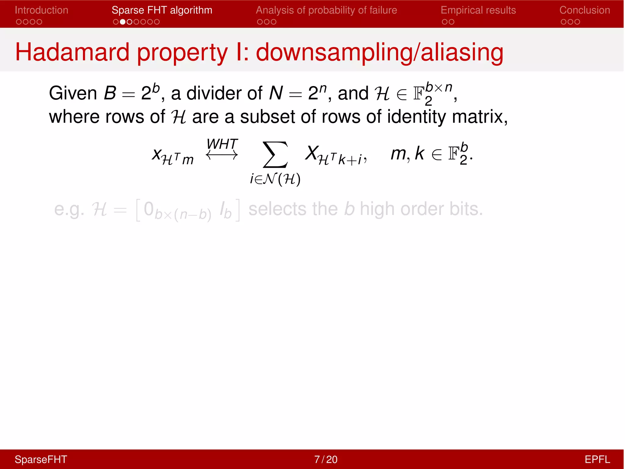
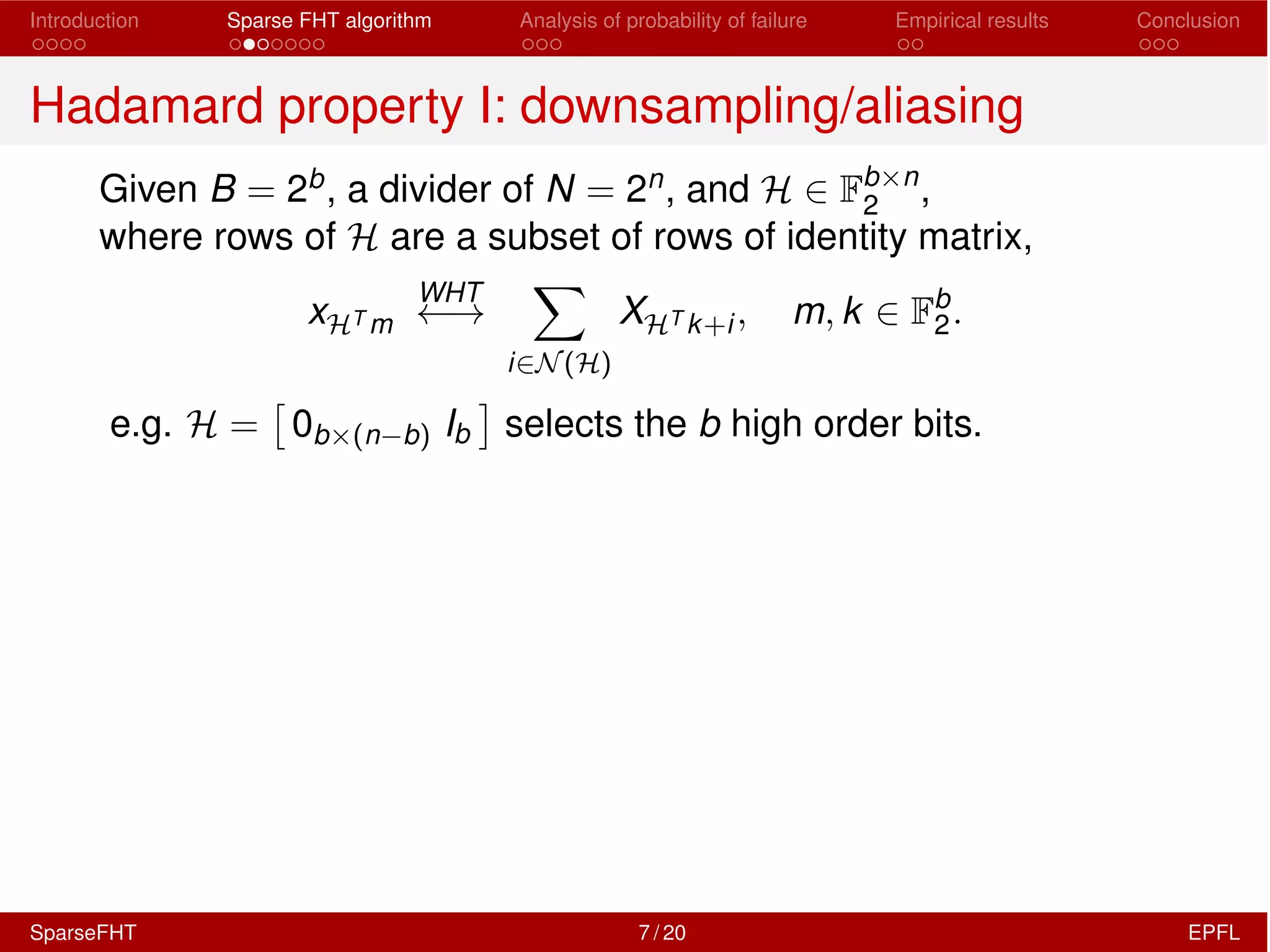
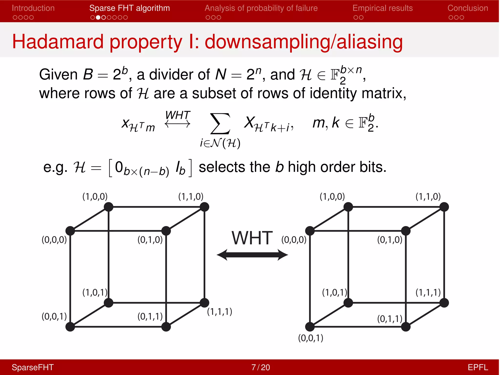
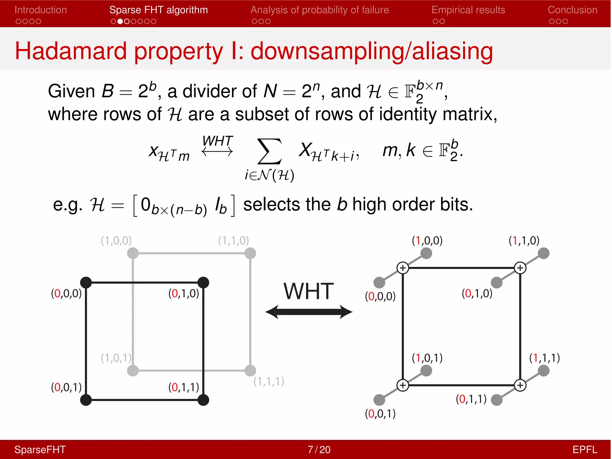
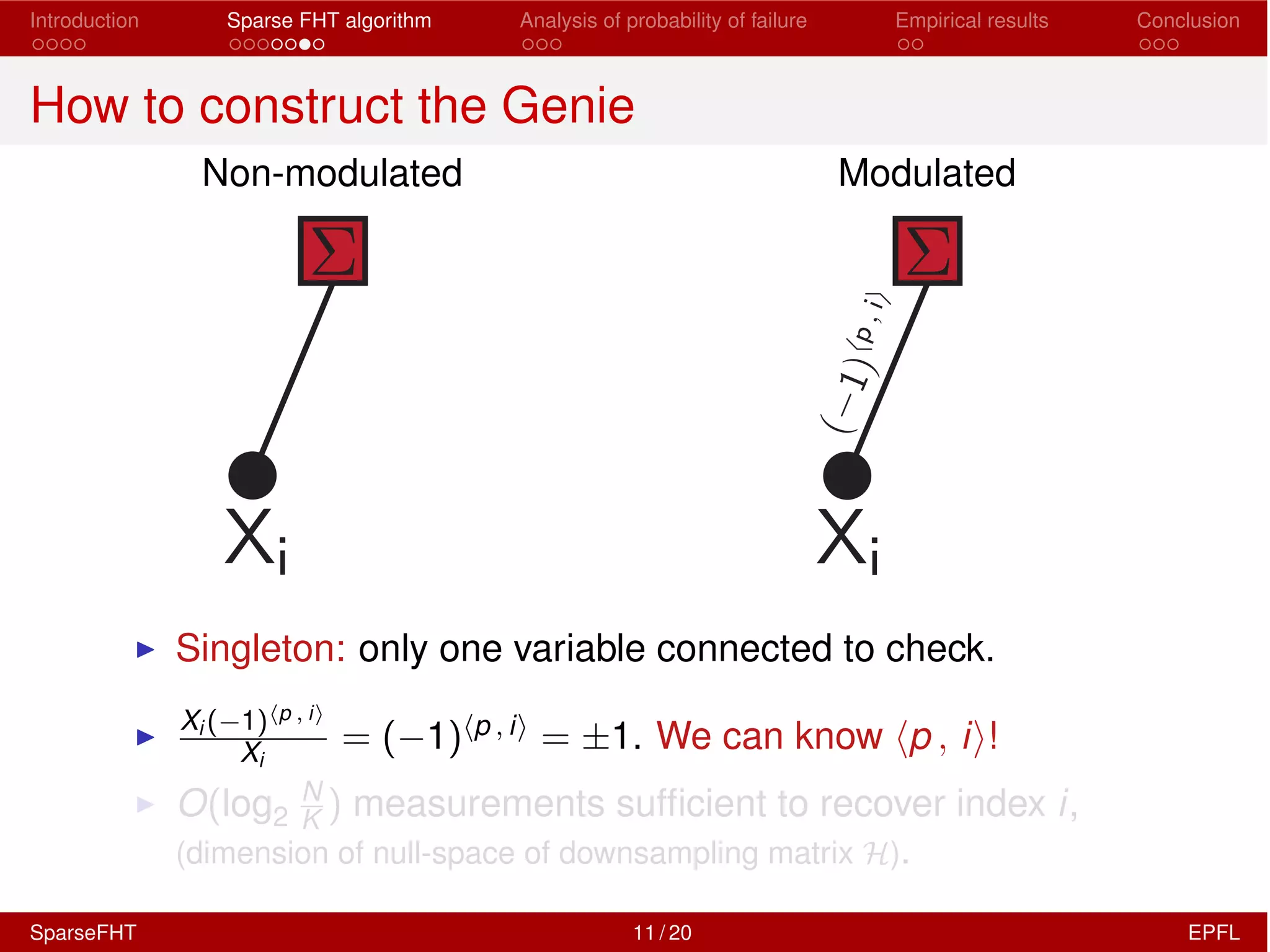
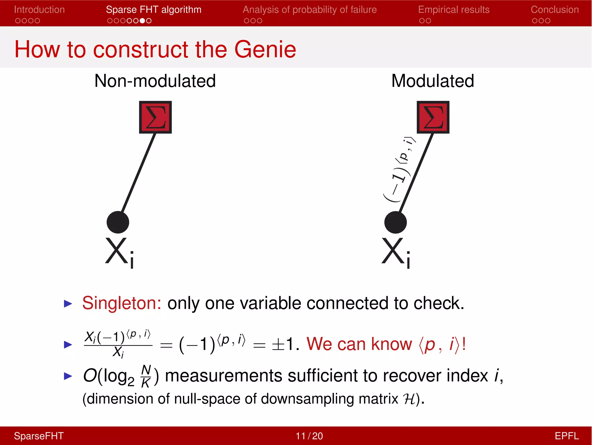
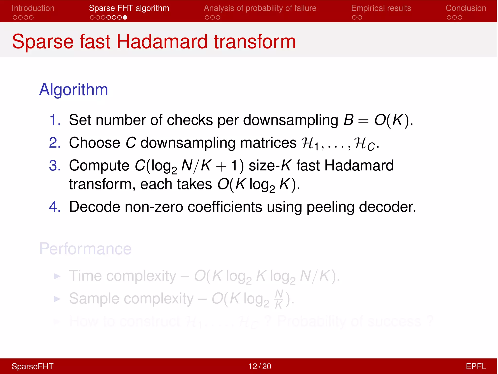
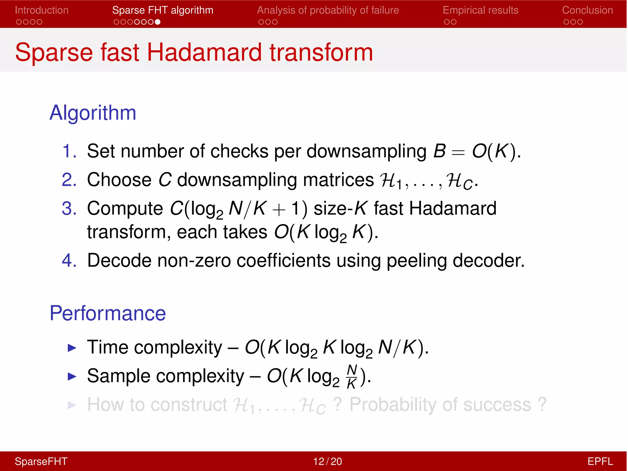
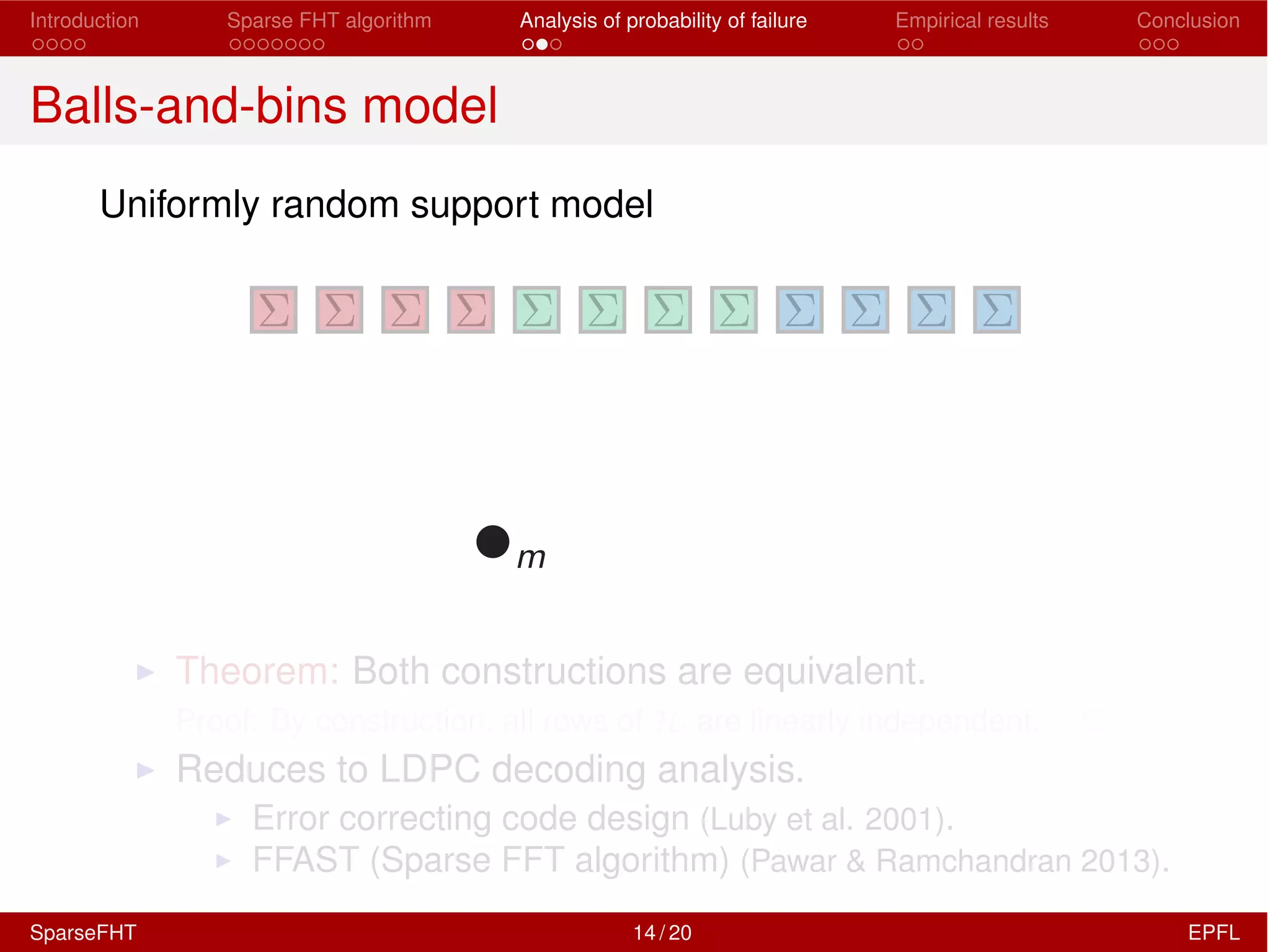
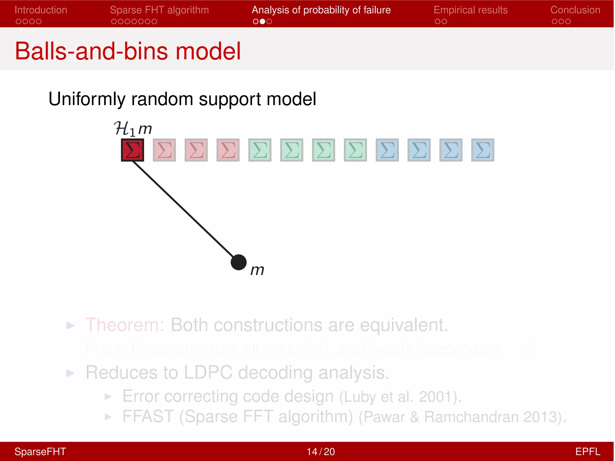
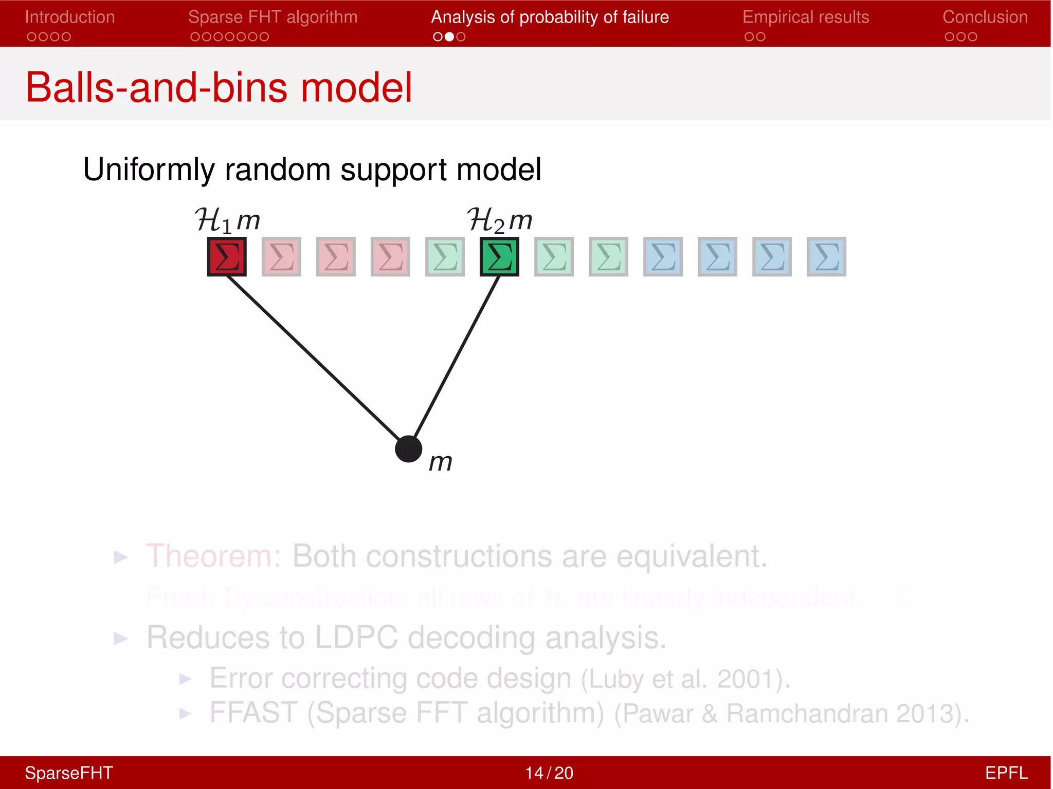
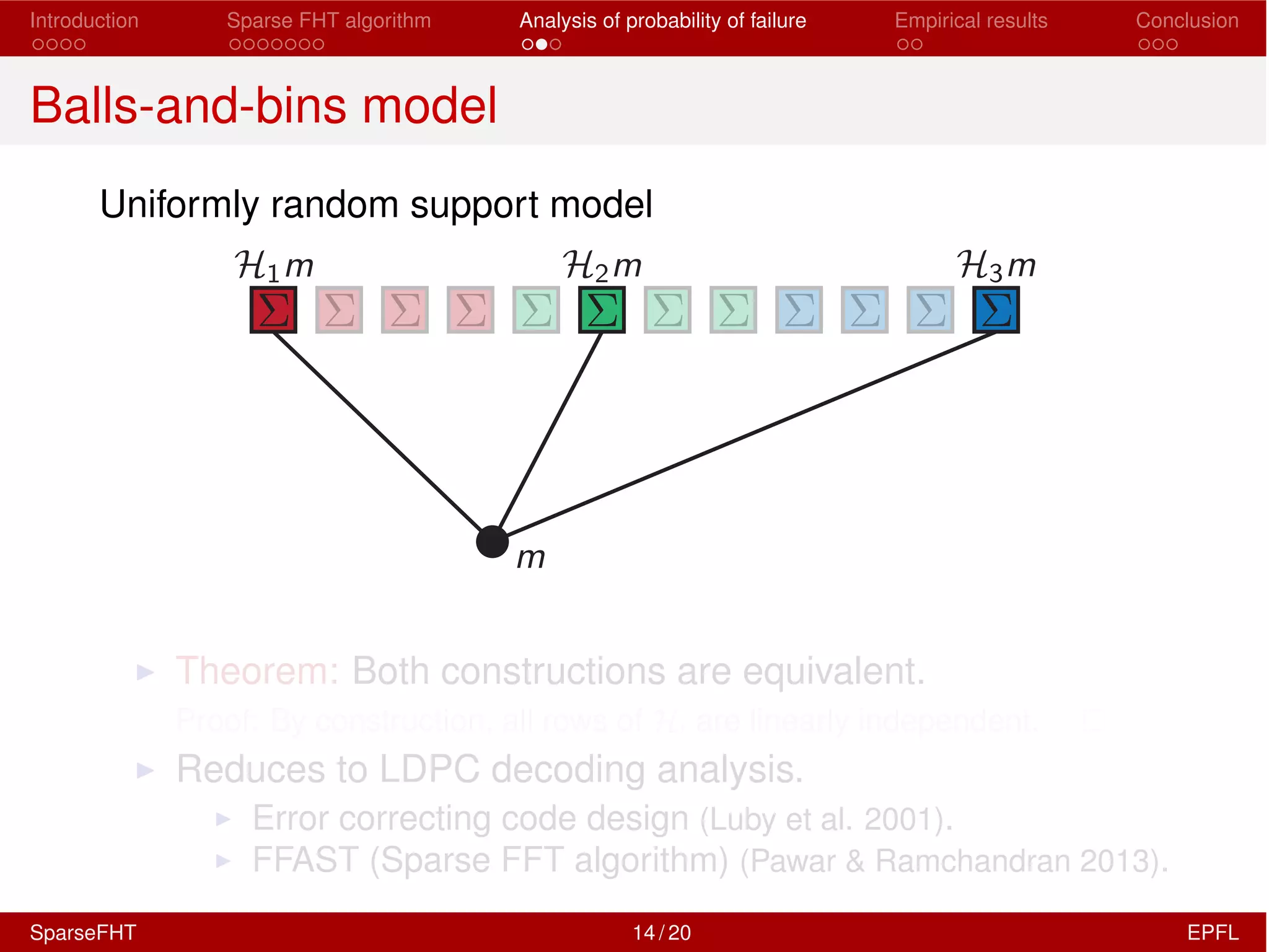
The document discusses the development of a Sparse Fast Hadamard Transform (Sparse FHT) algorithm which efficiently computes the non-zero coefficients of k-sparse signals in a universal setting. It highlights the algorithm's improvements over traditional Hadamard transforms, achieving faster computation times and reduced sample complexity. Empirical results and analyses of failure probabilities reinforce the efficacy of this new algorithm.