Download as PDF, PPTX

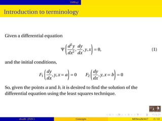
![Least squares method
Formulation II
Least squares method
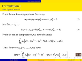
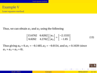
For the least squares issue, we have to compute
F =
b
a
[ (x)]2
dx =
b
a
n
i=0
αi i(i−1)xi−2
+ixi−1
P(xj)+xi
Q(x) −R(x)
2
dx
Therefore,
∂F
∂αi
=
b
a
n
i=0
αi i(i−1)xi−2
+ixi−1
P(x)+xi
Q(x) −R(x) ×
i(i−1)xi−2
+ixi−1
P(x)+xi
Q(x) dx = 0
This, and the equations generated by the boundary conditions can be
solved by using Linear Algebra.
shudh (JNEC) Concepts MEStru2k1617 6 / 12](https://image.slidesharecdn.com/leastsquaremethod-170117150733/85/Solve-ODE-BVP-through-the-Least-Squares-Method-6-320.jpg)
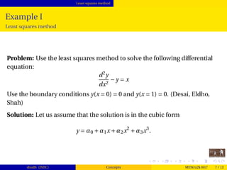

The document discusses solving ordinary differential equations (ODEs) using the least squares finite element method, focusing on minimizing the sum of squares to find solutions. It provides examples of boundary value problems, formulates the least squares method, and demonstrates its application through step-by-step calculations. The content is primarily aimed at civil engineering applications and includes numerical examples to elucidate the method.