Download to read offline


![26
experiment type, expression similarity), they may incorporate these inputs in
different ways. For instance, both SHARAN and DENG use “experiment
type” as input, but SHARAN explicitly includes each type of experiment as a
separate indicator variable in its logistic regression function, while DENG
pools data from each experimental type and assigns a single confidence level
to the interactions in each pool.
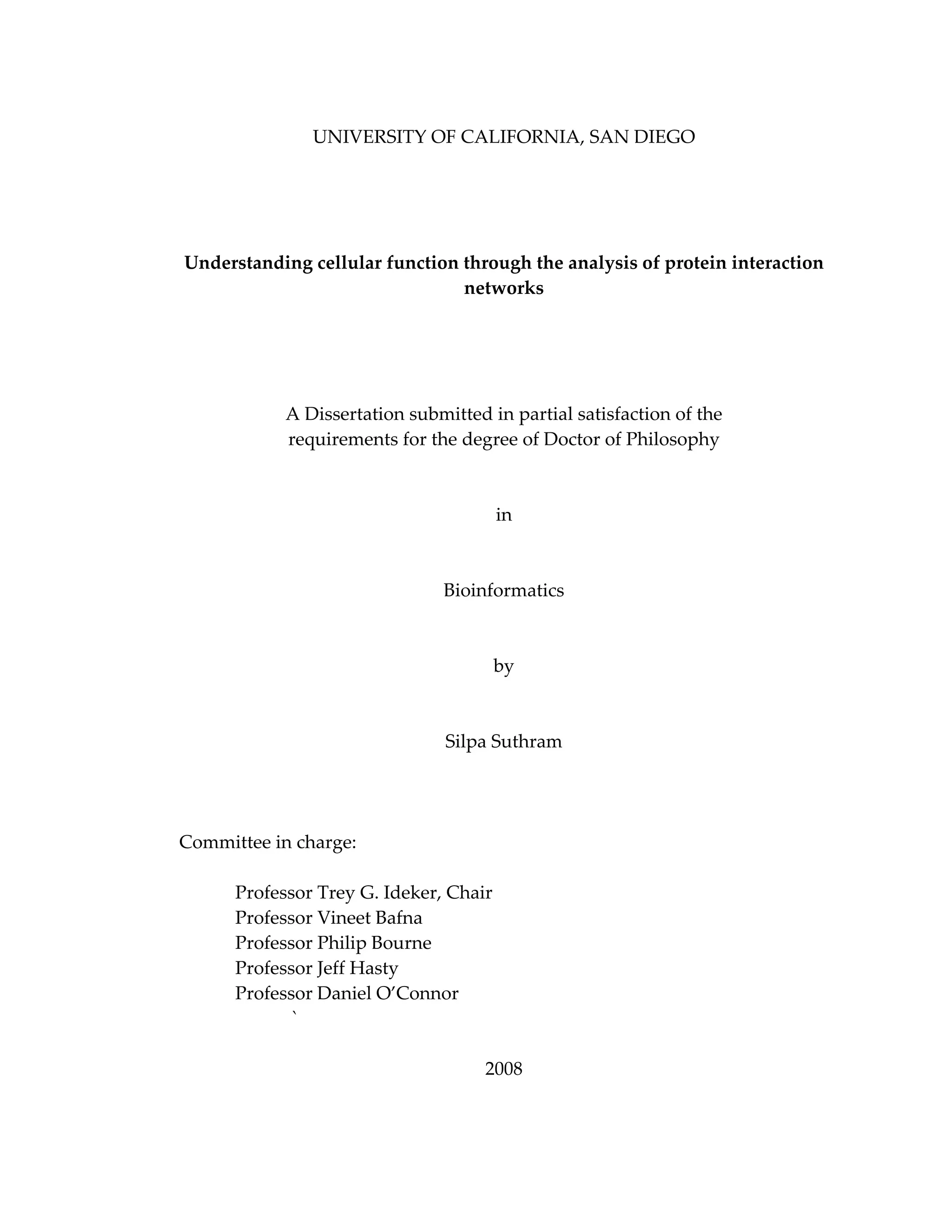
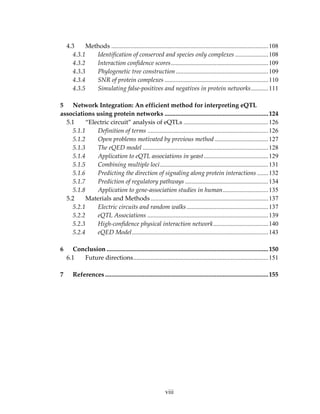
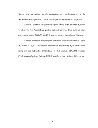
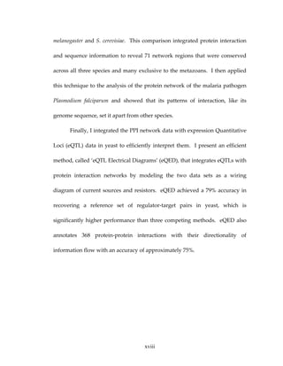
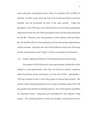
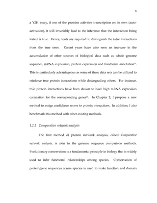
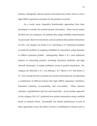
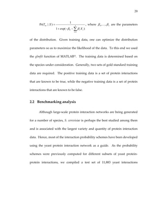
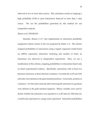
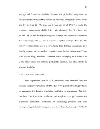
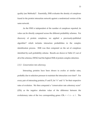
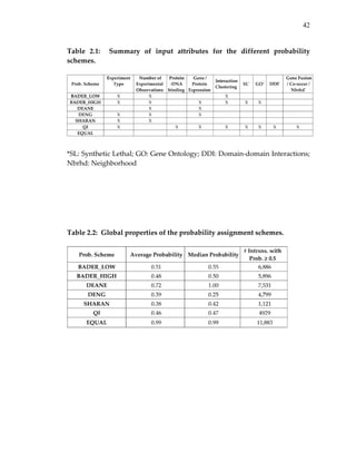
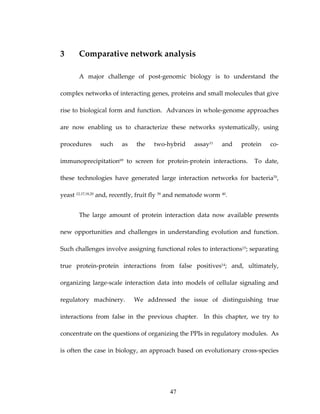
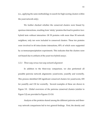
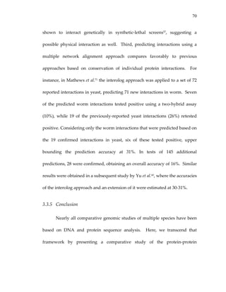
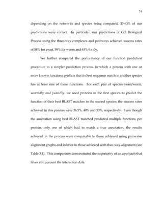
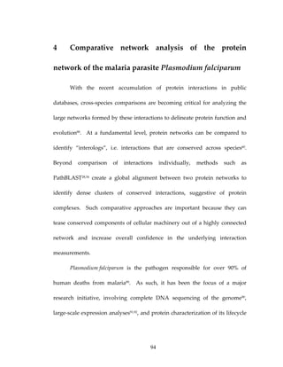
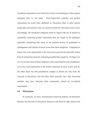
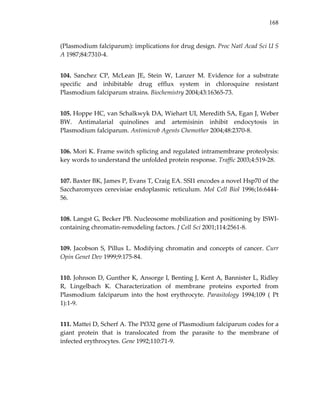
We also compared global statistics such as the average and median
probability assigned by each scheme (see Table 2.2). We found that most
probability schemes had an average probability in the range of [0.3 ‐ 0.5]. In
contrast, Deane et al. (DEANE) had a very high average and median
probability: over half of the interactions in the test set were assigned a
probability of 1. We also computed Spearman correlations among the different
probability schemes to measure their levels of inter‐dependency (Table 2.3).
The maximum correlation was seen between BADER_LOW and
BADER_HIGH, as might be expected since both schemes were reported in the
same study and BADER_HIGH was derived from BADER_LOW. On the
other hand, Qi et al. (QI) had very low Spearman correlation with any of the
probability schemes. The low correlation may reflect an inherent difference
between schemes that assign probabilities to experimentally observed](https://image.slidesharecdn.com/0585808f-97e2-4cab-9576-ce24b5c02f6d-150410123344-conversion-gate01/85/SilpaSuthram-Thesis-44-320.jpg)

![46
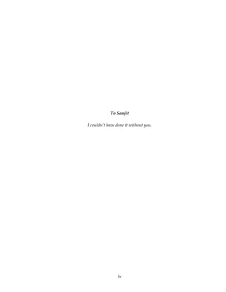
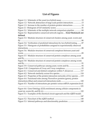
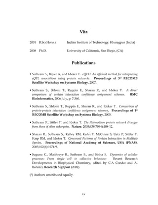
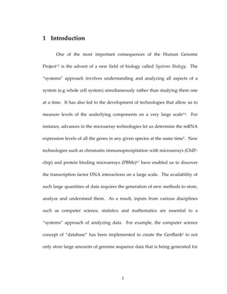
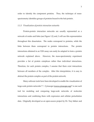
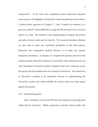
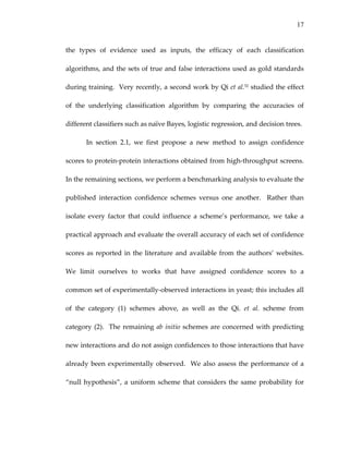
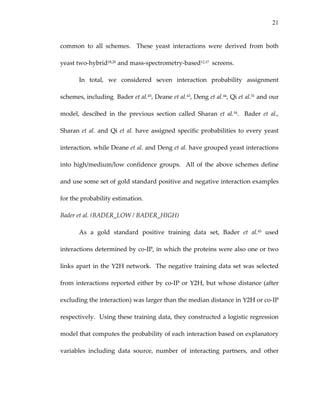
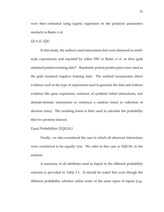
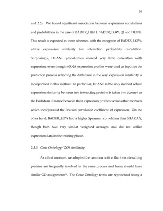
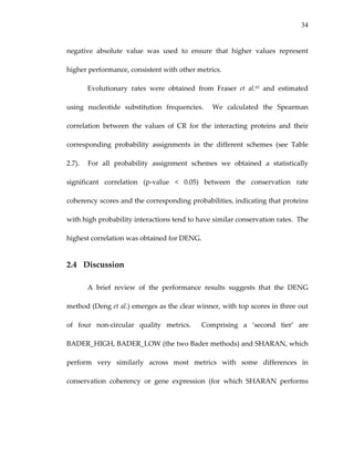
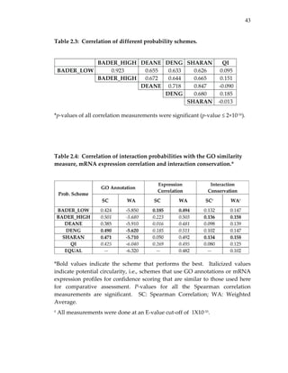
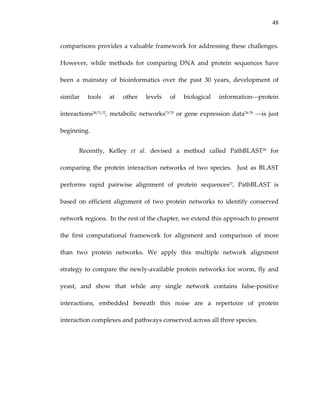
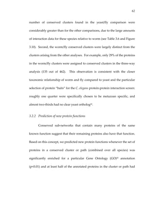
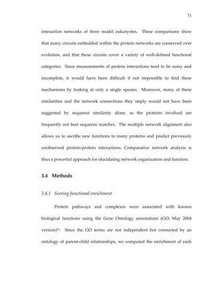
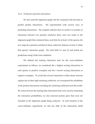
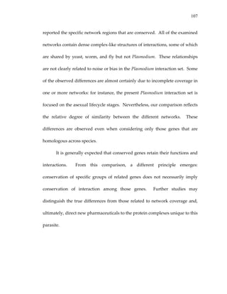
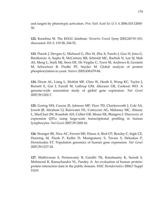
Table 2.7: Associations of conservation rate coherency scores and SNR with
interaction probabilities.
* SC: Spearman Correlation. Bold values indicate the scheme which performs
the best. Note that conservation scores based on weighted averages were
omitted as they were very similar across the different confidence assignment
schemes.
Table 2.8: Fractional scores of the confidence assignment schemes in each
of the five quality measures.*
*Fractional scores are between [0,1] with 1 performing the best (indicated in
bold for each measure). Cells with a dash (‐) indicate circularity, i.e., the
measures used as (full or partial) input to the corresponding probability
schemes. SC: Spearman Correlation; SNR: Signal to Noise Ratio.](https://image.slidesharecdn.com/0585808f-97e2-4cab-9576-ce24b5c02f6d-150410123344-conversion-gate01/85/SilpaSuthram-Thesis-64-320.jpg)
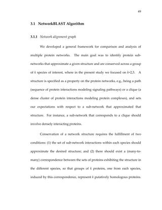
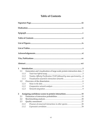
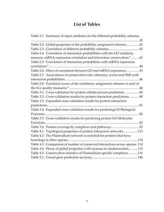
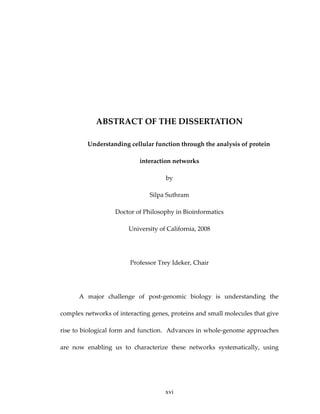
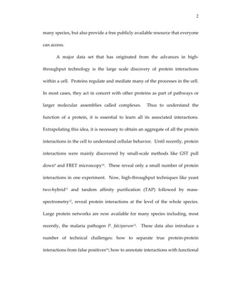
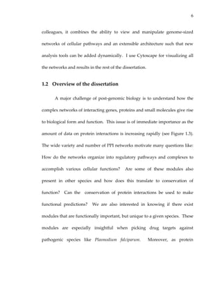
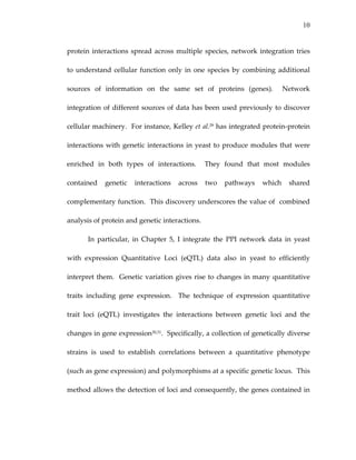
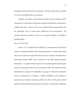
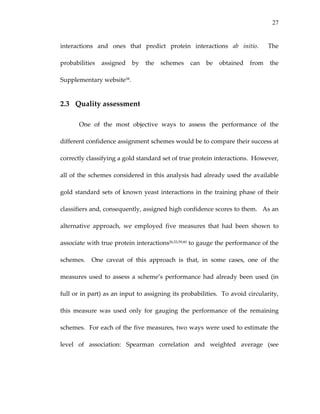
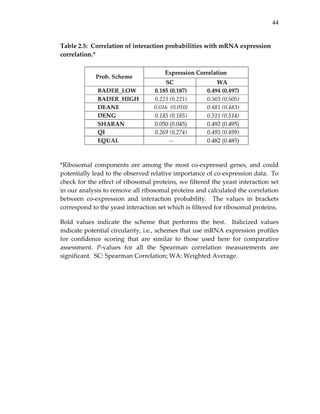
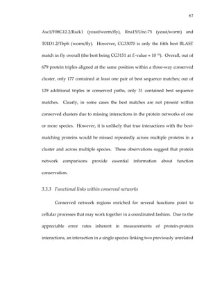
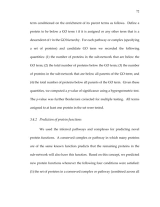
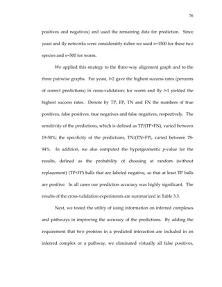
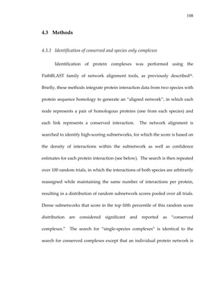
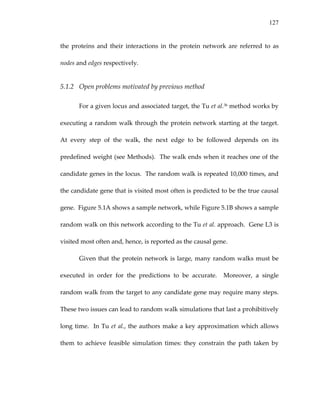
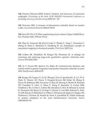
![53
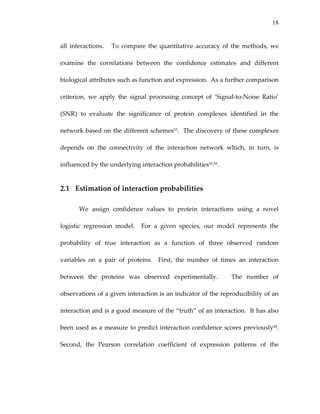
nodes with higher degrees have higher probability. We estimate these
probabilities using a Mote‐Carlo approach as described in Sharan et al.72
Next, we refine the above models to the realistic case in which we are
give partial, noisy observations of the true interaction data. In this case, the
probabilistic model must distinguish between observed interactions and true
interactions. For ease of presentation we concentrate on the case that the
target structure is a clique (corresponding to a protein complex), but the
models generalizes to other structures as well. Let us denote by Tuv the event
that two proteins u,v interact, and by Fuv the event that they do not interact.
Denote by Ouv the (possibly empty) set of available observations on the
proteins u and v, that is, the set of experiments in which an interaction
between u and v was or was not observed. Given a subset U of the nodes, we
wish to compute the likelihood of U under a sub‐network model and under a
null model. Denote by Ou the collection of all observations on node pairs in U.
Under the assumption that all pairwise interactions are independent we have:
( ) ( )
( ) ( ) ( ) ([ ]
( ) ( )[ ]∏
∏
∏
×∈
×∈
×∈
−+=
+=
=
UUvu
uvuvuvuv
UUvu
suvsuvuvsuvsuvuv
UUvu
suvsU
FOTO
MFMFOMTMTO
MOMO
),(
),(
),(
|Pr)1(|Pr
|Pr,|Pr|Pr,|Pr
|Pr|Pr(
ββ
)](https://image.slidesharecdn.com/0585808f-97e2-4cab-9576-ce24b5c02f6d-150410123344-conversion-gate01/85/SilpaSuthram-Thesis-71-320.jpg)
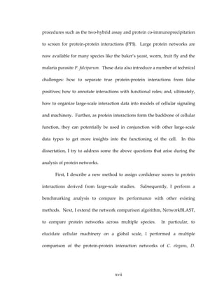
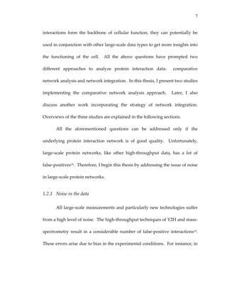
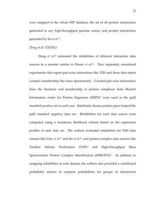
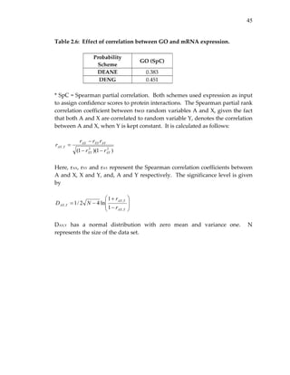
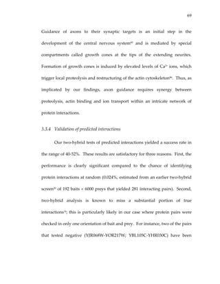
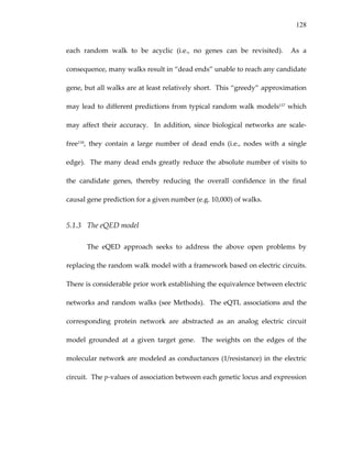
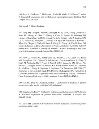
![54
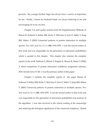
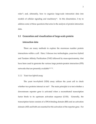
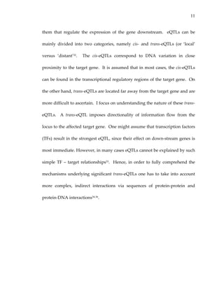
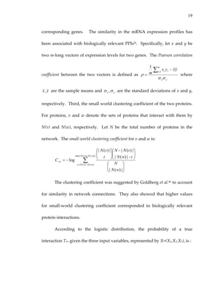
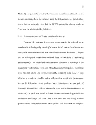
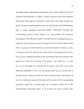
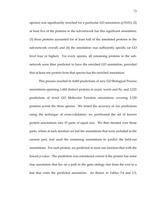
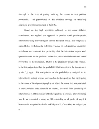
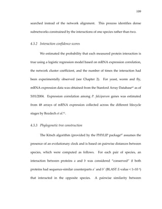
To compute Pr(Ou|Mn) we must update the null model, which depends
on knowing the degree sequence of the interaction graph. We overcome this
difficulty by approximating the degree of each node I in the hidden interaction
graph by its expected degree, di. This refined model assumes that G is drawn
uniformly at random from the collection of all graphs whose degree sequence
is . This induces a probability puv for every node pair (u,v). Thus, we
have:
ndd K,1
( ) ( )[ ] ( )∏×∈
−+=
UUvu
uvuvuvuvuvuvnU FOpTOpMO
),(
|Pr)1(|Pr|Pr
Finally, the log‐likelihood ratio that we assign to a subset of nodes U is
( )
( )
( )
( ) (
( ) (
)
)∑×∈ −+
−+
==
UUvu uvuvuvuvuvuv
uvuvuvuv
nU
sU
FOpTOp
FOTO
MO
MO
UL
),( |Pr)1(|Pr
|Pr)1(|Pr
log
|Pr
|Pr
log
ββ
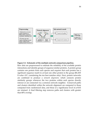
3.1.3 Search algorithm
Using the above model, the problem of identifying conserved protein
networks reduces to the problem of identifying high‐scoring subgraphs of the
network alignment graph. This problem is computationally hard72. Thus, we
present a heuristic strategy for the search problem.
We perform a bottom‐up search for high‐scoring subgraphs in the
alignment graph. The highest scoring paths with four nodes are identified](https://image.slidesharecdn.com/0585808f-97e2-4cab-9576-ce24b5c02f6d-150410123344-conversion-gate01/85/SilpaSuthram-Thesis-72-320.jpg)
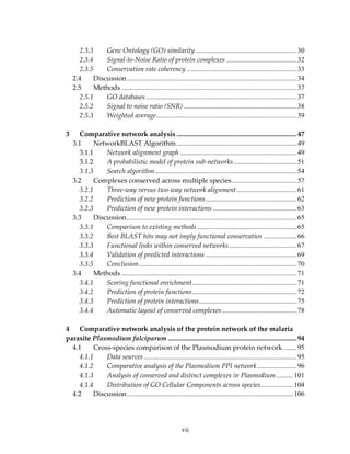
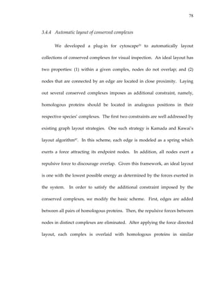
![63
that annotation. When these criteria were met, all remaining proteins in the
sub‐network were predicted to have the enriched GO annotation (see
Methods).
This process resulted in 4,669 predictions of new GO Biological Process
annotations spanning 1,442 distinct proteins in yeast, worm and fly; and 3,221
predictions of novel GO Molecular Function annotations spanning 1,120
proteins. We estimated the specificity of these predictions using the technique
of cross validation, in which one hides part of the data, uses the rest of the
data for prediction, and tests the prediction success using the held‐out data
(see Methods). As shown in Table 3.1, depending on the species, 58‐63% of
our predictions of GO Processes agreed with the known annotations (see also
Tables 3.3 and 3.4). This analysis outperformed a sequence‐based method of
annotating proteins based on the known functions of their best sequence
matches, for which the accuracy ranged between 37 and 53% (see Methods).
3.2.3 Prediction of new protein interactions
We also used the multiple network alignment to predict new protein‐
protein physical interactions. We predicted an interaction between a pair of
proteins based on [1] evidence that proteins with similar sequences interact](https://image.slidesharecdn.com/0585808f-97e2-4cab-9576-ce24b5c02f6d-150410123344-conversion-gate01/85/SilpaSuthram-Thesis-81-320.jpg)
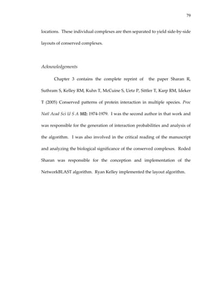
![64
within other species (directly, or via a common network neighbor) and,
optionally, [2] co‐occurrence of these proteins in the same conserved cluster or
path. The accuracy of these predictions was evaluated using five‐fold cross
validation, as described in the Methods section. In cross validation, strategy
[1] achieved 77‐84% specificity and 23‐50% sensitivity, depending on the
species for which the predictions were made (see Table 3.2 and 3.5). These
results were highly significant for the three species. Combining both
strategies [1] and [2] resulted in eliminating virtually all false positive
predictions (specificity>99%), while greatly reducing the number of true
positives, yielding sensitivities of 10% and lower (see Table 3.2). Given the
elevated specificity of the combined strategies, we were able to predict 176
new interactions for yeast, 1,139 for worm and 1,294 for fly with high
confidence. Thus, although protein interactions have been used previously to
predict interactions among the orthologous proteins of other species40,60,
screening these against conserved paths and clusters markedly improves the
specificity of prediction. The complete list of predicted protein interactions is
provided on our website.
To further evaluate the utility of protein interaction prediction based on
network conservation, we tested experimentally 65 of the interactions that](https://image.slidesharecdn.com/0585808f-97e2-4cab-9576-ce24b5c02f6d-150410123344-conversion-gate01/85/SilpaSuthram-Thesis-82-320.jpg)
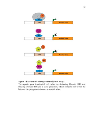
![65
were predicted for yeast using the combined strategies [1] and [2] above
(Figure 3.4a). The tests were performed using two‐hybrid assays11,20, which
are based on a reporter gene that is transcriptionally activated if the two tested
proteins (bait and prey) can physically interact (see Methods and Figure 3.4b).
Five of the tests involved baits that induced reporter activity in the absence of
any prey (Figure 3.4c). Of the remaining 60 putative interactions, 31 tested
positive (more conservatively, 19 out of 48—see Figure 3.4) yielding an overall
success rate in the range of 40‐52%.
3.3 Discussion
3.3.1 Comparison to existing methods
Kelley et al.28 previously developed pairwise network alignment
algorithms that were used to detect linear paths and Sharan et al.72 found
dense clusters that are conserved between yeast and the bacteria H. pylori. The
multiple network alignment scheme that we have presented here is an
extension of these earlier approaches to handle more than two species.
Additional advantages of the current approach over the previous ones are: [1]
a unified method to detect both paths and clusters, which generalizes to other
network structures; [2] incorporation of a refined probabilistic model for](https://image.slidesharecdn.com/0585808f-97e2-4cab-9576-ce24b5c02f6d-150410123344-conversion-gate01/85/SilpaSuthram-Thesis-83-320.jpg)
![66
protein interaction data; and [3] an automatic system for laying out and
visualizing the resulting conserved sub‐networks. A related method that uses
cross‐species data for predicting protein interactions is the interolog
approach71,78: a pair of proteins in one species is predicted to interact if their
best sequence matches in another species were reported to interact. In
comparison, our proposed scheme can associate proteins that are not
necessarily each other’s best sequence match. This confers increased flexibility
in detecting conserved function by allowing for paralogous family expansion
and contraction, or gene loss. Since conservation is evaluated in the context of
a protein interaction sub‐network and not independently for each interaction,
the high specificity of the resulting predictions can be maintained (see below
section “Validation of predicted interactions”).
3.3.2 Best BLAST hits may not imply functional conservation
Frequently, the network alignment associates sequence‐similar proteins
between species even though they are not each other’s best sequence match.
For instance, the conserved network region in Figure 3.2[h] suggests that the
worm protein exc‐7 plays the same functional role as yeast Pab1 and fly
CG33070 (BLAST E‐value ≈ 10 42) based on the conserved interactions with](https://image.slidesharecdn.com/0585808f-97e2-4cab-9576-ce24b5c02f6d-150410123344-conversion-gate01/85/SilpaSuthram-Thesis-84-320.jpg)
![68
processes would typically be ignored as a false positive. However, an
observation that two or three networks reinforce this interaction is
considerably more compelling, especially when the interaction is embedded in
a densely‐connected conserved network region. For example, Figure 3.2[h]
links protein degradation to the process of poly‐A RNA elongation. Although
these two processes are not connected in this region of the yeast network,
several protein interactions link them in the networks of worm and fly (e.g.,
Pros25‐Rack1‐Msi or Pros25‐Rack1‐Tbph). These findings are consistent with
previously‐documented association of proteasomes with mRNA binding
proteins, although the exact nature of this association has been
controversial83,84. A related functional link between the proteasome and
nucleic acid synthesis was detected in our earlier network comparison of yeast
and the bacteria H. pylori28.
As another example, Figure 3.9[l] shows a worm/fly conserved cluster
for which ~40% of the proteins have no significant yeast ortholog (BLAST E‐
value > 0.01). The cluster links functions such as proteolysis (Pros25, Pros28.1,
Pas‐1‐7), actin binding (Cher,W04D2.1), ion transport (CG32810, C40A11.7,
C52B11.2) and axon guidance (Fra). Taken together, these functions suggest a
role for this cluster in growth cone formation during axon guidance.](https://image.slidesharecdn.com/0585808f-97e2-4cab-9576-ce24b5c02f6d-150410123344-conversion-gate01/85/SilpaSuthram-Thesis-86-320.jpg)
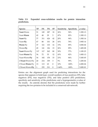
![80
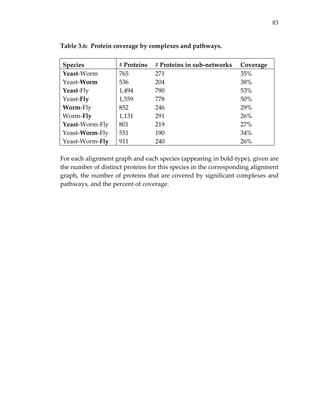
Table 3.1: Cross‐validation for protein cellular process prediction.
Species #Correct #Predictions Success rate
(%)Yeast 114 198 58
Worm 57 95 60
Fly 115 184 63
For each species the table lists the number of correct predictions, the total
number of predictions and the success rate in ten‐fold cross‐validation.
Table 3.2: Cross‐validation results for protein interaction predictions.
Species Sensitivity Specificity p‐value Strate
Yeast 50 77 1.1e‐25 [1]
Worm 43 82 1e‐13 [1]
Fly 23 84 5.3e‐5 [1]
Yeast 9 99 1.2e‐6 [1]+[2]
Worm 10 100 6e‐4 [1]+[2]
Fly 0.4 100 0.5 [1]+[2]
For each species the table lists the specificity and sensitivity of the predictions
in five‐fold cross validation, the significance of the results and the prediction
strategy (see text).](https://image.slidesharecdn.com/0585808f-97e2-4cab-9576-ce24b5c02f6d-150410123344-conversion-gate01/85/SilpaSuthram-Thesis-98-320.jpg)
![85
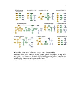
Figure 3.2: Representative conserved network regions.
Shown are conserved clusters [a‐k] and paths [l‐m] identified within the
networks of yeast, worm and fly. Each region contains one or more
overlapping clusters or paths (see Figure 3.3). Proteins from yeast (orange
ovals), worm (green rectangles) or fly (blue hexagons) are connected by
direct (thick link) or indirect (connection via a common network neighbor;
thin link) protein interactions. Horizontal dotted gray links indicate cross‐
species sequence similarity between proteins (similar proteins are
typically placed on the same row of the alignment). Automated layout of
network alignments was performed using a specialized plug‐in to the
Cytoscape software25 as described in Methods.](https://image.slidesharecdn.com/0585808f-97e2-4cab-9576-ce24b5c02f6d-150410123344-conversion-gate01/85/SilpaSuthram-Thesis-103-320.jpg)
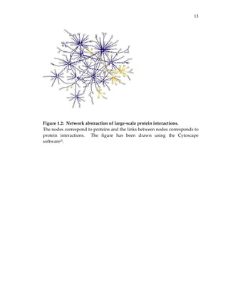
![86
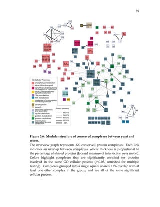
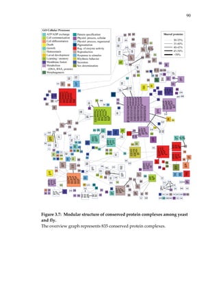
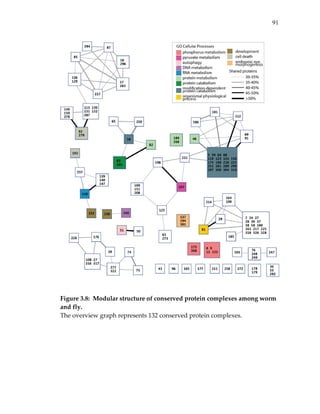
Figure 3.3: Modular structure of conserved clusters among yeast, worm and
fly.
Multiple network alignment revealed 183 conserved clusters, organized into
71 network regions represented by colored squares. Regions group together
clusters that share >15% overlap with at least one other cluster in the group
and are all enriched for the same GO cellular process (p<0.05 with the
enriched processes indicated by color). Cluster ID numbers are given within
each square; numbers are not sequential due to filtering. Solid links indicate
overlaps between different regions, where thickness is proportional to the
percentage of shared proteins (intersection / union). Hashed links indicate
conserved paths that connect clusters together. Labels [a‐k],[m] mark the
network regions exemplified in Figure 3.2.](https://image.slidesharecdn.com/0585808f-97e2-4cab-9576-ce24b5c02f6d-150410123344-conversion-gate01/85/SilpaSuthram-Thesis-104-320.jpg)
![87
Figure 3.4: Verification of predicted interactions by two‐hybrid testing.
[a] 65 pairs of yeast proteins were tested for physical interaction based on their
co‐occurrence within the same conserved cluster and the presence of
orthologous interactions in worm and fly. Each protein pair is listed along
with its position on the agar plates shown in [b] and [c] and the outcome of
the two‐hybrid test. [b] Raw test results are shown, with each protein pair
tested in quadruplicate to ensure reproducibility. Protein 1 vs. 2 of each pair
was used as prey vs. bait, respectively. [c] This negative control reveals
activating baits, which can lead to positive tests without interaction. Protein 2
of each pair was used as bait with an empty pOAD vector as prey. Activating
baits are denoted by “a” in the list of predictions shown in [a]. Positive tests
with weak signal (e.g., A1) and control colonies with marginal activation are
denoted by “?” in the list; colonies D4, E2 and E5 show evidence of possible
contamination and are also marked by a “?”. Discarding the activating baits,
31 out of 60 predictions tested positive overall. A more conservative tally,
disregarding all results marked by a “?”, yields 19 out of 48 positive
predictions.](https://image.slidesharecdn.com/0585808f-97e2-4cab-9576-ce24b5c02f6d-150410123344-conversion-gate01/85/SilpaSuthram-Thesis-105-320.jpg)
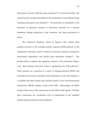
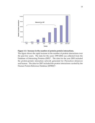
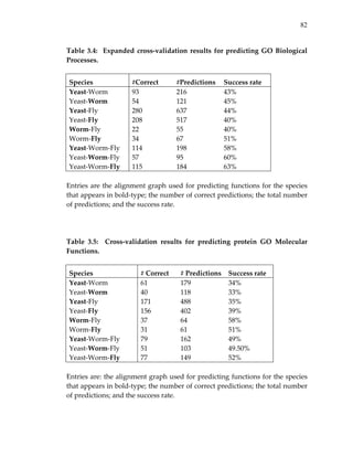
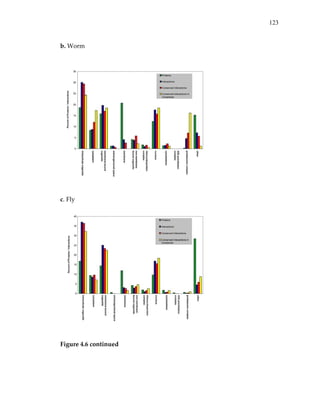
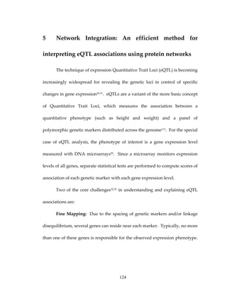
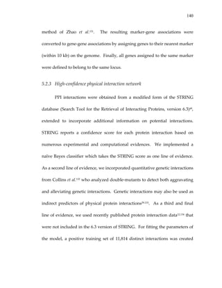
![122
a. Yeast
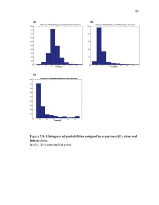
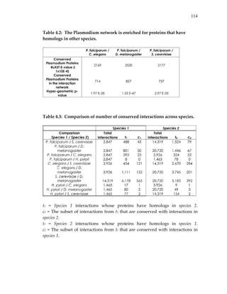
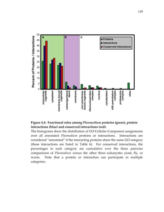
Figure 4.6: Gene Ontology (GO) enrichment among cellular components in
yeast (a), worm (b) ,and fly (c).
These histograms are complementary to Figure 4.4 and indicate the
representation of common cellular components in each species’ genome
(green), set of interactions (blue), conserved interactions (red), and conserved
complexes (yellow). The percentages of conserved interactions are combined
over the separate pairwise comparisons for each species (eg. in panel [a], data
from yeast vs. worm, fly or Plasmodium comparison was used). Note that a
protein or interaction can participate in multiple categories.](https://image.slidesharecdn.com/0585808f-97e2-4cab-9576-ce24b5c02f6d-150410123344-conversion-gate01/85/SilpaSuthram-Thesis-140-320.jpg)
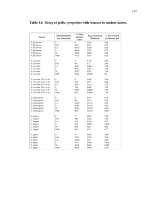
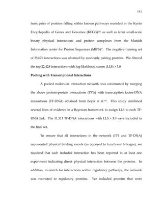
![138
In the case of random walks derived from electric networks, it can be shown
that:
C
C
w j
j = where ∑=
x
xCC
An ergodic chain is called time‐reversible if yxyxyx PwPw = . Thus, in the
case of the random walk derived from an electric circuit,
yxy
y
yx
y
y
y
y
y
yx
x
x
xy
x
xy
x
x
x
xyx Pw
C
C
C
C
C
C
C
C
C
C
C
C
Pw =====
∑∑∑∑
..
As a result, the random walk P is also time‐reversible. Finally, using
the above properties we can show that when a unit current flows into an
electric network at node “a” and leaves at node “b”, then the amount of
current through any intermediary node or edge is proportional to the
expected number of times a random walker will pass through that node or
edge [see Doyle et al.117 for details].
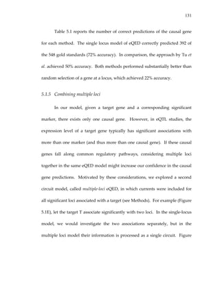
We demonstrate this equivalence using the sample network of Figure
5.1A. Figure 5.1C is the electric network model of the sample network. Here,
we add a new node L which is connected to all the candidate genes in the
locus. The edges connecting L to L1, L2 and L3 have infinite conductance and
for all purposes, L is no different from any of L1, L2 or L3. The conductance](https://image.slidesharecdn.com/0585808f-97e2-4cab-9576-ce24b5c02f6d-150410123344-conversion-gate01/85/SilpaSuthram-Thesis-156-320.jpg)
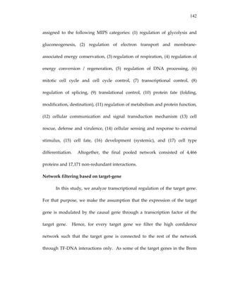

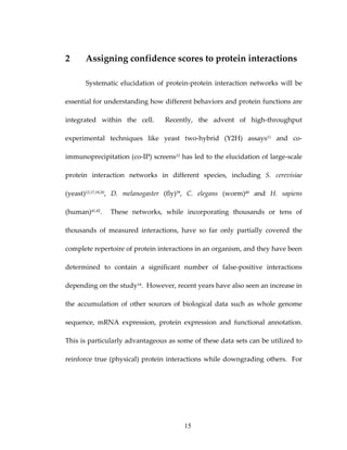
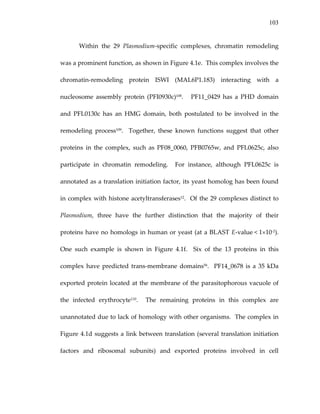
![147
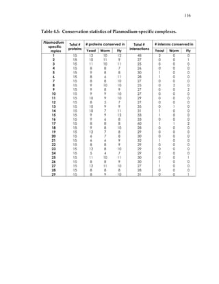
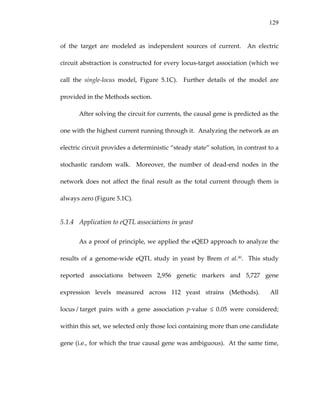
Figure 5.1: Examples of the electrical circuit approach and the eQED model.
[A] Sample network. [B] The “greedy” random walk approach by Tu et al.
[C] The single locus model of eQED. Gene T in the blue hexagon is the target
gene. The locus marked by the red box, containing candidate genes L1, L2
and L3, associates significantly with the target T. The numbers next to the
locus genes corresponds to the number of times the gene was visited in the
random walk approaches or the amount of current through them in the
electric circuit approach. [D] The random walk derived from [C]. [E] The
sample network with two significant loci. [F] The multiple loci model of
eQED.](https://image.slidesharecdn.com/0585808f-97e2-4cab-9576-ce24b5c02f6d-150410123344-conversion-gate01/85/SilpaSuthram-Thesis-165-320.jpg)
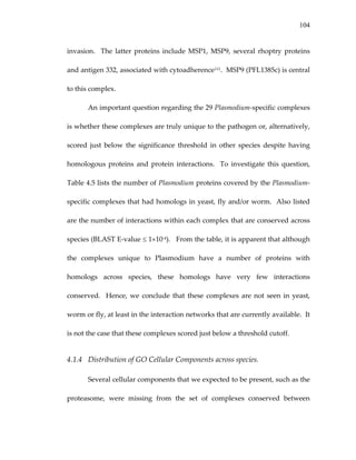
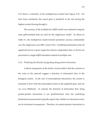
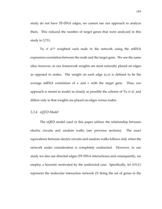
![149
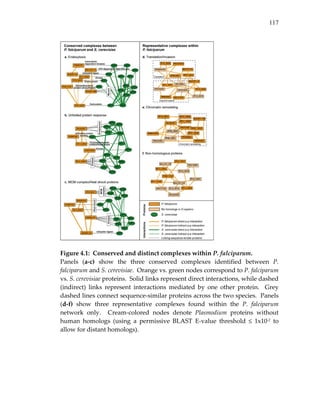
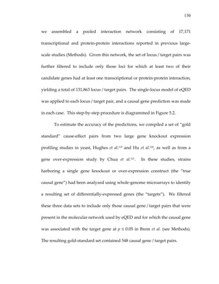
Figure 5.3: Inferred pathways and directionality prediction.
[A] The accuracy of the direction prediction methods. The “gold” standard
set of protein interactions were ranked according to the different metrics and,
the ranks in each approach was plotted as the x‐axis. [B‐D] The regulatory
networks for three example target genes. The nodes colored in shades of red
correspond to predicted causal genes. The intensity of color corresponds to
their p‐value of association with the target.](https://image.slidesharecdn.com/0585808f-97e2-4cab-9576-ce24b5c02f6d-150410123344-conversion-gate01/85/SilpaSuthram-Thesis-167-320.jpg)

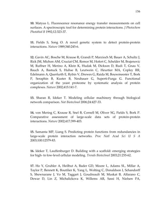
![169
112. Finn RD, Marshall M, Bateman A. iPfam: visualization of protein‐protein
interactions in PDB at domain and amino acid resolutions. Bioinformatics
2005;21:410‐2.
113. Griffiths AJF. Modern genetic analysis : integrating genes and genomes.
New York: W.H. Freeman and Co., 2002:xix, 736 p.
114. Kulp DC, Jagalur M. Causal inference of regulator‐target pairs by gene
mapping of expression phenotypes. BMC Genomics 2006;7:125.
115. Perez‐Enciso M, Quevedo JR, Bahamonde A. Genetical genomics: use all
data. BMC Genomics 2007;8:69.
116. Beyer A, Bandyopadhyay S, Ideker T. Integrating physical and genetic
maps: from genomes to interaction networks. Nat Rev Genet 2007;8:699‐710.
117. Doyle PG, Snell JL. Random walks and electric networks. [Washington,
D.C.]: Mathematical Association of America, 1984:xiii, 159 p.
118. Albert‐László Barabási RA. Emergence of Scaling in Random Networks.
Science 1999;286:509 ‐ 512.
119. Hughes TR, Marton MJ, Jones AR, Roberts CJ, Stoughton R, Armour CD,
Bennett HA, Coffey E, Dai H, He YD, Kidd MJ, King AM, Meyer MR, Slade D,
Lum PY, Stepaniants SB, Shoemaker DD, Gachotte D, Chakraburtty K, Simon
J, Bard M, Friend SH. Functional discovery via a compendium of expression
profiles. Cell 2000;102:109‐26.
120. Hu Z, Killion PJ, Iyer VR. Genetic reconstruction of a functional
transcriptional regulatory network. Nat Genet 2007;39:683‐687.
121. Chua G, Morris QD, Sopko R, Robinson MD, Ryan O, Chan ET, Frey BJ,
Andrews BJ, Boone C, Hughes TR. Identifying transcription factor functions](https://image.slidesharecdn.com/0585808f-97e2-4cab-9576-ce24b5c02f6d-150410123344-conversion-gate01/85/SilpaSuthram-Thesis-187-320.jpg)

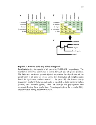
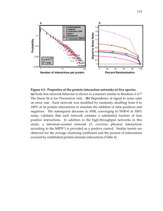
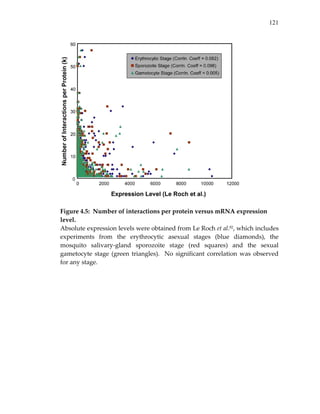
This document is Silpa Suthram's PhD dissertation from the University of California, San Diego. The dissertation examines understanding cellular function through analysis of protein interaction networks. It includes 3 chapters that analyze noise in protein interaction data, perform comparative network analysis across species, and integrate networks to interpret expression quantitative trait loci (eQTL) associations using protein networks. The dissertation was submitted in partial fulfillment of the requirements for a Doctor of Philosophy in Bioinformatics.


![[Medicina] genetica molecular biology of the gene - watson j d , et al (5th e...](https://cdn.slidesharecdn.com/ss_thumbnails/8ounzyuirsojxks4isn9-signature-6ed96f61ba451dd55dc51bcf3f726eb18253d00f9f8650f3e5c1a1a36c1f18b2-poli-140721000012-phpapp01-thumbnail.jpg?width=640&height=640&fit=bounds)


![[H.gerhard vogel, jochen_maas,_alexander_gebauer]_(book_fi.org)](https://cdn.slidesharecdn.com/ss_thumbnails/5bh-131107052403-phpapp01-thumbnail.jpg?width=640&height=640&fit=bounds)


