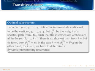
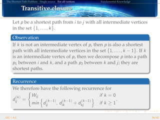
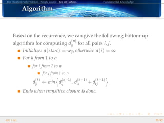
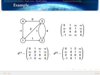
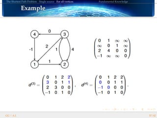
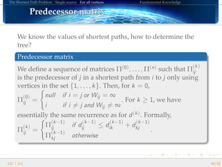
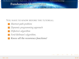
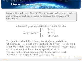
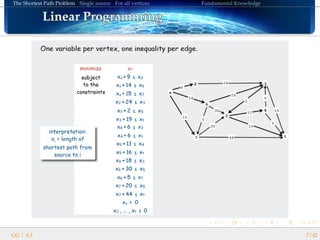
The document discusses shortest path problems in graphs. It introduces the shortest path problem and describes algorithms for finding shortest paths from a single source (Dijkstra's and Bellman-Ford algorithms) and for all vertex pairs (Bellman-Ford algorithm). It also discusses dynamic programming, linear programming formulations, and properties like Bellman's principle of optimality and the existence of a shortest path tree from any starting vertex. Examples are provided to illustrate the algorithms.


![The Shortest Path Problem Single source For all vertices Fundamental Knowledge
AlgorithmAlgorithmAlgorithmAlgorithmAlgorithmAlgorithmAlgorithmAlgorithmAlgorithmAlgorithmAlgorithmAlgorithmAlgorithmAlgorithmAlgorithmAlgorithmAlgorithm
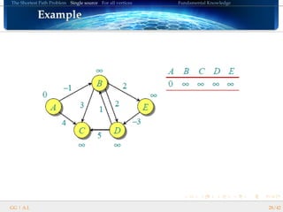
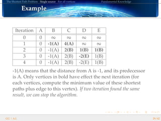
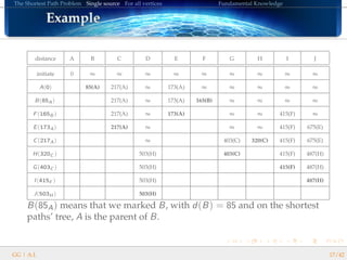
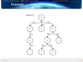
DIJKSTRA’s algorithm follows these steps:
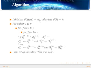
Initialize: d(start) = 0, otherwise d(i) = ∞
At each iteration:
Select the unvisited vertex with smallest non-∞ distance, denoted
a. Set it as visited.
Mark each of the vertices b adjacent to a (its neighbours)
If a neighbour was not marked, set its distance to a’s distance plus
the weight of the edge going to that neighbour.
If it was marked, overwrite its distance if the result is smaller than
its current distance.
i.e. d[b] = min(d[b], d[a] + weight(a, b)).
Ends when we visit the target vertex or no more non-∞
distances.
GG | A.I. 15/42](https://image.slidesharecdn.com/lecture3course-161125164250/85/Shortest-Path-Problem-15-320.jpg)
![The Shortest Path Problem Single source For all vertices Fundamental Knowledge
AlgorithmAlgorithmAlgorithmAlgorithmAlgorithmAlgorithmAlgorithmAlgorithmAlgorithmAlgorithmAlgorithmAlgorithmAlgorithmAlgorithmAlgorithmAlgorithmAlgorithm
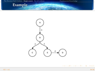
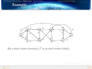
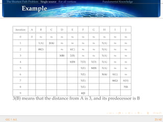
BELLMAN’s algorithm follows these steps:
Initialize: d(start) = 0, otherwise d(i) = ∞
At each iteration:
Select the unvisited vertex which have all its predecessor visited.
Mark each of the vertices b adjacent to a (its neighbours)
If a neighbour was not marked, set its distance to a’s distance plus
the weight of the edge going to that neighbour.
If it was marked, overwrite its distance if the result is smaller than
its current distance.
i.e. d[b] = min(d[b], d[a] + weight(a, b)).
Ends when we visit the target vertex or no more valid vertices.
GG | A.I. 21/42](https://image.slidesharecdn.com/lecture3course-161125164250/85/Shortest-Path-Problem-21-320.jpg)
![The Shortest Path Problem Single source For all vertices Fundamental Knowledge
AlgorithmAlgorithmAlgorithmAlgorithmAlgorithmAlgorithmAlgorithmAlgorithmAlgorithmAlgorithmAlgorithmAlgorithmAlgorithmAlgorithmAlgorithmAlgorithmAlgorithm
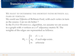
BELLMAN-FORD’s algorithm follows these steps:
Initialize: d(start) = 0, otherwise d(i) = ∞
For i from 1 to |V | − 1 (the diameter of a graph is at most
|V | − 1)
d[b] = min(d[b], d[a] + weight(a, b)) for each edge (u, v) ∈ A
For each edge (u, v) ∈ A, if d[b] > d[a] + weight(a, b) then
report a negative-weight cycle.
GG | A.I. 27/42](https://image.slidesharecdn.com/lecture3course-161125164250/85/Shortest-Path-Problem-27-320.jpg)