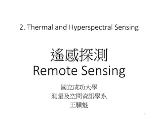
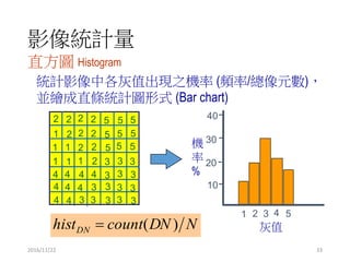
Thermal imaging
TABI-1800, 11:30pm, GSD 15 cm
Natural gas processing facility
and power plant
Alberta, Canada
chimney
Plume of hot gas
chimney
(not in use)
underground
pipe
2
3.
Thermal imaging
• Notdependent on reflected solar radiation
• Can be operated at any time of the day or night
• Operated in 3 – 5 μm or 8 – 14 μm due to
atmospheric effect
• Detectors must be cooled to very low temperature
for maximum sensitivity
Type Abbreviation Useful Spectral Range
Mercury-doped germanium
(汞摻鍺)
Ge:Hg 3 – 14 μm
Indium antimonide
(銻化銦)
InSb 3 – 5 μm
Mercury cadmium telluride
(汞碲化鎘)
HgCdTe (MCT), or “trimetal” 3 – 14 μm
3
4.
Thermal radiation principles
Objectwith temperature
Internal temperature
(kinetic temperature)
Thermal
detectorRadiant temperature
(external temperature)
4
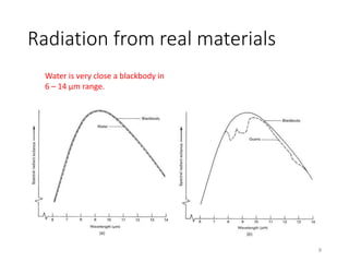
Radiation from realmaterials
• All real materials emit only a fraction of the energy
emitted from a blackbody at the equivalent
temperature.
• Emissivity
• Emissivity can vary with wavelength
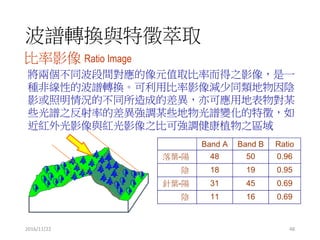
• Emissivity can even vary with temperature
depending on the material
𝜀 λ =
radiant exitance of an oject at a given temperature
radiant exitance of a blackbody at the same temperature
0 < 𝜀 λ < 1
6
7.
Radiation from realmaterials
• Graybody has an
emissivity less than 1 but
is constant at all
wavelengths
• The emissivity of selective
radiator is a function of
wavelength
7
8.
Radiation from realmaterials
Water is very close a blackbody in
6 – 14 μm range.
8
9.
Variations of emissivity
•Material
• Condition and
arrangement of the
materials
• Dry soil (0.95) vs. wet
soil (0.92)
• Loose soil vs.
compacted soil
• Individual tree leaves
(0.96) vs tree crowns
(0.98)
Material
Typical Average
Emissivity over 8 -14 μm
Clear water 0.98 - 0.99
Wet snow 0.98 - 0.99
Human skin 0.97 - 0.99
Rough ice 0.97 - 0.98
Healthy green vegetation 0.96 - 0.99
Wet soil 0.95 - 0.98
Asphaltic concrete 0.94 - 0.97
Brick 0.93 - 0.94
Wood 0.93 - 0.94
Basaltic rock 0.92 - 0.96
Dry mineral soil 0.92 - 0.94
Portland cement concrete 0.90 - 0.94
Paint 0.90 - 0.96
Dry vegetation 0.88 - 0.94
Dry snow 0.85 - 0.90
Granitic rock 0.83 - 0.87
Glass 0.77 - 0.81
Sheet iron (rusted) 0.63 - 0.70
Polished metals 0.16 - 0.21
Aluminum foil 0.03 - 0.07
Highly polished gold 0.02 - 0.03
9
10.
Consideration of spectralrange for
thermal data
• The ambient temperature of earth surface is normally
about .
• This results a peak emission at approximately 9.7 μm.
• Hence, most thermal sensors perform at 8 – 14 μm
range.
• Although it’s a fact that the emissivity of objects can
vary in 8 – 14 μ m, for broad band detectors, the
objects are assumed as graybody.
• Cautions should be exercised when conducting inter-
data comparison.
within-band emissivity of materials in 10.5 – 11.5 μm sensed
by NOAA AVHRR is not the same as those in 10.4 – 12.5 μm
sensed by Landsat TM band 6.
• The 3 – 5 μm range is useful for forest fire mapping.
10
11.
Atmospheric effects
• Withingiven atmospheric window
• atmospheric absorption and scattering tend to make the signals
from ground objects appear colder than they are
• atmospheric emission tends to make objects appear warmer than
they are
11
12.
Interaction of thermalradiation
with terrain elements
𝐸𝐼 = 𝐸𝐴 + 𝐸 𝑅 + 𝐸 𝑇
⇒
𝐸𝐼
𝐸𝐼
=
𝐸𝐴
𝐸𝐼
+
𝐸 𝑅
𝐸𝐼
+
𝐸 𝑇
𝐸𝐼
⇒ 1 = 𝛼 λ + 𝛽 λ + 𝜏 λ
𝐸𝐼 = energy incidnet on surface of terrain element
𝐸𝐴 = component of incident energy absorbed by terrain element
𝐸 𝑅 = component of incident energy reflected by terrain element
𝐸 𝑇 = component of incident energy transmitted by terrain element
𝛼 λ = absorptance of terrain element
𝛽 λ = reflectance of terrain element
𝜏 λ = transmittance of terrain element
For Krichhoff radiation law, the spectral emissivity of an object equals its spectral
absorptance, i.e., “good absorbers are good emitters”, 𝜀 λ = 𝛼 λ .
⇒ 1 = 𝜀 λ + 𝛽 λ + 𝜏 λ
In remote sensing applications, we assume all objects are opaque to thermal radiation.
⇒ 𝟏 = 𝜺 𝝀 + 𝜷 𝝀 The higher an objects’ reflectance, the lower its emissivity;
vice versa. 12
13.
Interaction of thermalradiation
with terrain elements
• Water has negligibly low reflectance in thermal IR
(TIR), so its emissivity is essential 1 for that spectral
range.
• Sheet metal is highly reflective of thermal energy,
so it has an emissivity much less than 1.
• So, the thermal measurement of real materials.
• How to obtain the kinetic temperature from radiant
temperature?
𝑀 = 𝜀𝜎𝑇4
13
14.
Diurnal temperature variation
Quasi-equilibrium
(thechange rate of
temperature is small) High-contrast Cooling
Thermal crossover
(no radiant temperature
difference exists between
two materials)
Variation of temperature
(maximum, minimum,
range, time of maximum
and minimum)
14
15.
Thermal properties
• Thermalconductivity
• A measure of the rate at which heat passes through a material
• EX. Heat passes though metals much faster than though rocks.
• Thermal capacity
• Determines how well a material stores head.
• EX. Water has a very high thermal capacity compared to other
material types.
• Thermal inertia
• A measure of the response of a material to temperature changes.
• It increases with an increase in material conductivity, capacity, and
density.
• In general, materials with high thermal inertia have more uniform
surface temperatures thoughtout the day and night than material
of low thermal inertia.
15
16.
Thermal image (qualitativeuse)
Middleton, Wisconsin
Flying height 600 m, IFOV 5 mrad
Daytime (pm 2:40) Nighttime (pm 9:50)
Lake
(warmer than
surroundings)
Pond
(warmer than surroundings)
HighTemperatureLow
Residential area (no thermal
shadow at night)
Thermal “shadows” are created by
trees due to cooler temperature.
Pavements are warmer than
surroundings at both day and night
16
17.
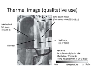
Thermal image (qualitativeuse)
AM 9:40
An ephemeral glacial lake
Middleton, Wisconsin
Flying height 600 m, IFOV 5 mrad
HighTemperatureLow
Lake beach ridge
(fine sandy loam,細砂壤土)
Sod farm
(草皮農場)
Bare soil
Lakebed soil
(silt loam
粉砂壤土)
17
18.
Thermal image (qualitativeuse)
A cattle ranch, Middleton, Wisconsin
Flying height 600 m, IFOV 5 mrad HighTemperatureLow
PM 9:50 AM 1:45
cows
sheet metal
roof
18
19.
Thermal image (qualitativeuse)
Daytime
Quantico, Virginia
IFOV 0.25 mrad, GSD ~0.3 m HighTemperatureLow
cows
shadow?
19
20.
Thermal image (qualitativeuse)
PM 1:50
Oak Creek Power Plant, Wisconsin
Flying height 800 m, IFOV 2.5 mrad HighTemperatureLow
windPlume of
cooling water
Lake Michigan
20
21.
Thermal image (qualitativeuse)
AM 2:00, -4°C (air)
Iowa City
Flying height 460 m, IFOV 1 mrad
HighTemperatureLow
Wind-blown snow
pattern on the
ground
Building heat loss
21
22.
Thermal image (qualitativeuse)
R: band 5 (red)
G: band 3 (green)
B: band 2 (blue)
R: band 12 (thermal IR)
G: band 9 (mid-IR)
B: band 10 (mid-IR)
Zaca Fire
Santa Barbara, California
Autonomous Modular Sensor (AMS), NASA Ikhana UAV
active fire
burned over
area
22
23.
Radiometric calibration ofthermal
images and temperature mapping
• When quantified temperature results are required,
the calibration procedure is a must.
• Two most commonly used calibration methods
• Internal blackbody source referencing
• Air-to-ground correlation
• It is possible to estimate the surface temperature
from the thermal image based on theoretical
atmospheric models with the knowledge of the
atmospheric condition (i.e., temperature, pressure,
CO2 concentration) when the thermal image was
collected.
23
FLIR systems
(not thecompany name)
• Forward-looking infrared (FLIR)
• Compared to traditional system that are 1-D-array- or
scanning-based system, which requires the movement
of the platform and post-processing for image
generation.
• 2D array for real-time application
http://media4.s-nbcnews.com/j/MSNBC/Components/Photo/_new/900501-
airport-thermal-hmed2p.grid-6x2.jpg
https://upload.wikimedia.org/wikipedia/commons/
a/ab/Flickr_-_Official_U.S._Navy_Imagery_-
_Alleged_drug_traffickers_are_arrested_by_Colom
bian_naval_forces..jpg
http://www.guncopter.com/images/gallery/uh-1n.jpg
26
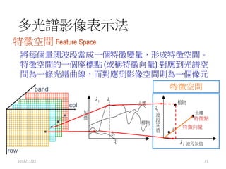
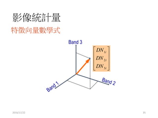
影像分類 Image Classification
2016/11/2251
監督式分類訓練區
將訓練區之像元展繪在
特徵空間,同物類像元
因為光譜特徵相似會聚
集在一起,如右圖。監
督式分類原理即分析計
算訓練區像元在特徵空
間之分布的統計參數,
如中值、範圍及變異量
等,而後利用這些參數
決定其他像元的類別。
Band i
Bandj
W
W
W
W
W
W W
W
W W
W
U
U
U
U
U
U
U
U
UU
U
U
U U
U
U
U
U
U
S
S
S
S
S
S
S
S
S
C
C
C
C
CC
CCC
C
HH
H
H
H H
HH
H
H
H
H
H
H
H
H
H
F
F
F
F
F
F
F
F
F
F
F
FF
F F
F
52.
影像分類 Image Classification
2016/11/2252
最短距離分類法 Minimum-Distance-to-Mean classifier
由各訓練區之群集區域計
算得其中值,而後計算欲
分類像元之光譜值與各中
值距離,以最短距離決定
其類別
Band i
Bandj
W
W
W
W
W
W W
W
W W
W
U
U
U
U
U
U
U
U
UU
U
U
U U
U
U
U
U
U
S
S
S
S
S
S
S
S
S
C
C
C
C
CC
CCC
C
HH
H
H
H H
HH
H
H
H
H
H
H
H
H
H
F
F
F
F
F
F
F
F
F
F
F
FF
F F
F
此分類法只考慮群集分
佈中心,未考量群集分
佈的散佈情形
53.
影像分類 Image Classification
2016/11/2253
平行體分類法 Parallelpiped classifier
由各訓練區之群集分佈區域
之外包平行體劃定類別範圍
,而以欲分類像元之光譜特
徵所在之位置決定其類別
Band i
Bandj
W
W
W
W
W
W W
W
W W
W
U
U
U
U
U
U
U
U
UU
U
U
U U
U
U
U
U
U
S
S
S
S
S
S
S
S
S
C
C
C
C
CC
CCC
C
HH
H
H
H H
HH
H
H
H
H
H
H
H
H
H
F
F
F
F
F
F
F
F
F
F
F
FF
F F
F
同時考慮了群集分佈中心
及散佈,但外包平行體只
是群集散佈情形初步的描
述,而且常有重疊情形,
會產生分類上的困擾
54.
影像分類 Image Classification
2016/11/2254
高斯最似分類法 Gaussian Maximum Likelihood classifier
假設訓練區之群集為高斯正
常分佈,應用 Maximum Likelihood
理論決定群集分佈之參數,
如此則可依 Bayes Theorem 計算
欲分類之像元值屬於各群集
之機率,而以最高機率決定
其所屬之類別
Band i
Bandj
W
W
W
W
W
W W
W
W W
W
U
U
U
U
U
U
U
U
UU
U
U
U U
U
U
U
U
U
S
S
S
S
S
S
S
S
S
C
C
C
C
CC
CCC
C
HH
H
H
H H
HH
H
H
H
H
H
H
H
H
H
F
F
F
F
F
F
F
F
F
F
F
FF
F F
F
等機率線
無上述兩種分類法之缺
點,是為目前最常用的
分類法
分類精度評估
2016/11/22 63
隨機分類正確率
Reference Data(Known Cover Types)
W S F U C H Row Total
W 480*485 68*485 356*485 248*485 402*485 438*485 485
S 480*72 68*72 356*72 248*72 402*72 438*72 72
F 480*353 68*353 356*353 248*353 402*353 438*353 353
U 480*142 68*142 356*142 248*142 402*142 438*142 142
C 480*459 68*459 356*459 248*459 402*459 438*459 459
H 480*481 68*481 356*481 248*481 402*481 438*481 481
ClassificationData
Col. Total 480 68 356 248 402 438 1992
2
1
N
xx
r
i
ii
)(
totalgrand
entriesdiagonalofsum
agreementchance
64.
分類精度評估
2016/11/22 64
793776
1674
1992
1
1
r
i
ii
r
i
ii
xx
x
N
)(
Reference Data(Known Cover Types)
W S F U C H Row Total
W 480 0 5 0 0 0 485
S 0 52 0 20 0 0 72
F 0 0 313 40 0 0 353
U 0 16 0 126 0 0 142
C 0 0 0 38 342 79 459
H 0 0 38 24 60 359 481
ClassificationData
Col. Total 480 68 356 248 402 438 1992
84.019921674OA
%.
.
..
CA-1
CA-OA
ˆ 80800
2001
200840
計算結果
2001992793776 2
.CA