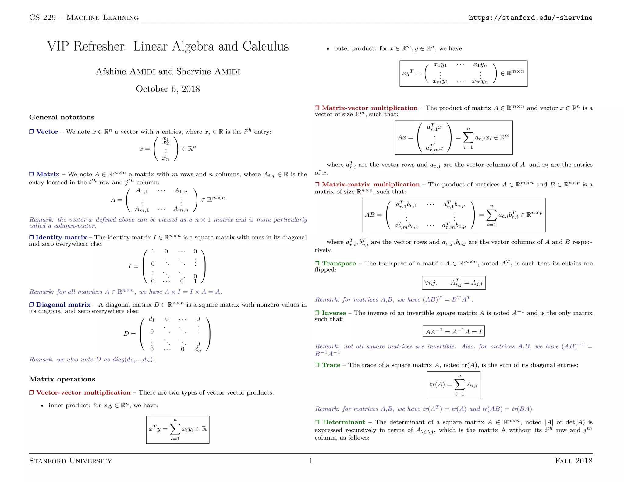
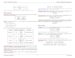
This document provides an overview of key linear algebra and calculus concepts for machine learning, including: 1) Notations for vectors, matrices, and operations like matrix multiplication and transposition. 2) Common matrix properties such as symmetry, positive semi-definiteness, eigenvalues, and singular value decomposition. 3) Derivatives used in calculus on matrices, including the gradient and Hessian of functions with respect to vectors and matrices.

1. CS 229 – Machine Learning https://stanford.edu/~shervine
VIP Refresher: Linear Algebra and Calculus
Afshine Amidi and Shervine Amidi
October 6, 2018
General notations
r Vector – We note x ∈ Rn a vector with n entries, where xi ∈ R is the ith entry:
x =
x1
x2
.
.
.
xn
!
∈ Rn
r Matrix – We note A ∈ Rm×n a matrix with m rows and n columns, where Ai,j ∈ R is the
entry located in the ith row and jth column:
A =
A1,1 · · · A1,n
.
.
.
.
.
.
Am,1 · · · Am,n
!
∈ Rm×n
Remark: the vector x defined above can be viewed as a n × 1 matrix and is more particularly
called a column-vector.
r Identity matrix – The identity matrix I ∈ Rn×n is a square matrix with ones in its diagonal
and zero everywhere else:
I =



1 0 · · · 0
0
...
...
.
.
.
.
.
.
...
... 0
0 · · · 0 1



Remark: for all matrices A ∈ Rn×n, we have A × I = I × A = A.
r Diagonal matrix – A diagonal matrix D ∈ Rn×n is a square matrix with nonzero values in
its diagonal and zero everywhere else:
D =



d1 0 · · · 0
0
...
...
.
.
.
.
.
.
...
... 0
0 · · · 0 dn



Remark: we also note D as diag(d1,...,dn).
Matrix operations
r Vector-vector multiplication – There are two types of vector-vector products:
• inner product: for x,y ∈ Rn, we have:
xT
y =
n
X
i=1
xiyi ∈ R
• outer product: for x ∈ Rm, y ∈ Rn, we have:
xyT
=
x1y1 · · · x1yn
.
.
.
.
.
.
xmy1 · · · xmyn
∈ Rm×n
r Matrix-vector multiplication – The product of matrix A ∈ Rm×n and vector x ∈ Rn is a
vector of size Rm, such that:
Ax =


aT
r,1x
.
.
.
aT
r,mx

 =
n
X
i=1
ac,ixi ∈ Rm
where aT
r,i are the vector rows and ac,j are the vector columns of A, and xi are the entries
of x.
r Matrix-matrix multiplication – The product of matrices A ∈ Rm×n and B ∈ Rn×p is a
matrix of size Rn×p, such that:
AB =


aT
r,1bc,1 · · · aT
r,1bc,p
.
.
.
.
.
.
aT
r,mbc,1 · · · aT
r,mbc,p

 =
n
X
i=1
ac,ibT
r,i ∈ Rn×p
where aT
r,i, bT
r,i are the vector rows and ac,j, bc,j are the vector columns of A and B respec-
tively.
r Transpose – The transpose of a matrix A ∈ Rm×n, noted AT , is such that its entries are
flipped:
∀i,j, AT
i,j = Aj,i
Remark: for matrices A,B, we have (AB)T = BT AT .
r Inverse – The inverse of an invertible square matrix A is noted A−1 and is the only matrix
such that:
AA−1
= A−1
A = I
Remark: not all square matrices are invertible. Also, for matrices A,B, we have (AB)−1 =
B−1A−1
r Trace – The trace of a square matrix A, noted tr(A), is the sum of its diagonal entries:
tr(A) =
n
X
i=1
Ai,i
Remark: for matrices A,B, we have tr(AT ) = tr(A) and tr(AB) = tr(BA)
r Determinant – The determinant of a square matrix A ∈ Rn×n, noted |A| or det(A) is
expressed recursively in terms of Ai,j, which is the matrix A without its ith row and jth
column, as follows:
Stanford University 1 Fall 2018

2. CS 229 – Machine Learning https://stanford.edu/~shervine
det(A) = |A| =
n
X
j=1
(−1)i+j
Ai,j|Ai,j|
Remark: A is invertible if and only if |A| 6= 0. Also, |AB| = |A||B| and |AT | = |A|.
Matrix properties
r Symmetric decomposition – A given matrix A can be expressed in terms of its symmetric
and antisymmetric parts as follows:
A =
A + AT
2
| {z }
Symmetric
+
A − AT
2
| {z }
Antisymmetric
r Norm – A norm is a function N : V −→ [0, + ∞[ where V is a vector space, and such that
for all x,y ∈ V , we have:
• N(x + y) 6 N(x) + N(y)
• N(ax) = |a|N(x) for a scalar
• if N(x) = 0, then x = 0
For x ∈ V , the most commonly used norms are summed up in the table below:
Norm Notation Definition Use case
Manhattan, L1 ||x||1
n
X
i=1
|xi| LASSO regularization
Euclidean, L2 ||x||2
v
u
u
t
n
X
i=1
x2
i Ridge regularization
p-norm, Lp ||x||p
n
X
i=1
xp
i
!1
p
Hölder inequality
Infinity, L∞ ||x||∞ max
i
|xi| Uniform convergence
r Linearly dependence – A set of vectors is said to be linearly dependent if one of the vectors
in the set can be defined as a linear combination of the others.
Remark: if no vector can be written this way, then the vectors are said to be linearly independent.
r Matrix rank – The rank of a given matrix A is noted rank(A) and is the dimension of the
vector space generated by its columns. This is equivalent to the maximum number of linearly
independent columns of A.
r Positive semi-definite matrix – A matrix A ∈ Rn×n is positive semi-definite (PSD) and
is noted A 0 if we have:
A = AT
and ∀x ∈ Rn
, xT
Ax 0
Remark: similarly, a matrix A is said to be positive definite, and is noted A 0, if it is a PSD
matrix which satisfies for all non-zero vector x, xT Ax 0.
r Eigenvalue, eigenvector – Given a matrix A ∈ Rn×n, λ is said to be an eigenvalue of A if
there exists a vector z ∈ Rn{0}, called eigenvector, such that we have:
Az = λz
r Spectral theorem – Let A ∈ Rn×n. If A is symmetric, then A is diagonalizable by a real
orthogonal matrix U ∈ Rn×n. By noting Λ = diag(λ1,...,λn), we have:
∃Λ diagonal, A = UΛUT
r Singular-value decomposition – For a given matrix A of dimensions m × n, the singular-
value decomposition (SVD) is a factorization technique that guarantees the existence of U m×m
unitary, Σ m × n diagonal and V n × n unitary matrices, such that:
A = UΣV T
Matrix calculus
r Gradient – Let f : Rm×n → R be a function and A ∈ Rm×n be a matrix. The gradient of f
with respect to A is a m × n matrix, noted ∇Af(A), such that:
∇Af(A)
i,j
=
∂f(A)
∂Ai,j
Remark: the gradient of f is only defined when f is a function that returns a scalar.
r Hessian – Let f : Rn → R be a function and x ∈ Rn be a vector. The hessian of f with
respect to x is a n × n symmetric matrix, noted ∇2
xf(x), such that:
∇2
xf(x)
i,j
=
∂2f(x)
∂xi∂xj
Remark: the hessian of f is only defined when f is a function that returns a scalar.
r Gradient operations – For matrices A,B,C, the following gradient properties are worth
having in mind:
∇Atr(AB) = BT
∇AT f(A) = (∇Af(A))T
∇Atr(ABAT
C) = CAB + CT
ABT
∇A|A| = |A|(A−1
)T
Stanford University 2 Fall 2018