7.3
Purpose & Overview
•Develop understanding of generating samples from a
specified distribution as input to a simulation model.
• Illustrate some widely-used techniques for generating
random variates:
• Inverse-transform technique
• Acceptance-rejection technique
• Special properties
Prof. Dr. Mesut Güneş ▪ Ch. 7 Random-Variate Generation
4.
7.4
Preparation
• It isassumed that a source of uniform [0,1] random
numbers exists.
• Linear Congruential Method (LCM)
• Random numbers R, R1, R2, … with
• PDF
• CDF
Prof. Dr. Mesut Güneş ▪ Ch. 7 Random-Variate Generation
⎩
⎨
⎧ ≤
≤
=
otherwise
0
1
0
1
)
(
x
x
fR
⎪
⎩
⎪
⎨
⎧
>
≤
≤
<
=
1
1
1
0
0
0
)
(
x
x
x
x
x
FR
0 1
f(x)
x
0 1
F(x)
x
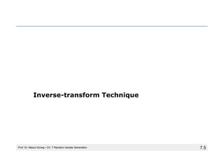
7.6
Inverse-transform Technique
• Theconcept:
• For CDF function: r = F(x)
• Generate r from uniform (0,1), a.k.a U(0,1)
• Find x, x = F-1(r)
Prof. Dr. Mesut Güneş ▪ Ch. 7 Random-Variate Generation
r1
x1
r = F(x)
x
F(x)
1
r1
x1
r = F(x)
x
F(x)
1
r2
x2
7.
7.7
Inverse-transform Technique
• Theinverse-transform technique can be used in principle
for any distribution.
• Most useful when the CDF F(x) has an inverse F -1(x)
which is easy to compute.
• Required steps
1. Compute the CDF of the desired random variable X
2. Set F(X) = R on the range of X
3. Solve the equation F(X) = R for X in terms of R
4. Generate uniform random numbers R1, R2, R3, ... and compute
the desired random variate by Xi = F-1(Ri)
Prof. Dr. Mesut Güneş ▪ Ch. 7 Random-Variate Generation
8.
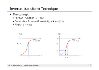
7.8
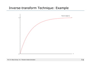
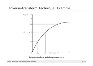
Inverse-transform Technique: Example
•Exponential Distribution
• PDF
• CDF
• To generate X1, X2, X3 …
Prof. Dr. Mesut Güneş ▪ Ch. 7 Random-Variate Generation
x
e
x
f λ
λ −
=
)
(
x
e
x
F λ
−
−
=1
)
(
)
(
)
1
ln(
)
1
ln(
)
1
ln(
1
1
1
R
F
X
R
X
R
X
R
X
R
e
R
e
X
X
−
−
−
=
−
−
=
−
−
=
−
=
−
−
=
=
−
λ
λ
λ
λ
λ
• Simplification
• Since R and (1-R) are uniformly
distributed on [0,1]
λ
)
ln(R
X −
=
7.11
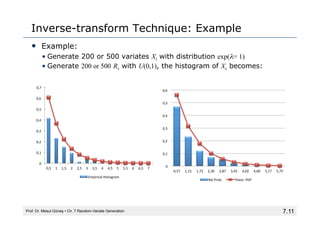
Inverse-transform Technique: Example
•Example:
• Generate 200 or 500 variates Xi with distribution exp(λ= 1)
• Generate 200 or 500 Rs with U(0,1), the histogram of Xs becomes:
Prof. Dr. Mesut Güneş ▪ Ch. 7 Random-Variate Generation
0
0,1
0,2
0,3
0,4
0,5
0,6
0,7
0,5
1
1,5
2
2,5
3
3,5
4
4,5
5
5,5
6
6,5
7
Empirical
Histogram
0
0,1
0,2
0,3
0,4
0,5
0,6
0,57
1,15
1,72
2,30
2,87
3,45
4,02
4,60
5,17
5,75
Rel
Prob.
Theor.
PDF
12.
7.12
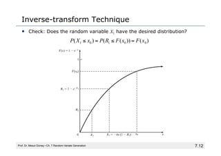
Inverse-transform Technique
• Check:Does the random variable X1 have the desired distribution?
Prof. Dr. Mesut Güneş ▪ Ch. 7 Random-Variate Generation
)
(
))
(
(
)
( 0
0
1
0
1 x
F
x
F
R
P
x
X
P =
≤
=
≤
13.
7.13
Inverse-transform Technique:
Other Distributions
•Examples of other distributions for which inverse CDF
works are:
• Uniform distribution
• Weibull distribution
• Triangular distribution
Prof. Dr. Mesut Güneş ▪ Ch. 7 Random-Variate Generation
14.
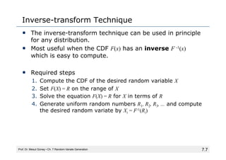
7.14
Inverse-transform Technique:
Uniform Distribution
•Random variable X uniformly distributed over [a, b]
Prof. Dr. Mesut Güneş ▪ Ch. 7 Random-Variate Generation
)
(
)
(
)
(
a
b
R
a
X
a
b
R
a
X
R
a
b
a
X
R
X
F
−
+
=
−
=
−
=
−
−
=
15.
7.15
Inverse-transform Technique:
Weibull Distribution
()β
α
x
e
X
F
−
−
=1
)
(
( )
( )
( )
β
β β
β
β
β
β
β
α
α
α
α
α
β
α
β
α
)
1
ln(
)
1
ln(
)
1
ln(
)
1
ln(
)
1
ln(
1
1
)
(
R
X
R
X
R
X
R
X
R
R
e
R
e
R
X
F
X
X
X
−
−
⋅
=
−
⋅
−
=
−
⋅
−
=
−
−
=
−
=
−
−
=
=
−
=
−
−
Prof. Dr. Mesut Güneş ▪ Ch. 7 Random-Variate Generation
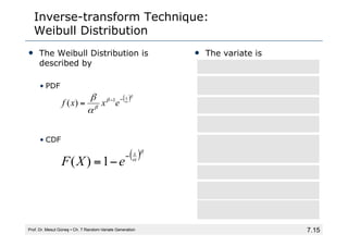
• The Weibull Distribution is
described by
• PDF
• CDF
• The variate is
( )β
α
β
β
α
β x
e
x
x
f
−
−
= 1
)
(
16.
7.16
Inverse-transform Technique:
Triangular Distribution
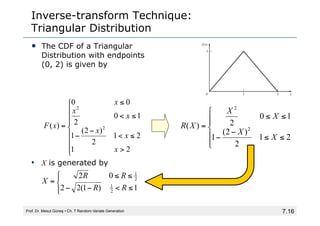
•The CDF of a Triangular
Distribution with endpoints
(0, 2) is given by
• X is generated by
Prof. Dr. Mesut Güneş ▪ Ch. 7 Random-Variate Generation
⎪
⎩
⎪
⎨
⎧
≤
<
−
−
≤
≤
=
1
)
1
(
2
2
0
2
2
1
2
1
R
R
R
R
X
⎪
⎪
⎩
⎪
⎪
⎨
⎧
≤
≤
−
−
≤
≤
=
2
1
2
)
2
(
1
1
0
2
)
( 2
2
X
X
X
X
X
R
⎪
⎪
⎪
⎩
⎪
⎪
⎪
⎨
⎧
>
≤
<
−
−
≤
<
≤
=
2
1
2
1
2
)
2
(
1
1
0
2
0
0
)
( 2
2
x
x
x
x
x
x
x
F
17.
7.17
Inverse-transform Technique:
Empirical ContinuousDistributions
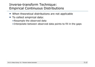
• When theoretical distributions are not applicable
• To collect empirical data:
• Resample the observed data
• Interpolate between observed data points to fill in the gaps
Prof. Dr. Mesut Güneş ▪ Ch. 7 Random-Variate Generation
18.
7.18
Inverse-transform Technique:
Empirical ContinuousDistributions
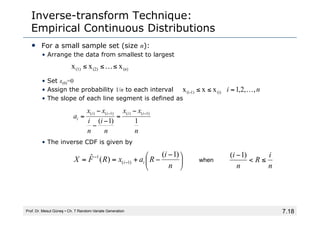
• For a small sample set (size n):
• Arrange the data from smallest to largest
• Set x(0)=0
• Assign the probability 1/n to each interval
• The slope of each line segment is defined as
• The inverse CDF is given by
Prof. Dr. Mesut Güneş ▪ Ch. 7 Random-Variate Generation
(n)
(2)
(1) x
x
x ≤
…
≤
≤
n
i ,
,
2
,
1
x
x
x (i)
1)
-
(i …
=
≤
≤
⎟
⎠
⎞
⎜
⎝
⎛ −
−
+
=
= −
−
n
i
R
a
x
R
F
X i
i
)
1
(
)
(
ˆ
)
1
(
1
n
x
x
n
i
n
i
x
x
a
i
i
i
i
i
1
)
1
(
)
1
(
)
(
)
1
(
)
( −
− −
=
−
−
−
=
n
i
R
n
i
≤
<
− )
1
(
when
19.
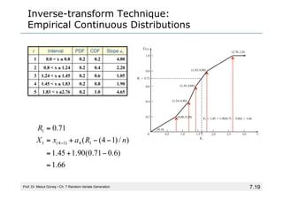
7.19
Inverse-transform Technique:
Empirical ContinuousDistributions
Prof. Dr. Mesut Güneş ▪ Ch. 7 Random-Variate Generation
i Interval PDF CDF Slope ai
1 0.0 < x ≤ 0.8 0.2 0.2 4.00
2 0.8 < x ≤ 1.24 0.2 0.4 2.20
3 1.24 < x ≤ 1.45 0.2 0.6 1.05
4 1.45 < x ≤ 1.83 0.2 0.8 1.90
5 1.83 < x ≤2.76 0.2 1.0 4.65
66
.
1
)
6
.
0
71
.
0
(
90
.
1
45
.
1
)
/
)
1
4
(
(
71
.
0
1
4
)
1
4
(
1
1
=
−
+
=
−
−
+
=
=
− n
R
a
x
X
R
20.
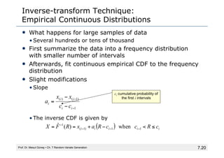
7.20
Inverse-transform Technique:
Empirical ContinuousDistributions
• What happens for large samples of data
• Several hundreds or tens of thousand
• First summarize the data into a frequency distribution
with smaller number of intervals
• Afterwards, fit continuous empirical CDF to the frequency
distribution
• Slight modifications
• Slope
• The inverse CDF is given by
Prof. Dr. Mesut Güneş ▪ Ch. 7 Random-Variate Generation
1
)
1
(
)
(
−
−
−
−
=
i
i
i
i
i
c
c
x
x
a
( ) i
i
i
i
i c
R
c
c
R
a
x
R
F
X ≤
<
−
+
=
= −
−
−
−
1
1
)
1
(
1
when
)
(
ˆ
ci cumulative probability of
the first i intervals
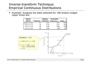
21.
7.21
Inverse-transform Technique:
Empirical ContinuousDistributions
• Example: Suppose the data collected for 100 broken-widget
repair times are:
Prof. Dr. Mesut Güneş ▪ Ch. 7 Random-Variate Generation
Interval
(Hours) Frequency
Relative
Frequency
Cumulative
Frequency, ci Slope, ai
0.25 ≤ x ≤ 0.5 31 0.31 0.31 0.81
0.5 ≤ x ≤ 1.0 10 0.10 0.41 5.00
1.0 ≤ x ≤ 1.5 25 0.25 0.66 2.00
1.5 ≤ x ≤ 2.0 34 0.34 1.00 1.47
Consider R1 = 0.83:
c3 = 0.66 < R1 < c4 = 1.00
X1 = x(4-1) + a4(R1 – c(4-1))
= 1.5 + 1.47(0.83-0.66)
= 1.75
22.
7.22
Inverse-transform Technique:
Empirical ContinuousDistributions
• Problems with empirical distributions
• The data in the previous example is restricted in the range
0.25 ≤ X ≤ 2.0
• The underlying distribution might have a wider range
• Thus, try to find a theoretical distribution
• Hints for building empirical distributions based on
frequency tables
• It is recommended to use relatively short intervals
• Number of bins increase
• This will result in a more accurate estimate
Prof. Dr. Mesut Güneş ▪ Ch. 7 Random-Variate Generation
23.
7.23
Inverse-transform Technique:
Continuous Distributions
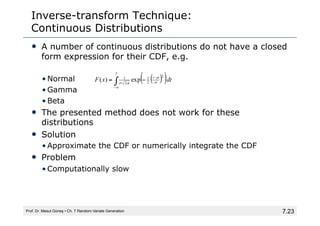
•A number of continuous distributions do not have a closed
form expression for their CDF, e.g.
• Normal
• Gamma
• Beta
• The presented method does not work for these
distributions
• Solution
• Approximate the CDF or numerically integrate the CDF
• Problem
• Computationally slow
Prof. Dr. Mesut Güneş ▪ Ch. 7 Random-Variate Generation
( )
( )dt
x
F
x
t
exp
)
(
2
2
1
2
1
∫∞
−
−
−
= σ
µ
π
σ
24.
7.24
Inverse-transform Technique:
Discrete Distribution
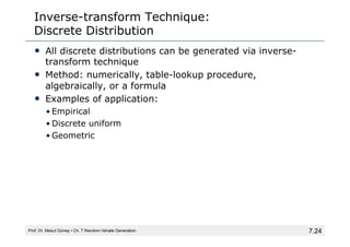
•All discrete distributions can be generated via inverse-
transform technique
• Method: numerically, table-lookup procedure,
algebraically, or a formula
• Examples of application:
• Empirical
• Discrete uniform
• Geometric
Prof. Dr. Mesut Güneş ▪ Ch. 7 Random-Variate Generation
25.
7.25
Inverse-transform Technique:
Discrete Distribution
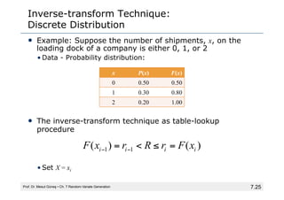
•Example: Suppose the number of shipments, x, on the
loading dock of a company is either 0, 1, or 2
• Data - Probability distribution:
• The inverse-transform technique as table-lookup
procedure
• Set X = xi
Prof. Dr. Mesut Güneş ▪ Ch. 7 Random-Variate Generation
)
(
)
( 1
1 i
i
i
i x
F
r
R
r
x
F =
≤
<
= −
−
x P(x) F(x)
0 0.50 0.50
1 0.30 0.80
2 0.20 1.00
26.
7.26
Inverse-transform Technique:
Discrete Distribution
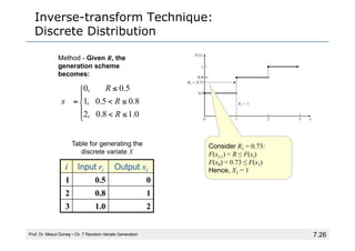
Prof.Dr. Mesut Güneş ▪ Ch. 7 Random-Variate Generation
0
.
1
8
.
0
8
.
0
5
.
0
5
.
0
,
2
,
1
,
0
≤
<
≤
<
≤
⎪
⎩
⎪
⎨
⎧
=
R
R
R
x
Method - Given R, the
generation scheme
becomes:
i Input ri Output xi
1 0.5 0
2 0.8 1
3 1.0 2
Table for generating the
discrete variate X
Consider R1 = 0.73:
F(xi-1) < R ≤ F(xi)
F(x0) < 0.73 ≤ F(x1)
Hence, X1 = 1
0.8
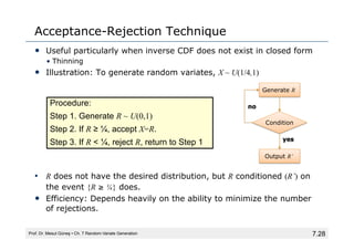
7.28
Acceptance-Rejection Technique
• Usefulparticularly when inverse CDF does not exist in closed form
• Thinning
• Illustration: To generate random variates, X ~ U(1/4,1)
• R does not have the desired distribution, but R conditioned (R’) on
the event {R ≥ ¼} does.
• Efficiency: Depends heavily on the ability to minimize the number
of rejections.
Prof. Dr. Mesut Güneş ▪ Ch. 7 Random-Variate Generation
Procedure:
Step 1. Generate R ~ U(0,1)
Step 2. If R ≥ ¼, accept X=R.
Step 3. If R < ¼, reject R, return to Step 1
Generate R
Condition
Output R’
yes
no
29.
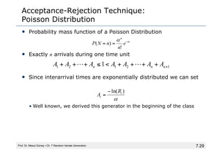
7.29
Acceptance-Rejection Technique:
Poisson Distribution
•Probability mass function of a Poisson Distribution
• Exactly n arrivals during one time unit
• Since interarrival times are exponentially distributed we can set
• Well known, we derived this generator in the beginning of the class
Prof. Dr. Mesut Güneş ▪ Ch. 7 Random-Variate Generation
α
α −
=
= e
n
n
N
P
n
!
)
(
1
2
1
2
1 1 +
+
+
+
+
<
≤
+
+
+ n
n
n A
A
A
A
A
A
A
α
)
ln( i
i
R
A
−
=
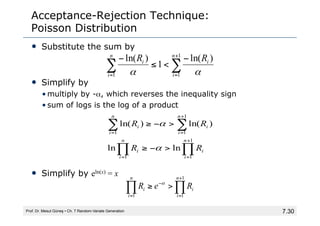
30.
7.30
Acceptance-Rejection Technique:
Poisson Distribution
•Substitute the sum by
• Simplify by
• multiply by -α, which reverses the inequality sign
• sum of logs is the log of a product
• Simplify by eln(x) = x
Prof. Dr. Mesut Güneş ▪ Ch. 7 Random-Variate Generation
∏
∏
+
=
−
=
>
≥
1
1
1
n
i
i
n
i
i R
e
R α
∑
∑
+
=
=
−
<
≤
− 1
1
1
)
ln(
1
)
ln( n
i
i
n
i
i R
R
α
α
∏
∏
∑
∑
+
=
=
+
=
=
>
−
≥
>
−
≥
1
1
1
1
1
1
ln
ln
)
ln(
)
ln(
n
i
i
n
i
i
n
i
i
n
i
i
R
R
R
R
α
α
31.
7.31
Acceptance-Rejection Technique:
Poisson Distribution
•Procedure of generating a Poisson random variate N is as
follows
1. Set n=0, P=1
2. Generate a random number Rn+1, and replace P by P x Rn+1
3. If P < exp(-α), then accept N=n
• Otherwise, reject the current n, increase n by one, and return
to step 2.
Prof. Dr. Mesut Güneş ▪ Ch. 7 Random-Variate Generation
32.
7.32
Acceptance-Rejection Technique:
Poisson Distribution
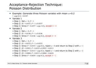
•Example: Generate three Poisson variates with mean α=0.2
• exp(-0.2) = 0.8187
• Variate 1
• Step 1: Set n = 0, P = 1
• Step 2: R1 = 0.4357, P = 1 x 0.4357
• Step 3: Since P = 0.4357 < exp(- 0.2), accept N = 0
• Variate 2
• Step 1: Set n = 0, P = 1
• Step 2: R1 = 0.4146, P = 1 x 0.4146
• Step 3: Since P = 0.4146 < exp(-0.2), accept N = 0
• Variate 3
• Step 1: Set n = 0, P = 1
• Step 2: R1 = 0.8353, P = 1 x 0.8353
• Step 3: Since P = 0.8353 > exp(-0.2), reject n = 0 and return to Step 2 with n = 1
• Step 2: R2 = 0.9952, P = 0.8353 x 0.9952 = 0.8313
• Step 3: Since P = 0.8313 > exp(-0.2), reject n = 1 and return to Step 2 with n = 2
• Step 2: R3 = 0.8004, P = 0.8313 x 0.8004 = 0.6654
• Step 3: Since P = 0.6654 < exp(-0.2), accept N = 2
Prof. Dr. Mesut Güneş ▪ Ch. 7 Random-Variate Generation
33.
7.33
Acceptance-Rejection Technique:
Poisson Distribution
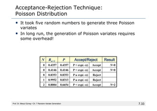
•It took five random numbers to generate three Poisson
variates
• In long run, the generation of Poisson variates requires
some overhead!
Prof. Dr. Mesut Güneş ▪ Ch. 7 Random-Variate Generation
N Rn+1 P Accept/Reject Result
0 0.4357 0.4357 P < exp(- α) Accept N=0
0 0.4146 0.4146 P < exp(- α) Accept N=0
0 0.8353 0.8353 P ≥ exp(- α) Reject
1 0.9952 0.8313 P ≥ exp(- α) Reject
2 0.8004 0.6654 P < exp(- α) Accept N=2
7.35
Special Properties
• Basedon features of particular family of probability
distributions
• For example:
• Direct Transformation for normal and lognormal distributions
• Convolution
Prof. Dr. Mesut Güneş ▪ Ch. 7 Random-Variate Generation
36.
7.36
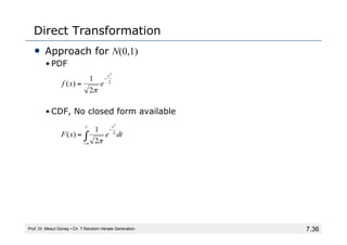
Direct Transformation
• Approachfor N(0,1)
• PDF
• CDF, No closed form available
Prof. Dr. Mesut Güneş ▪ Ch. 7 Random-Variate Generation
∫∞
−
−
=
x t
dt
e
x
F 2
2
2
1
)
(
π
2
2
2
1
)
(
x
e
x
f
−
=
π
37.
7.37
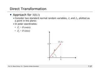
Direct Transformation
• Approachfor N(0,1)
• Consider two standard normal random variables, Z1 and Z2, plotted as
a point in the plane:
• In polar coordinates:
• Z1 = B cos(α)
• Z2 = B sin(α)
Prof. Dr. Mesut Güneş ▪ Ch. 7 Random-Variate Generation
(Z1,Z2)
α
Z1
Z2
B
38.
7.38
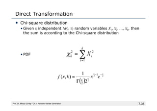
Direct Transformation
• Chi-squaredistribution
• Given k independent N(0, 1) random variables X1, X2, …, Xk, then
the sum is according to the Chi-square distribution
• PDF
Prof. Dr. Mesut Güneş ▪ Ch. 7 Random-Variate Generation
∑
=
=
k
i
i
k X
1
2
2
χ
( )
2
2
2
1
2 2
1
)
,
(
x
k
k e
x
k
x
f
k
−
−
Γ
=
39.
7.39
Direct Transformation
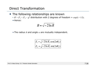
• Thefollowing relationships are known
• B2 = Z2
1 + Z2
2 ~ χ2 distribution with 2 degrees of freedom = exp(λ = 1/2).
• Hence:
• The radius B and angle α are mutually independent.
Prof. Dr. Mesut Güneş ▪ Ch. 7 Random-Variate Generation
R
B ln
2
−
=
)
2
sin(
ln
2
)
2
cos(
ln
2
2
1
2
2
1
1
R
R
Z
R
R
Z
π
π
−
=
−
=
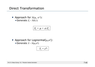
40.
7.40
Direct Transformation
• Approachfor N(µ, σ 2):
• Generate Zi ~ N(0,1)
• Approach for Lognormal(µ,σ2):
• Generate X ~ N(µ,σ2)
Prof. Dr. Mesut Güneş ▪ Ch. 7 Random-Variate Generation
Yi = eXi
Xi = µ + σ Zi
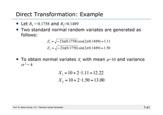
41.
7.41
Direct Transformation: Example
•Let R1 = 0.1758 and R2=0.1489
• Two standard normal random variates are generated as
follows:
• To obtain normal variates Xi with mean µ=10 and variance
σ 2 = 4
Prof. Dr. Mesut Güneş ▪ Ch. 7 Random-Variate Generation
50
.
1
)
1489
.
0
2
sin(
)
1758
.
0
ln(
2
11
.
1
)
1489
.
0
2
cos(
)
1758
.
0
ln(
2
2
1
=
−
=
=
−
=
π
π
Z
Z
00
.
13
50
.
1
2
10
22
.
12
11
.
1
2
10
2
1
=
⋅
+
=
=
⋅
+
=
X
X
42.
7.42
Convolution
• Convolution
• Thesum of independent random variables
• Can be applied to obtain
• Erlang variates
• Binomial variates
Prof. Dr. Mesut Güneş ▪ Ch. 7 Random-Variate Generation
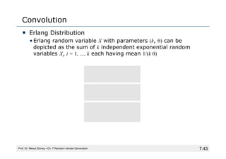
43.
7.43
Convolution
• Erlang Distribution
•Erlang random variable X with parameters (k, θ) can be
depicted as the sum of k independent exponential random
variables Xi, i = 1, …, k each having mean 1/(k θ)
Prof. Dr. Mesut Güneş ▪ Ch. 7 Random-Variate Generation
⎟
⎟
⎠
⎞
⎜
⎜
⎝
⎛
−
=
−
=
=
∏
∑
∑
=
=
=
k
i
i
k
i
i
k
i
i
R
k
R
k
X
X
1
1
1
ln
1
)
ln(
1
θ
θ
44.
7.44
Summary
• Principles ofrandom-variate generation via
• Inverse-transform technique
• Acceptance-rejection technique
• Special properties
• Important for generating continuous and discrete
distributions
Prof. Dr. Mesut Güneş ▪ Ch. 7 Random-Variate Generation
![7.4
Preparation
• It is assumed that a source of uniform [0,1] random
numbers exists.
• Linear Congruential Method (LCM)
• Random numbers R, R1, R2, … with
• PDF
• CDF
Prof. Dr. Mesut Güneş ▪ Ch. 7 Random-Variate Generation
⎩
⎨
⎧ ≤
≤
=
otherwise
0
1
0
1
)
(
x
x
fR
⎪
⎩
⎪
⎨
⎧
>
≤
≤
<
=
1
1
1
0
0
0
)
(
x
x
x
x
x
FR
0 1
f(x)
x
0 1
F(x)
x](https://image.slidesharecdn.com/randomvariategenerate-250805162232-52306d22/85/Random-variate-generate-for-simulation-pdf-4-320.jpg)
![7.8
Inverse-transform Technique: Example
• Exponential Distribution
• PDF
• CDF
• To generate X1, X2, X3 …
Prof. Dr. Mesut Güneş ▪ Ch. 7 Random-Variate Generation
x
e
x
f λ
λ −
=
)
(
x
e
x
F λ
−
−
=1
)
(
)
(
)
1
ln(
)
1
ln(
)
1
ln(
1
1
1
R
F
X
R
X
R
X
R
X
R
e
R
e
X
X
−
−
−
=
−
−
=
−
−
=
−
=
−
−
=
=
−
λ
λ
λ
λ
λ
• Simplification
• Since R and (1-R) are uniformly
distributed on [0,1]
λ
)
ln(R
X −
=](https://image.slidesharecdn.com/randomvariategenerate-250805162232-52306d22/85/Random-variate-generate-for-simulation-pdf-8-320.jpg)
![7.14
Inverse-transform Technique:
Uniform Distribution
• Random variable X uniformly distributed over [a, b]
Prof. Dr. Mesut Güneş ▪ Ch. 7 Random-Variate Generation
)
(
)
(
)
(
a
b
R
a
X
a
b
R
a
X
R
a
b
a
X
R
X
F
−
+
=
−
=
−
=
−
−
=](https://image.slidesharecdn.com/randomvariategenerate-250805162232-52306d22/85/Random-variate-generate-for-simulation-pdf-14-320.jpg)