Time series related presentation

1. Lecture 12:TIME SERIES DATA AND
THE PROBLEM OF
AUTOCORRELATION

2. Problem:
The regression models assume that the errors are independent (or uncorrelated)
random variables. This means that the different values of the response variable, Y,
can be related to the values of the predictor variables, the X’s, but not to one
another.
The usual interpretations of the results of a regression analysis depend heavily on
the assumption of independence.

3. Time Series Data Context:
With time series data, the assumption of independence rarely holds.
Consider the annual base price for a particular model of a new car. Can
you imagine the chaos that would exist if the new car prices from one
year to the next were indeed unrelated (independent) of one another?
In such a world, prices would be determined like numbers drawn from a
random number table. Knowledge of the price in one year would not
tell you anything about the price in the next year. In the real world, price
in the current year is related to (correlated with) the price in the
previous year, and maybe the price two years ago, and
so forth.
That is, the prices in different years are autocorrelated; they are not
independent.

4. Autocorrelation:

5. Autocorrelation is not all bad:
• From a forecasting perspective, autocorrelation is not all bad. If values
of a response, Y, in one time period are related to Y values in previous
time periods, then previous Y’s can be used to predict future Y’s.
• In a regression framework, autocorrelation is handled by “fixing up”
the standard regression model. To accommodate autocorrelation,
sometimes it is necessary to change the mix of predictor variables
and/or the form of the regression function.
• More typically, however, autocorrelation is handled by changing the
nature of the error term.

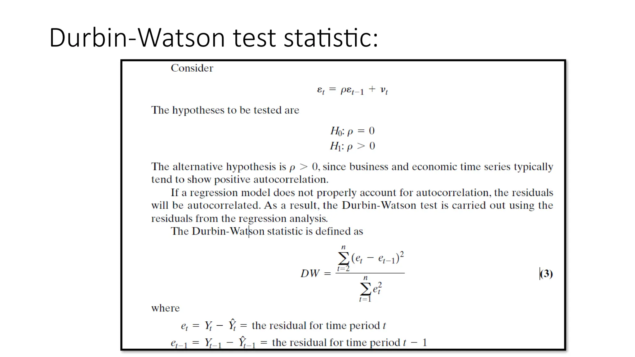
6. First-order serial correlation:
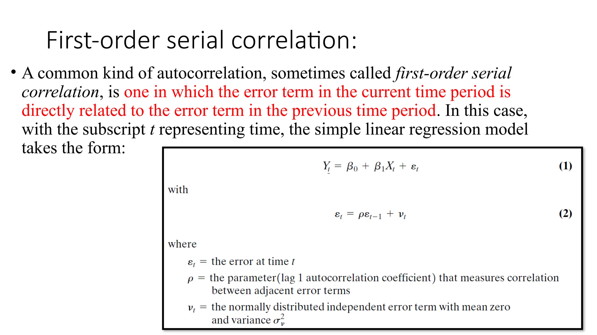
• A common kind of autocorrelation, sometimes called first-order serial
correlation, is one in which the error term in the current time period is
directly related to the error term in the previous time period. In this case,
with the subscript t representing time, the simple linear regression model
takes the form:

7. Strength of serial correlation:

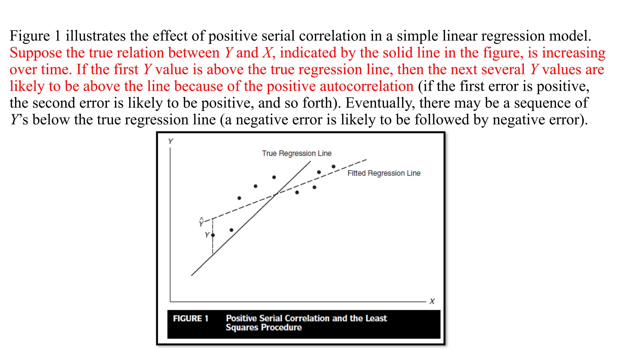
8. Figure 1 illustrates the effect of positive serial correlation in a simple linear regression model.
Suppose the true relation between Y and X, indicated by the solid line in the figure, is increasing
over time. If the first Y value is above the true regression line, then the next several Y values are
likely to be above the line because of the positive autocorrelation (if the first error is positive,
the second error is likely to be positive, and so forth). Eventually, there may be a sequence of
Y’s below the true regression line (a negative error is likely to be followed by negative error).

9. Problems with the inference:
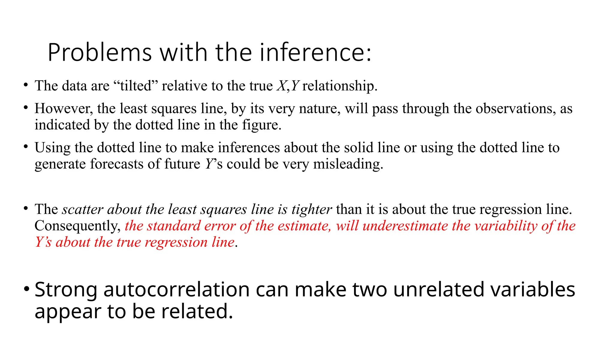
• The data are “tilted” relative to the true X,Y relationship.
• However, the least squares line, by its very nature, will pass through the observations, as
indicated by the dotted line in the figure.
• Using the dotted line to make inferences about the solid line or using the dotted line to
generate forecasts of future Y’s could be very misleading.
• The scatter about the least squares line is tighter than it is about the true regression line.
Consequently, the standard error of the estimate, will underestimate the variability of the
Y’s about the true regression line.
• Strong autocorrelation can make two unrelated variables
appear to be related.

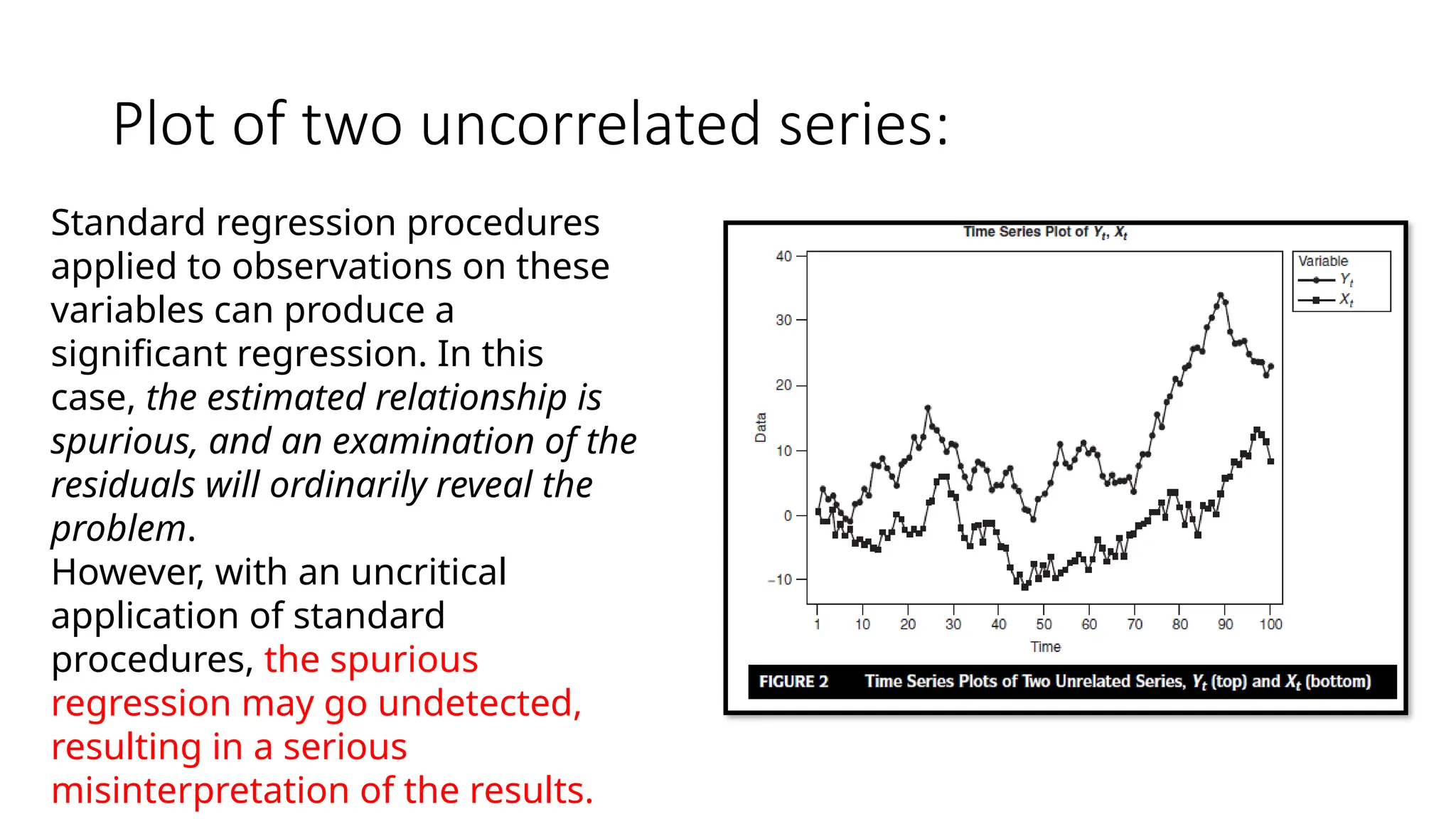
10. Plot of two uncorrelated series:
Standard regression procedures
applied to observations on these
variables can produce a
significant regression. In this
case, the estimated relationship is
spurious, and an examination of the
residuals will ordinarily reveal the
problem.
However, with an uncritical
application of standard
procedures, the spurious
regression may go undetected,
resulting in a serious
misinterpretation of the results.

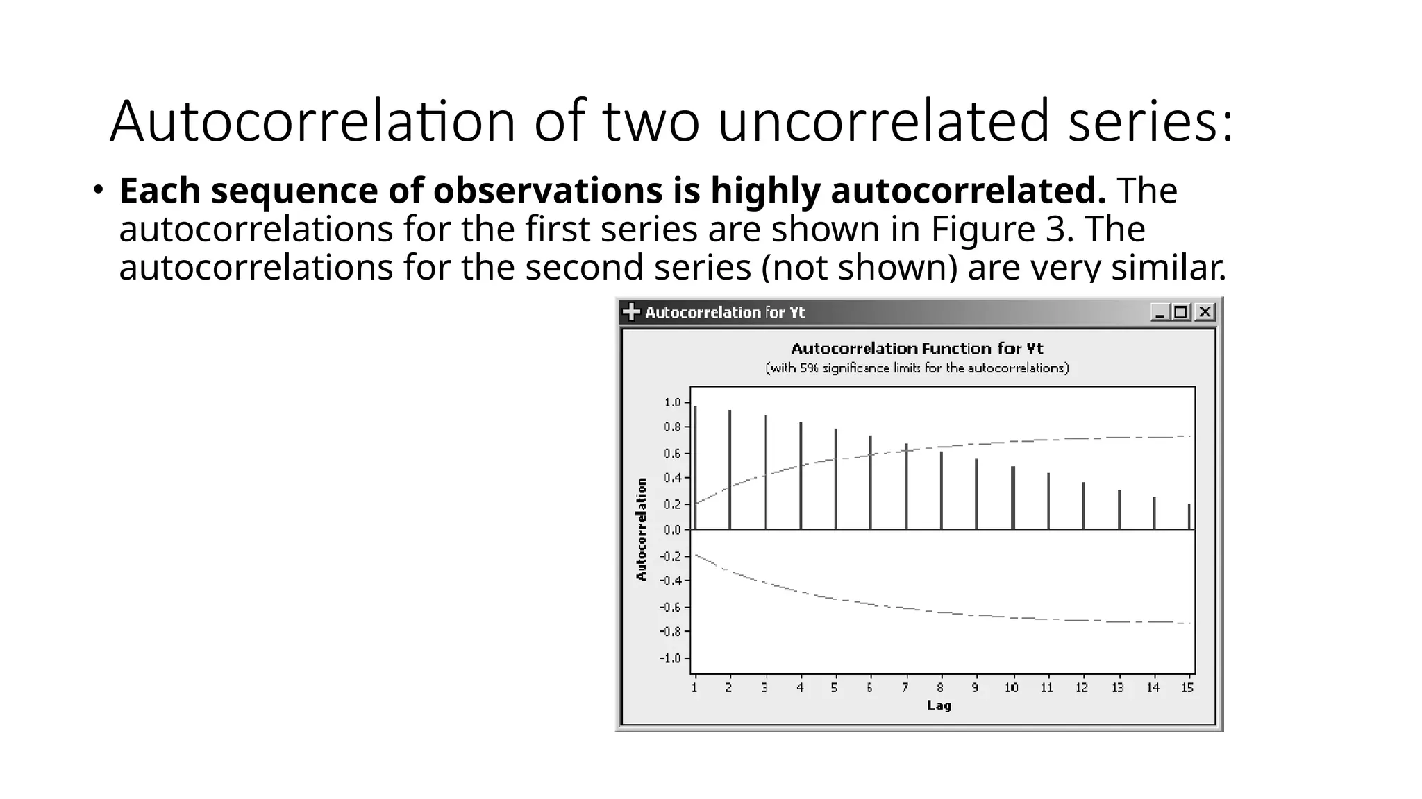
11. Autocorrelation of two uncorrelated series:
• Each sequence of observations is highly autocorrelated. The
autocorrelations for the first series are shown in Figure 3. The
autocorrelations for the second series (not shown) are very similar.

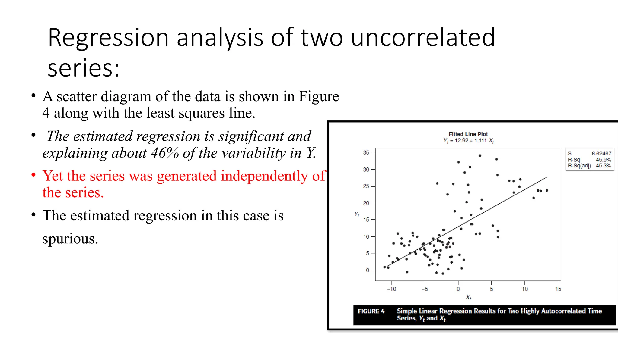
12. Regression analysis of two uncorrelated
series:
• A scatter diagram of the data is shown in Figure
4 along with the least squares line.
• The estimated regression is significant and
explaining about 46% of the variability in Y.
• Yet the series was generated independently of
the series.
• The estimated regression in this case is
spurious.

13. Where is the fault?
• The fault is not with the least squares procedure. The fault lies in applying
the standard regression model in a situation that does not correspond to the
usual regression assumptions. The technical problems that arise include the
following:
1. The standard error of the estimate can seriously underestimate the variability
of the error terms.
2. The usual inferences based on the t and F statistics are no longer strictly
applicable.
3. The standard errors of the regression coefficients underestimate the
variability of the estimated regression coefficients. Spurious regressions can
result.

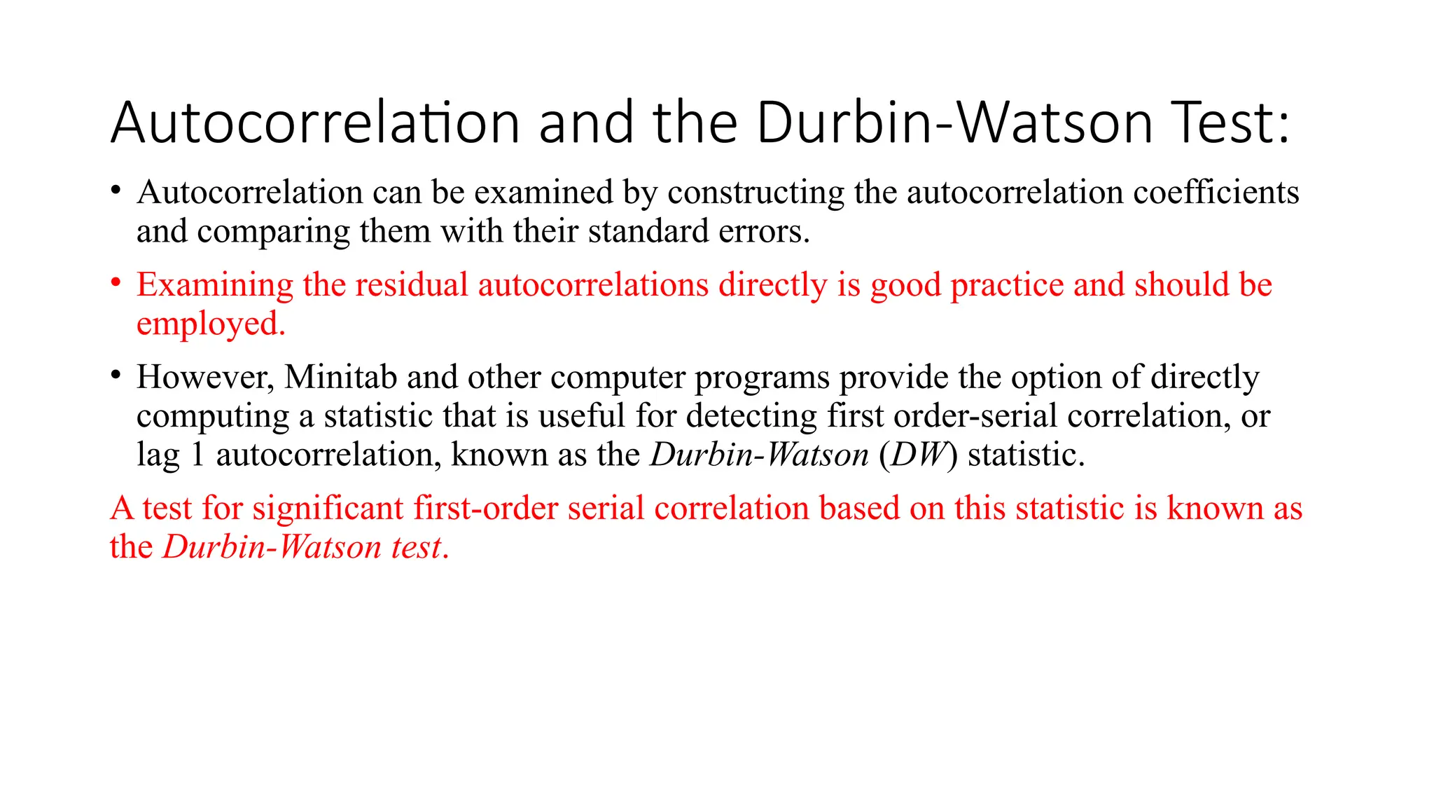
14. Autocorrelation and the Durbin-Watson Test:
• Autocorrelation can be examined by constructing the autocorrelation coefficients
and comparing them with their standard errors.
• Examining the residual autocorrelations directly is good practice and should be
employed.
• However, Minitab and other computer programs provide the option of directly
computing a statistic that is useful for detecting first order-serial correlation, or
lag 1 autocorrelation, known as the Durbin-Watson (DW) statistic.
A test for significant first-order serial correlation based on this statistic is known as
the Durbin-Watson test.

15. Durbin-Watson test statistic:

16. Decision rules for Durbin-Watson test:

17. Durbin-Watson Table
(

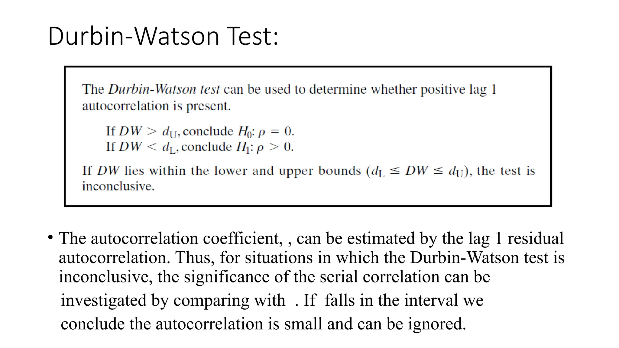
18. Durbin-Watson Test:
• The autocorrelation coefficient, , can be estimated by the lag 1 residual
autocorrelation. Thus, for situations in which the Durbin-Watson test is
inconclusive, the significance of the serial correlation can be
investigated by comparing with . If falls in the interval we
conclude the autocorrelation is small and can be ignored.

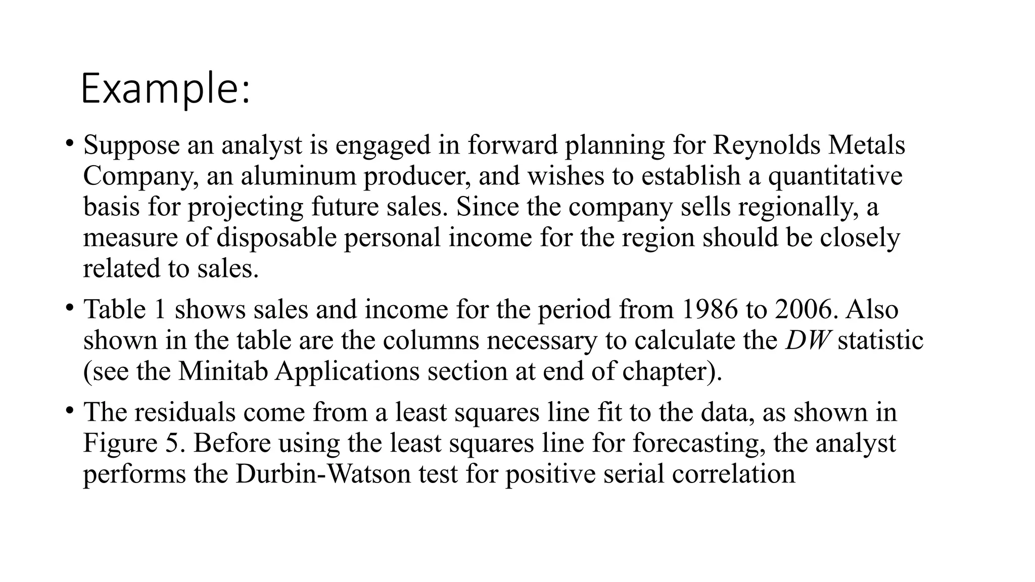
19. Example:
• Suppose an analyst is engaged in forward planning for Reynolds Metals
Company, an aluminum producer, and wishes to establish a quantitative
basis for projecting future sales. Since the company sells regionally, a
measure of disposable personal income for the region should be closely
related to sales.
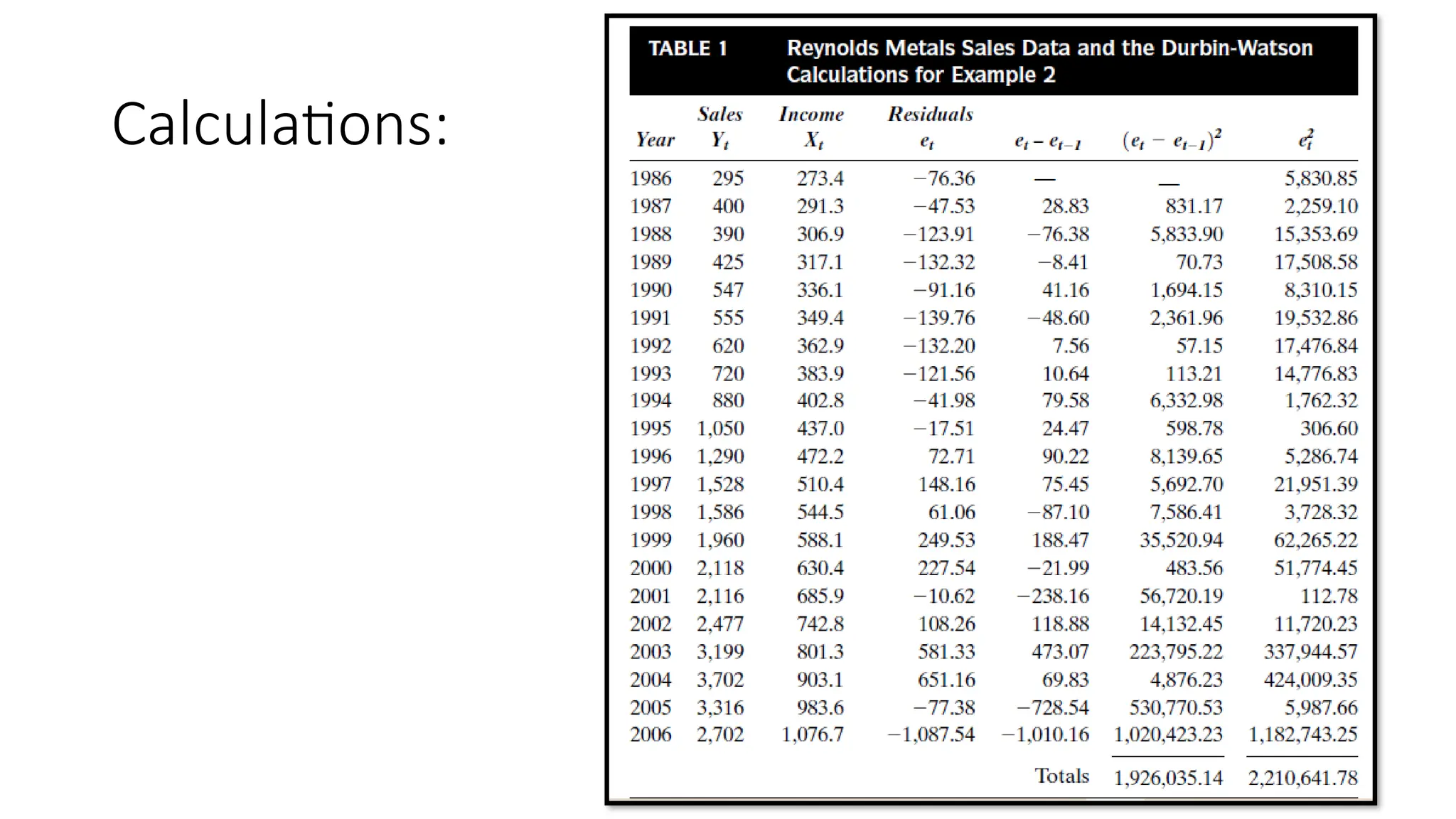
• Table 1 shows sales and income for the period from 1986 to 2006. Also
shown in the table are the columns necessary to calculate the DW statistic
(see the Minitab Applications section at end of chapter).
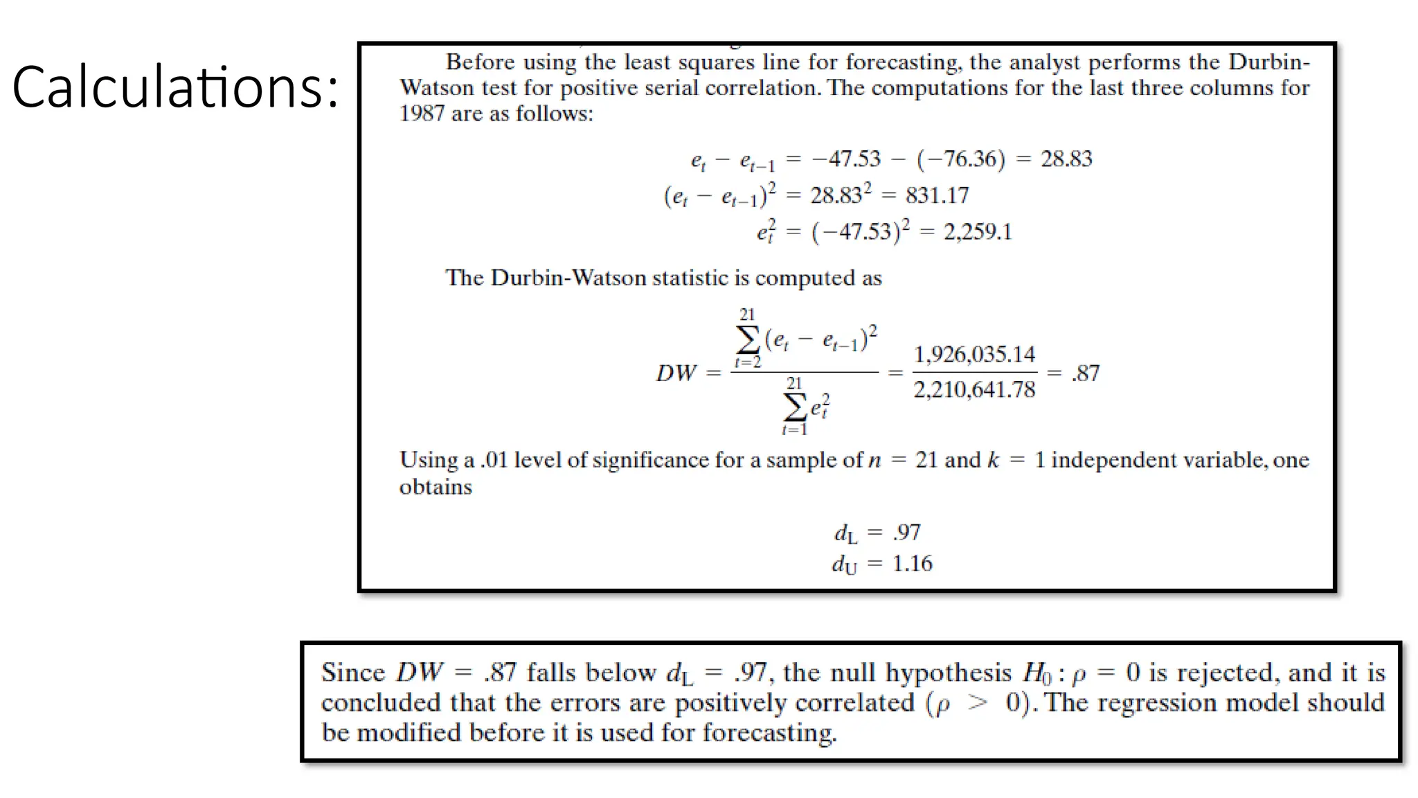
• The residuals come from a least squares line fit to the data, as shown in
Figure 5. Before using the least squares line for forecasting, the analyst
performs the Durbin-Watson test for positive serial correlation

20. Regression Equation:

21. Calculations:

22. Calculations:

23. Solution to autocorrelation problems:
• The solution to the problem of autocorrelation begins with an
evaluation of the model specification.
• Is the functional form correct?
• Were any important variables omitted?
• Are there effects that might have some pattern over time that could
have introduced autocorrelation into the errors?

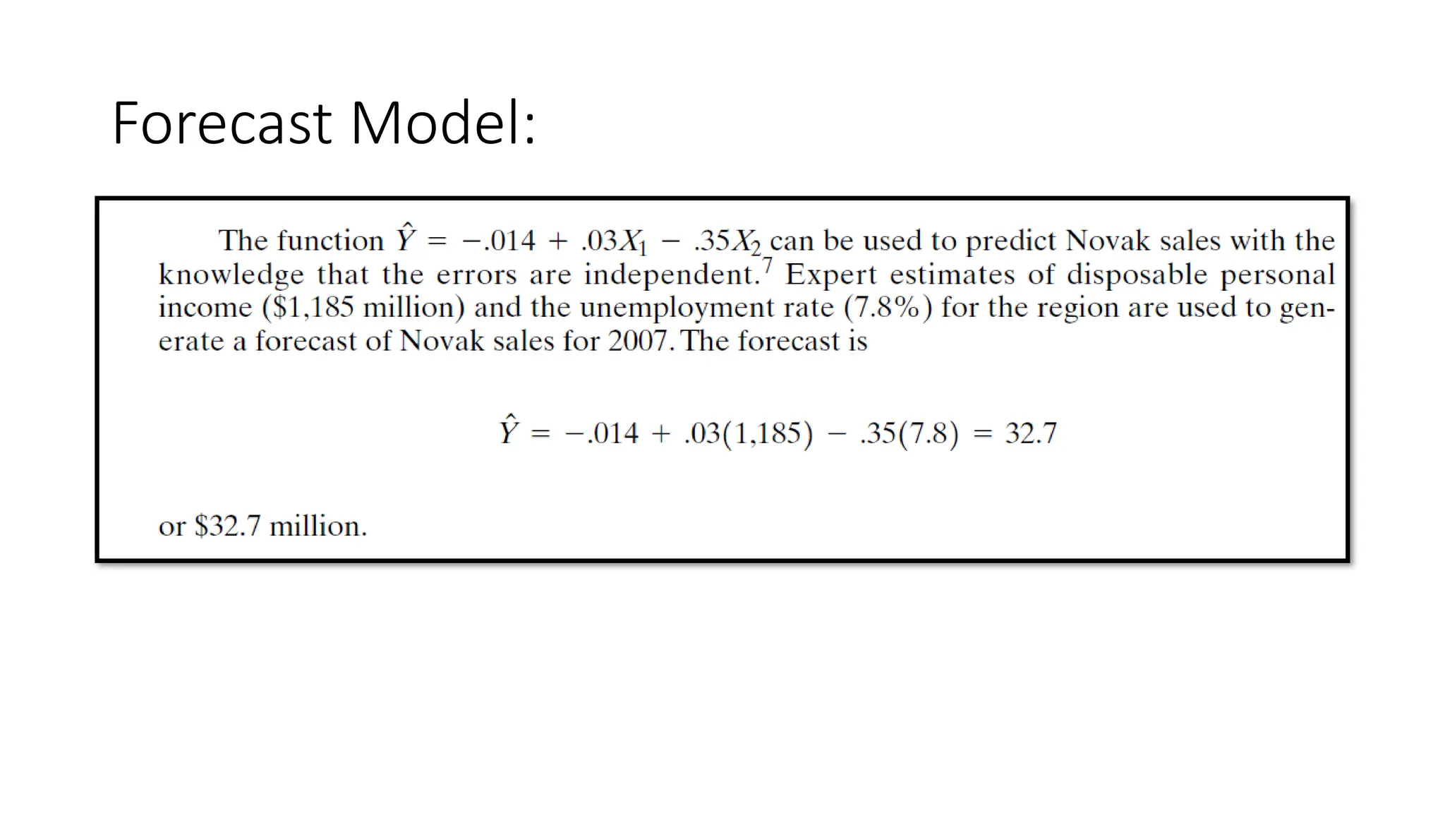
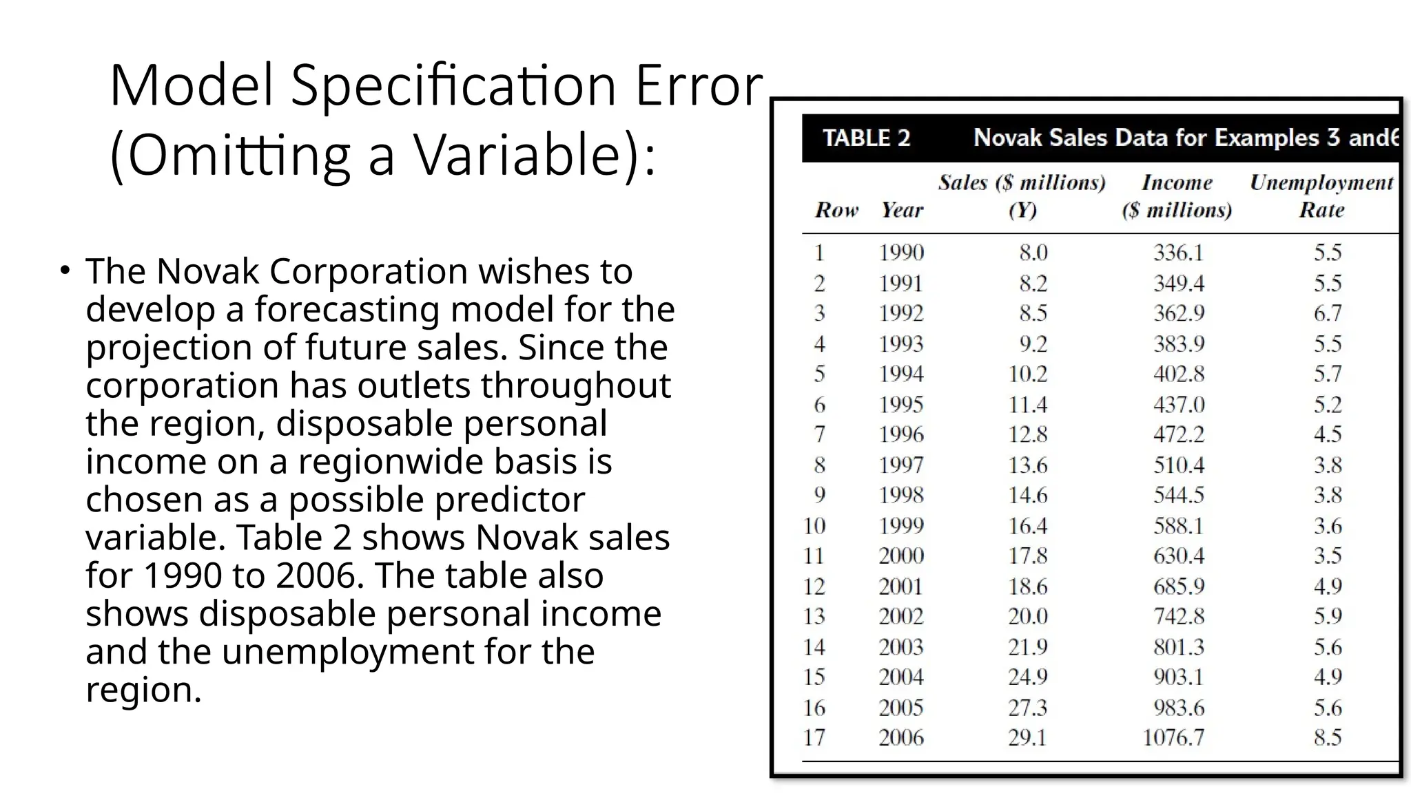
24. Model Specification Error
(Omitting a Variable):
• The Novak Corporation wishes to
develop a forecasting model for the
projection of future sales. Since the
corporation has outlets throughout
the region, disposable personal
income on a regionwide basis is
chosen as a possible predictor
variable. Table 2 shows Novak sales
for 1990 to 2006. The table also
shows disposable personal income
and the unemployment for the
region.

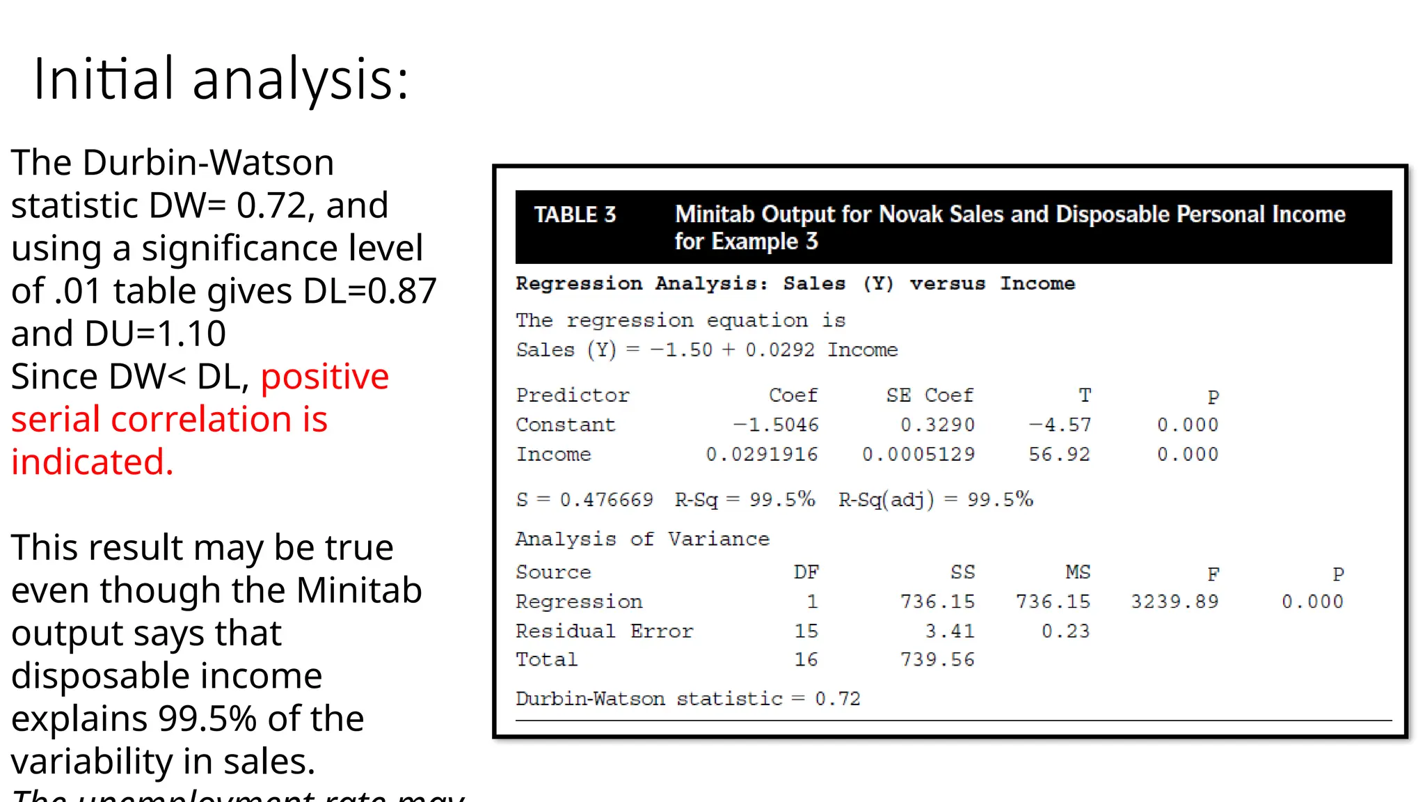
25. Initial analysis:
The Durbin-Watson
statistic DW= 0.72, and
using a significance level
of .01 table gives DL=0.87
and DU=1.10
Since DW< DL, positive
serial correlation is
indicated.
This result may be true
even though the Minitab
output says that
disposable income
explains 99.5% of the
variability in sales.

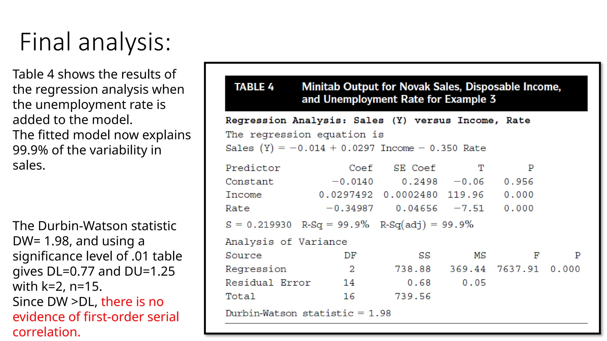
26. Final analysis:
Table 4 shows the results of
the regression analysis when
the unemployment rate is
added to the model.
The fitted model now explains
99.9% of the variability in
sales.
The Durbin-Watson statistic
DW= 1.98, and using a
significance level of .01 table
gives DL=0.77 and DU=1.25
with k=2, n=15.
Since DW >DL, there is no
evidence of first-order serial
correlation.

27. Forecast Model:

28. Regression with Differences:

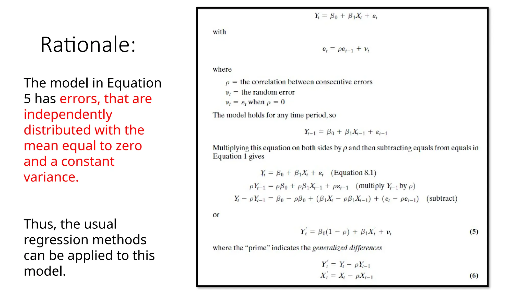
29. Rationale:
The model in Equation
5 has errors, that are
independently
distributed with the
mean equal to zero
and a constant
variance.
Thus, the usual
regression methods
can be applied to this
model.

30. Regression with First Differences:

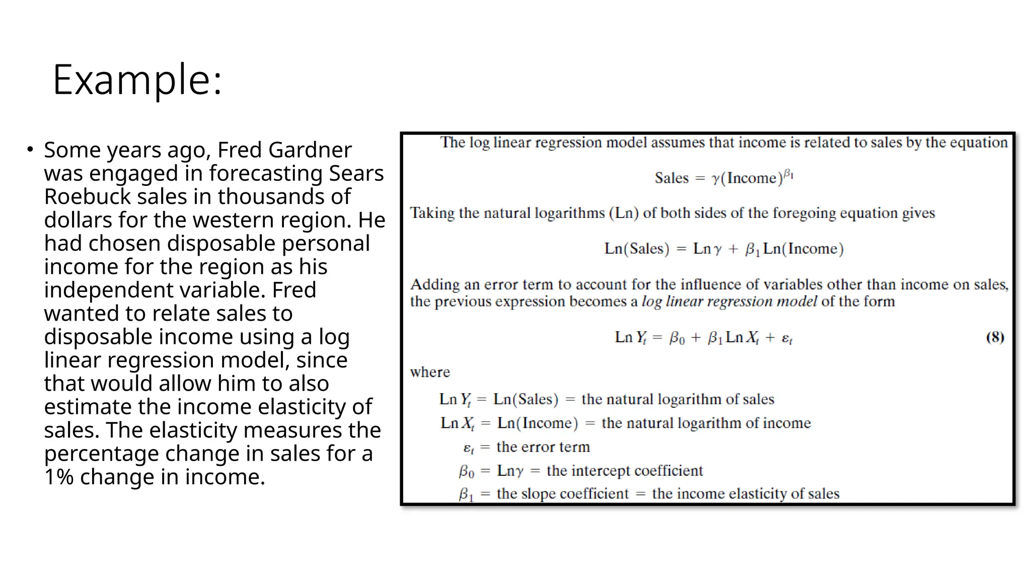
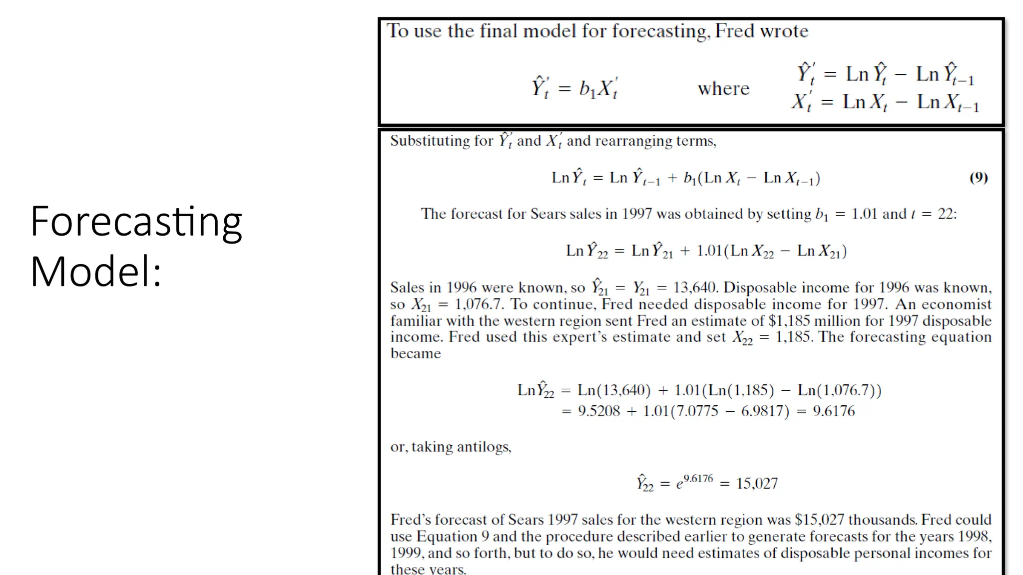
31. Example:
• Some years ago, Fred Gardner
was engaged in forecasting Sears
Roebuck sales in thousands of
dollars for the western region. He
had chosen disposable personal
income for the region as his
independent variable. Fred
wanted to relate sales to
disposable income using a log
linear regression model, since
that would allow him to also
estimate the income elasticity of
sales. The elasticity measures the
percentage change in sales for a
1% change in income.

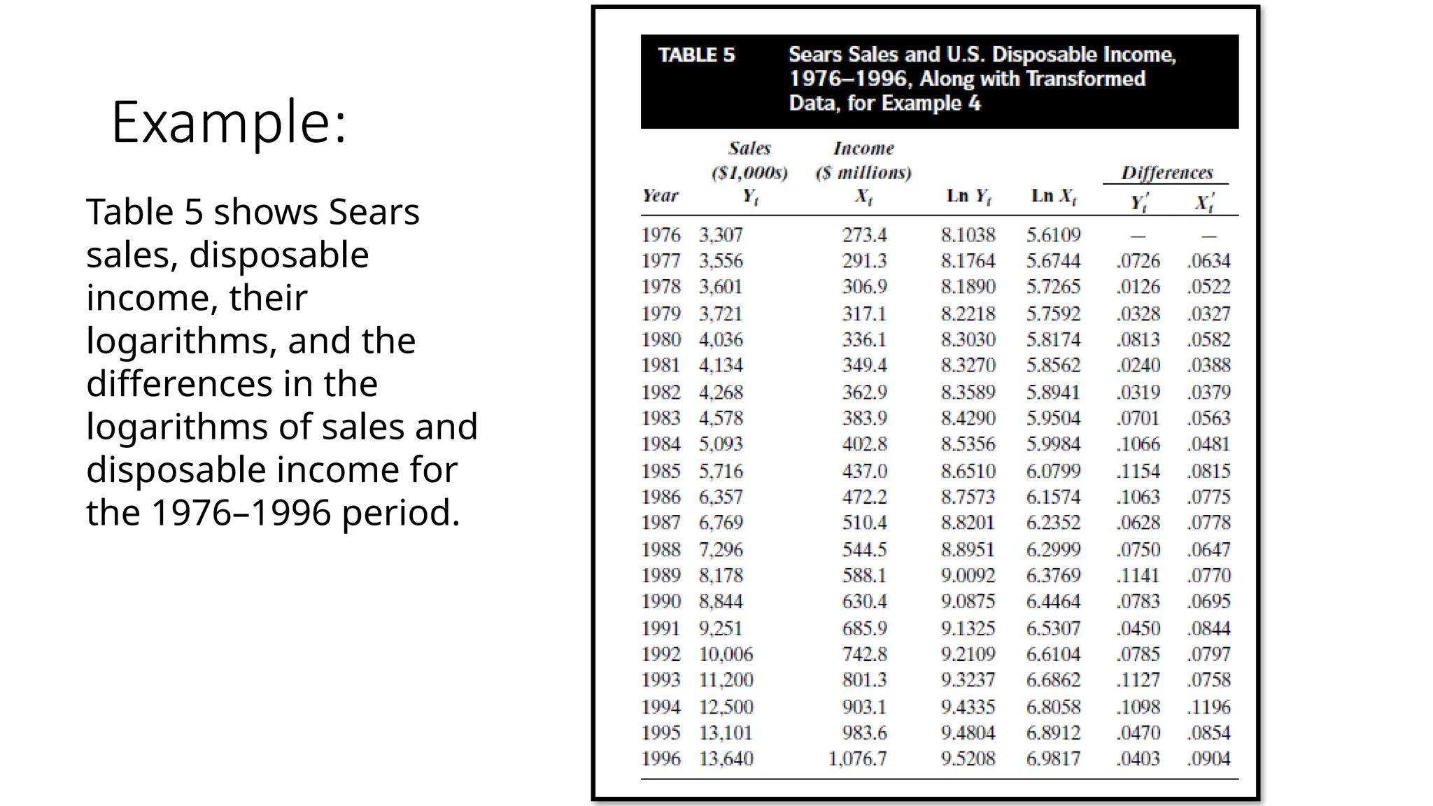
32. Example:
Table 5 shows Sears
sales, disposable
income, their
logarithms, and the
differences in the
logarithms of sales and
disposable income for
the 1976–1996 period.

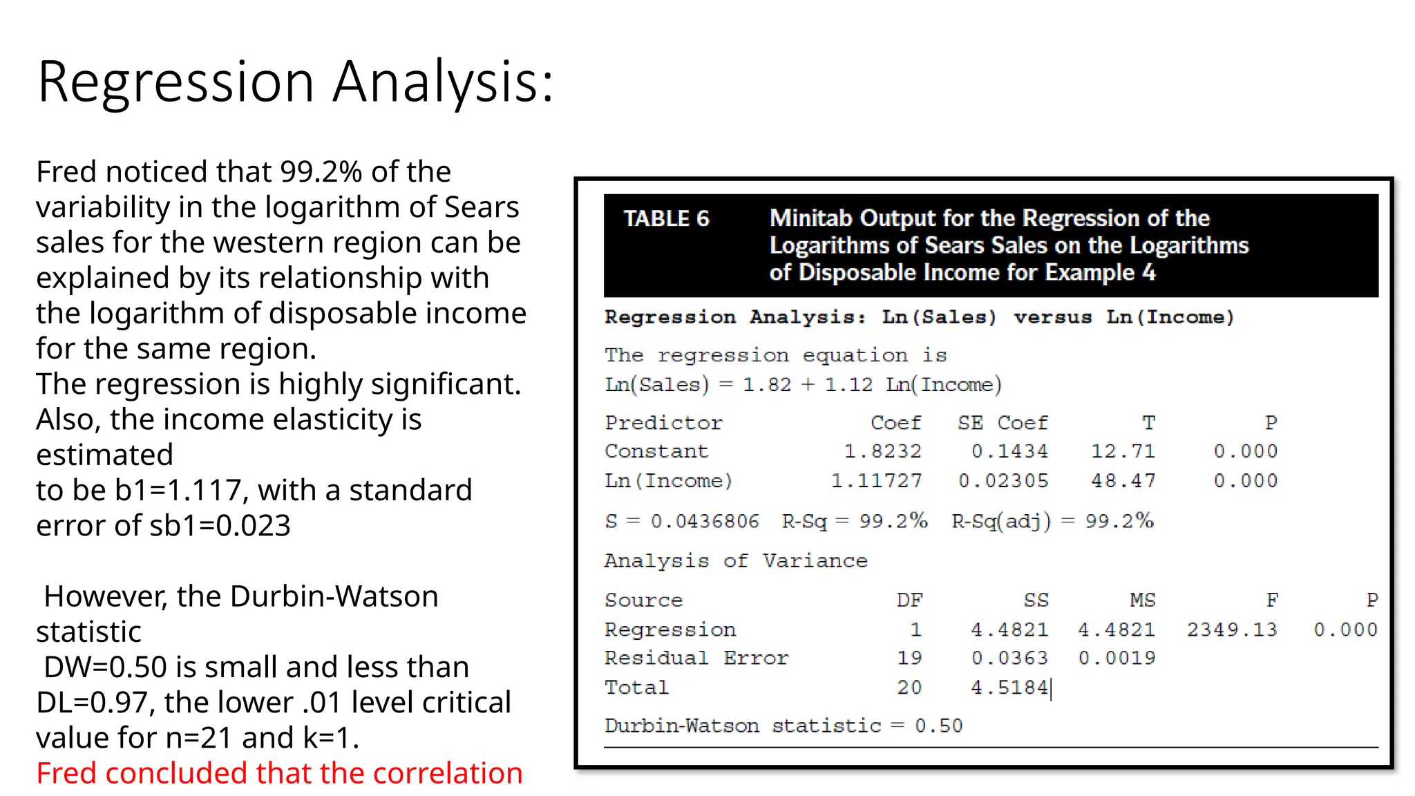
33. Regression Analysis:
Fred noticed that 99.2% of the
variability in the logarithm of Sears
sales for the western region can be
explained by its relationship with
the logarithm of disposable income
for the same region.
The regression is highly significant.
Also, the income elasticity is
estimated
to be b1=1.117, with a standard
error of sb1=0.023
However, the Durbin-Watson
statistic
DW=0.50 is small and less than
DL=0.97, the lower .01 level critical
value for n=21 and k=1.
Fred concluded that the correlation

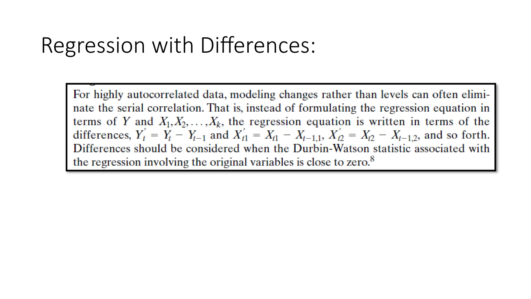
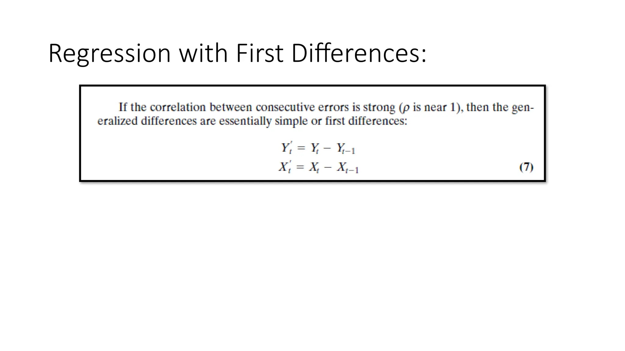
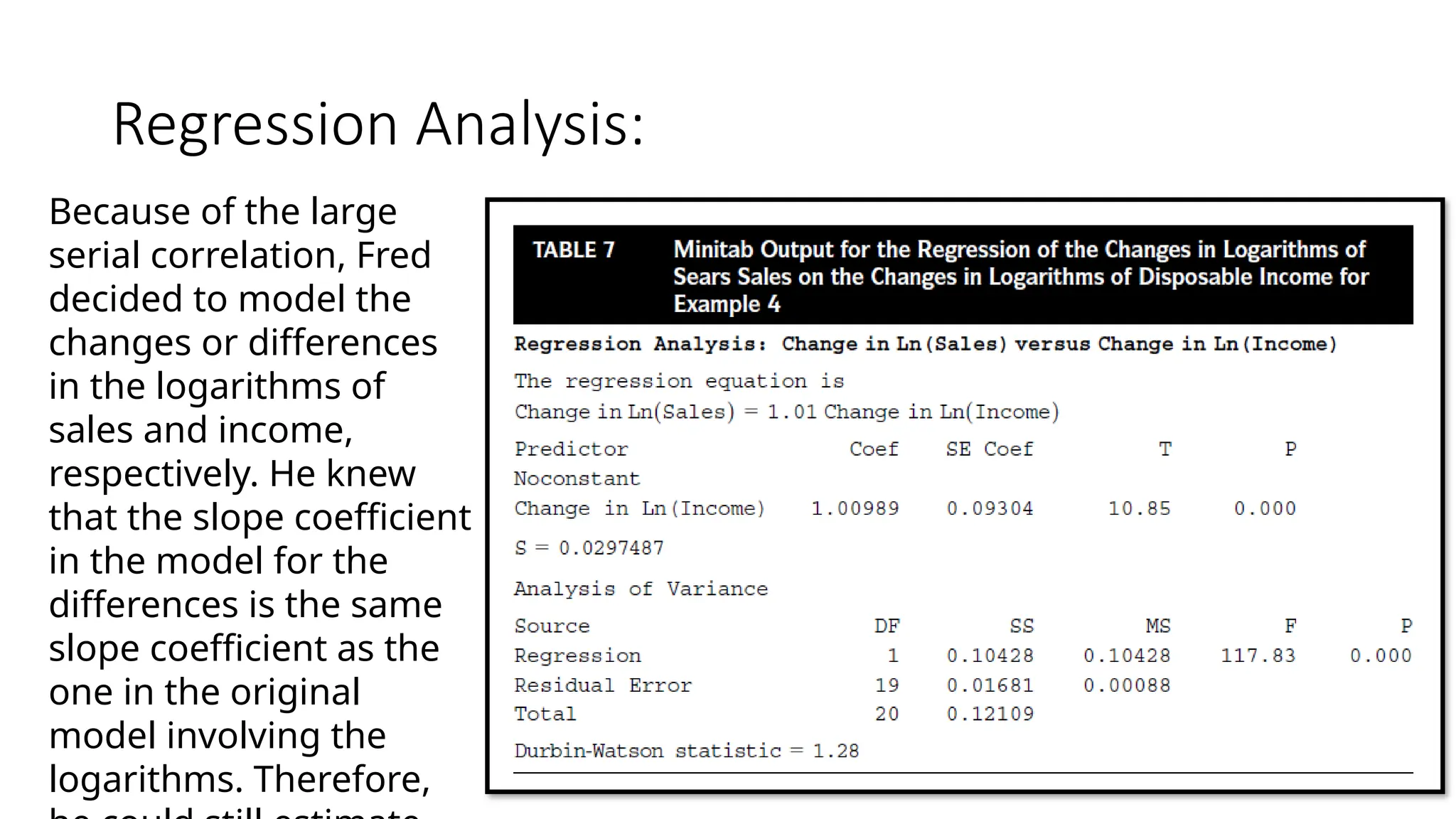
34. Regression Analysis:
Because of the large
serial correlation, Fred
decided to model the
changes or differences
in the logarithms of
sales and income,
respectively. He knew
that the slope coefficient
in the model for the
differences is the same
slope coefficient as the
one in the original
model involving the
logarithms. Therefore,

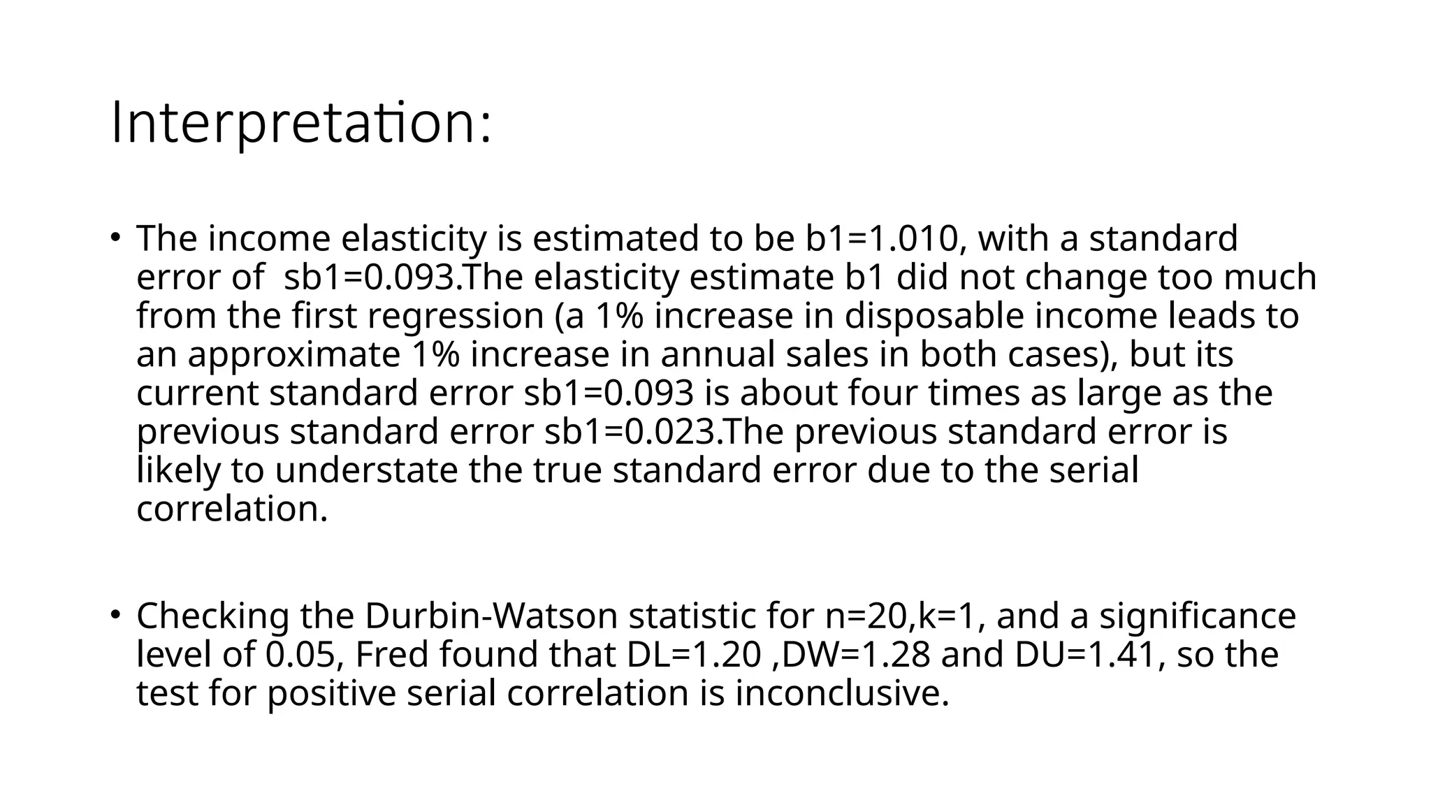
35. Interpretation:
• The income elasticity is estimated to be b1=1.010, with a standard
error of sb1=0.093.The elasticity estimate b1 did not change too much
from the first regression (a 1% increase in disposable income leads to
an approximate 1% increase in annual sales in both cases), but its
current standard error sb1=0.093 is about four times as large as the
previous standard error sb1=0.023.The previous standard error is
likely to understate the true standard error due to the serial
correlation.
• Checking the Durbin-Watson statistic for n=20,k=1, and a significance
level of 0.05, Fred found that DL=1.20 ,DW=1.28 and DU=1.41, so the
test for positive serial correlation is inconclusive.

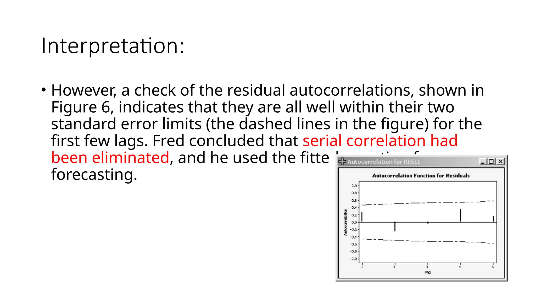
36. Interpretation:
• However, a check of the residual autocorrelations, shown in
Figure 6, indicates that they are all well within their two
standard error limits (the dashed lines in the figure) for the
first few lags. Fred concluded that serial correlation had
been eliminated, and he used the fitted equation for
forecasting.

37. Forecasting
Model: