2. March 26, 2010
Peru: Staff Report for the 2010 Article IV Consultation
Selected Issues
Prepared by the Western Hemisphere Department
(In collaboration with other departments)
Contents
I. Performance of Alternative Fiscal Rules: An Application to Peru ................................................... 2
II. What to Expect when you are Expecting...Large Capital Inflows? Lessons from Cross-
Country Experiences ................................................................................................................. 22
III. Peru: Drivers of De-Dollarization .................................................................................................. 35
IV. Potential Growth and Output Gap in Peru .................................................................................... 57
V. Progress in Strengthening Peru’s Prudential Framework ............................................................ 68
Selected Issues - Staff Report Article IV 2010 Consultation – Peru
3. Performance of Alternative Fiscal Rules:
An Application to Peru
This chapter assesses the performance of alternative fiscal rules in supporting medium-term
fiscal policy objectives. Three main conclusions emerge from the analysis. First, there is no
dominance of one rule to the others but rather each one involves trade-offs in terms of
sustainability, cyclicality, volatility of main fiscal variable, and different degrees of implementation
challenges. Second, the selection of a particular rule should be based on its performance relative
to a prioritized set of fiscal policy objectives. In the case of Peru, the analysis suggests that a
structural approach could result in important gains in terms of limiting pro-cyclical effects.
However, a formal structural balance rule can be demanding in terms of economic and
institutional prerequisites, entailing lengthy preparatory steps. Third, the current Fiscal
Responsibility and Transparency Law (FRTL) has been critical for debt reduction in Peru, with
embedded flexibility to adapt to evolving objectives. A change in FRTL parameters can replicate
some of the features of a structural balance rule, while preserving debt limit objectives.
I. Background
1. The Peruvian authorities have shown a strong commitment to prudent fiscal policy. In
1999, the first version of the Fiscal Responsibility and Transparency Law (FRTL) was introduced,
representing a structural change in fiscal strategy in Peru (Box). While the FRTL was instrumental
for fiscal consolidation, controlling spending has been challenging and caps frequently proved to
be difficult to enforce, particularly at the sub-national level. Overall, against a backdrop of strong
growth and high commodity prices, fiscal policy has been slightly counter-cyclical.
2. The current global financial crisis has strained national fiscal rules over the world,
with fiscal rules in many countries being modified, including in Peru.2 Thanks to large
saving accumulated in recent years, Peru was able to implement a significant fiscal stimulus that
entailed a positive fiscal impulse of about 21 e2 percent of GDP in 2009—a 14 percent increase in
real general government primary spending, far beyond the cap established in the FRTL. Also, the
FRTL was modified to increase the 1 percent of GDP deficit limit to 2 percent in 2009í2010.In
2010, with increasing evidence of a self-sustained rebound, fiscal policy is moving towards a
neutral fiscal stance, returning to the FRTL debt limit in 2011.
1
Prepared by I. Rial (FAD).
2
For a detailed assessment of the international experience see “Fiscal Rules: Anchoring Expectations for
Sustainable Public Finances” IMF Policy Paper, November.
Selected Issues - Staff Report Article IV 2010 Consultation – Peru 2
4. 3. While recent efforts to strengthen the fiscal framework have been significant,
challenges remain to formalize a more explicit medium-term orientation of fiscal policy.
Main challenges comprise the adoption and implementation of a fiscal rule that could help
maintain public finances on a sustainable path, smooth output fluctuations, and create a
budgetary cushion against adverse shocks and long-term fiscal pressures.
4. This chapter assesses the performance of alternative fiscal rules in supporting
medium-term fiscal policy objectives. Three principal conclusions emerge from the analysis.
First, none of the rules examined clearly dominates the others. Rather, each one involves trade-
offs in terms of sustainability, cyclicality, volatility of main fiscal variable, and different degrees of
implementation challenges. Second, the selection of the appropriate rule should be based on its
performance relative to a prioritized set of fiscal policy objectives. In the case of Peru, the
analysis suggests that a structural rule could have substantial gains while risks remain contained.
However, a structural rule can be demanding in terms of economic and institutional prerequisites,
entailing lengthy preparatory steps. Third, the current FRTL has proven to be flexible and a
change in parameters can replicate the results of a structural rule, while preserving debt limit
objectives.
II. Main Results
5. This section assesses the fiscal implications of alternative fiscal rules under a variety
of scenarios. To illustrate how fiscal variables behave under alternative rules, we present two
sets of simulations. First, we simulate how fiscal variables would have behaved if these rules had
EHHQ LQ SODFH GXULQJ í8—i.e., a deterministic backwards looking exercise. Second, we
discuss the results of the implementation of the same rules for the next fLYH HDUV í
5. under both deterministic and stochastic scenarios.
6. Four fiscal rules are considered in the simulations: (i) a basic balance budget rule, which
targets a zero nominal overall balance; (ii) a expenditure rule, which caps real primary
expenditures increase to 5.5 percent a year; (iii) a structural balance rule, which targets a zero
primary balance adjusted to account for medium-term output and commodity prices levels; and
(iv) the Peruvian FRTL rule, which allows for an overall fiscal deficit of up to 1.0 percent of GDP in
“bad” times, while capping the increase in real expenditures to 3.0 percent in “good” times. 3,4
7. Assessing the performance of alternative rules entails trade-offs between various
policy objectives and medium-term fiscal risks. Fiscal rules can serve different policy
3
Bad times are defined as those years where real GDP growths below its potential rate. Good times are
defined accordingly.
4
For simplicity purposes, the “theoretical” Peruvian rule is a stylized version of the “real” rule.
Selected Issues - Staff Report Article IV 2010 Consultation - Peru 3
6. Box. 1 Peruvian Fiscal Rule
Legal status of the rule. As part of the effort to alleviate medium-term PFM shortcomings, the “Ley de
Responsabilidad y Transparencia Fiscal” (FRTL) was enacted in December 1999 as a permanent
institutional device to promote fiscal discipline in a credible, predictable, and transparent manner. In
2003 the Fiscal Management Responsibility Act was introduced with a clear objective of debt
consolidation.
Rationale for the fiscal rule. The FRTL included a combination of a deficit target and real current
expenditure ceiling for the nonfinancial public sector and general government respectively, as well as
debt ceilings for subnational governments. The main features of the Peruvian FRL can be summarized
as follows:
x It contains procedural and transparency provisions; particularly, the government must prepare the
Multi-Annual Macroeconomic Framework (Marco Macroeconómico Multianual) containing three-year
macroeconomic projections of revenue, expenditure, public investment, and public debt.
x Numerical fiscal targets are embedded in the law (see table below).
x Institutional coverage is broad, covering the nonfinancial public sector (although not for all targets).
x Sanctions are only institutional.
x Escape clauses allow deviations from numerical targets during periods of low growth.
x Cyclical considerations are taken into account by establishing fiscal stabilization funds to mitigate
cyclical variations.
Historical compliance with the rule. The numerical targets embedded in the law were changed over
time, such as in 2003, 2007 and 2009. The following table summarizes the main changes introduced to
the FRTL.
E d Z d Zd
D E Z
E W ^ 'W
' '
'
E W ^ 'W
' '
'
^ D D Z s W
Z W
E
Response to the global financial crisis. The impact of the recent global financial crisis has been
significant, which called for countercyclical monetary and fiscal policies. Escape clauses in the law were
not applicable for this particular shock. However, the FRTL includes an exceptional escape clause that
allows for a temporary relaxation of the targets with Congressional approval. The relaxation of the FRTL
targets was approved in May 2009 to allow a deficit of 2 percent of GDP and to undertake a
countercyclical fiscal policy response.
Selected Issues - Staff Report Article IV 2010 Consultation - Peru 4
7. objectives, such as: promote fiscal sustainability, provide cyclical flexibility (the ability to respond
to shocks), promote economic stabilization, contain the size of the government, support
intergenerational equity, etc. Each type of fiscal rule has different properties relative to key policy
objectives. Furthermore, priorities may change over time once gains from past policies are
achieved, which may justify a change of the fiscal rule in place.
8. We use summary indicators to compare the performance of alternative rules to
achieve different policy objectives. Rules are compared with regards to its ability to: (i) ensure
a sustainable debt path (sustainability); (ii) ensure a neutral stance relative to the cycle
(cyclicality);5 (iii) help deliver the required adjustment without requiring a significant fiscal effort
that may not be politically feasible; (iv) minimize volatility of main fiscal variables; and (v) allow for
the accumulation of fiscal buffers in “good” times. To obtain a more realistic assessment of the
merits of alternative fiscal rules in the medium-term we introduce a stochastic approach to
discuss the appropriate level of risks that the authorities might be willing to take.
$SSOLFDWLRQ RI $OWHUQDWLYH 5XOHV IRU í8
9. As a deterministic EDFNZDUG ORRNLQJ H[HUFLVH IRU WKH SHULRG í ZH VLPXODWH
the fiscal path under the four alternative rules, assuming that they were binding and met
every year. Table 1 and Figure 1 present the main results.
. Key conclusions emerge from this exercise:
x All proposed rules show similar results in terms of fiscal sustainability. Debt ratio remains
around 40 percent of GDP in average for the period, similar to actual levels.
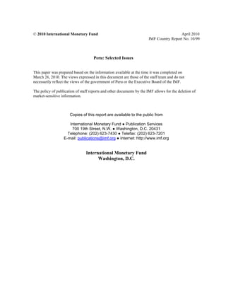
x Not surprisingly, the structural balance rule and, to a lesser extent, the actual fiscal data
exhibit a more neutral stance; while the balance budget rule is procyclical and the
expenditure rule countercyclical. The Peruvian theoretical rule gives similar results to the
expenditure rule for this period.
x Discrepancies between the results of the Peruvian theoretical rule and actual fiscal data derive
from temporary deviations of actual policy from the theoretical rule. As shown in Figure 1, in
2008 actual fiscal data shows a procyclical stance (real expenditures increased significantly
over the cap in the context of a highly positive output gap), while under the theoretical rule
fiscal stance would have been counter cyclical.
5
To measure the procyclical bent in a fiscal rule we calculated the cumulative pro-cyclical impulses over the
reference period (as proposed by Debrun, et altri IMF WP/08/87). That means improvements in the primary
balance during bad times, and deteriorations of the primary balance in good times (in percent of GDP). The
higher the indicator, the more procyclical the rule is.
Selected Issues - Staff Report Article IV 2010 Consultation - Peru 5
8. x The structural balance rule requires the lowest fiscal effort, measured as the minimum real
change in primary expenditures in one year. The Peruvian theoretical rule and the balance
budget rule are the ones requiring the larger fiscal effort.
x The expenditure rule shows the lowest volatility, measured by the standard deviation of real
changes of primary expenditures. Under the balance budget rule, shocks to GDP affect tax
revenues and lead to a corresponding adjustment in expenditures. Under the structural rule,
shocks to GDP would also affect the output gap offsetting the required adjustment in
expenditure, thus resulting in a smoother expenditure pattern. The Peruvian theoretical rule
shows very similar results to the structural balance rule in terms of spending fluctuations
during this period.
x The Peruvian theoretical rule allows for the highest accumulation of fiscal surpluses in “good
years, followed by the structural balance rule. These two rules promote the building up of
fiscal buffers that could be used in less favorable years. The balance budget rule does not
allow for accumulation of fiscal surpluses by construction. Under the expenditure rule, while
fiscal performance improves in good years, it is not enough to generate an overall surplus
during this period.
Table 1. Comparative Performance of Alternative Fiscal Rules, 1998í2008.
Actual Alternative Rules applied over the period
data
1998-2008 Balance Structural Peruvian
Exp. Rule
Budget 5.5% real Balance theoretical
Indicator (in % of GDP, unless otherwise stated) Rule change Rule Rule
A. Sustainability
Average gross debt in the period 39.7 38.7 42.7 39.6 38.7
B. Cyclicality
Cummulative Fiscal Impulse over the period (+) procyclical; (-) countercyclical 1/ -1.1 4.7 -2.6 0.0 -2.9
C. Fiscal effort
Minimum change in primary expenditure in one year (real change) -3.7 -6.9 5.5 -1.2 -6.5
D. Volatility
Standard deviation of real primary expenditures (real change) 5.9 8.7 0.0 4.6 4.7
E. Accumulation of overall surpluses in good years
(good year GDP growth than potential) 7.0 0.0 0.0 1.0 10.2
Source: Staff estimations.
1/ Cumulative pro-cyclical impulses over the reference period (as proposed by 'HEUXQ HW DOWUL ,0) :3 ).
That means improvements in the primary balance during bad times, and deteriorations of the primary balance in good times (in % GDP).
Selected Issues - Staff Report Article IV 2010 Consultation - Peru 6
9. Figure 1. Output Gap, FKDQJH LQ 2XWSXW *DS DQG )LVFDO ,PSXOVH í8
Output gap
% GDP
4.0
2.0
0.0
-2.0
-4.0
1999 2000 2001 2002 2003 2004 2005 2006 2007 2008
Fiscal Impulse and change in Output Gap
Actual fiscal stance
3.0
2.0
1.0
0.0
-1.0
-2.0
-3.0
1999 2000 2001 2002 2003 2004 2005 2006 2007 2008
Fiscal impulse Change in output gap
Fiscal Impulse and change in Output Gap
Alternative Rules 1/
3.0 3.0
2.0 2.0
1.0 1.0
0.0 0.0
-1.0 -1.0
-2.0 -2.0
-3.0 -3.0
1999 2000 2001 2002 2003 2004 2005 2006 2007 2008
Fiscal impulse SBR Fiscal impulse BBR Fiscal impulse EXR
Fiscal impulse PER Change in output gap
Source: Staff estimates.
1/ BBR (balance budget rule); EXR (expenditure rule); SBR (structural balance rule); PER (Peruvian rule).
Selected Issues - Staff Report Article IV 2010 Consultation - Peru 7
10. Application of Alternative 5XOHV IRU í5
11. To illustrate how alternative rules would perform under different macroeconomic
conditions, we use both a deterministic and a stochastic approach. This results in two sets
of exercises: (i) we simulate the rules under three different deterministic scenarios (Box 2); and
(ii) to give a more nuanced assessment of the uncertainty surrounding fiscal variables, we
simulate the rules under stochastic scenarios. For the later, we use a modified version of the
Celasun, Debrun, and Ostry algorithm, where we estimate the joint probability distributions of
economic shocks faced by the Peruvian economy to construct a large number of scenarios that
capture covariances among disturbances as well as dynamic response of the economy.6 Based
on actual data for 2008, we assume that the rules are implemented in 2009 and are binding and
met every year.
(a) Deterministic scenarios
12. We use three deterministic scenarios—a baseline, a growth boom-bust, and a negative
commodity price shock—to compare the performance of alternative fiscal rules. Details of
the assumptions used in each scenario are presented in Box 2, whereas Table 2 and Figure 2
show main results of the simulation exercise.
13. The results suggest that a structural balance rule would smooth expenditure patterns
over time and reduce the cyclical bias of other rules. Despite that it could lead to somewhat
higher debt levels, this risk remains well-contained.
x In all cases, debt remains below 30 percent of GDP, suggesting no sustainability
concerns in the next five years in any of the scenarios. It should be noted that, in
general, the structural balance rule leads to higher levels of debt, even though debt
remains stable in the different scenarios.
All the rules show a predictable fiscal stance over the cycle. Under the balance budget
rule, fiscal stance remains highly pro–cyclical in all scenarios, particularly in the boom-
bust case. The expenditure rule, and to a lesser extent, the Peruvian theoretical rule
results in a countercyclical stance, except in the case of a boom-bust scenario where
they become pro–cyclical (see Figure 2).
6
O. Celasun, X. Debrun, and J.D. Ostry (2006), “Primary Surplus Behavior and Risk to Fiscal Sustainability
in Emerging Market Countries: A Fan-Chart Approach”, WP/06/67.
Selected Issues - Staff Report Article IV 2010 Consultation – Peru 8
11. Box 2. Deterministic Scenarios
The following three scenarios were used to analyze the performance of alternative fiscal rules:
x Baseline scenario: Growth is assumed to reach 6.3 percent in 2010 and gradually converge to the
potential growth rate by 2013 closing the output gap. After a moderate increase in 2010, commodity
exports remain broadly constant for the rest of the period
x Boom-bust scenario: Real growth is assumed to peak in 2010 and 2013 deteriorating sharply in the
following years. Commodity exports do not contribute to the volatility of the output gap, remaining at
the baseline levels.
x Commodity price shock: Commodity prices are assumed to decrease further in 2010 causing a
negative output gap of 3.0 percent of GDP in 2010. The shock dissipates only gradually in
subsequent years.
GDP Growht Rates and Commodity Exports Assumed in Simulation Exercises
(Percent change) 8 9 1 2 3 4 5
GDP growth
Baseline 9.8 1.0 6.3 6.0 5.8 5.5 5.5 5.5
Boom-bust 9.8 1.0 11.3 0.1 6.5 7.6 6.4 3.1
Commodity price shock 9.8 1.0 4.2 7.3 5.9 5.7 5.5 5.5
Mineral exports
Baseline 8.2 -20.3 12.7 3.4 -0.7 -0.8 -1.2 -1.6
Boom-bust 8.2 -20.3 12.7 3.3 -0.7 -0.8 -1.2 -1.6
Commodity price shock 8.2 -20.3 -20.0 31.1 5.5 5.2 0.0 -0.4
Oil exports
Baseline 15.5 -37.6 22.6 7.9 3.4 2.1 2.3 2.8
Boom-bust 15.5 -37.6 22.6 7.9 3.4 2.1 2.3 2.8
Commodity price shock 15.5 -37.6 -31.9 56.3 30.0 7.7 2.9 0.7
W K '
Selected Issues - Staff Report Article IV 2010 Consultation – Peru 9
12. Table 2. Comparative Performance of Alternative Fiscal Rules, 2009−2015
Alternative Rules applied over the period, 3 stocastic scenarios
Baseline Boom-Bust Commodity price shock
Balance Structural Peruvian Balance Structural Peruvian Balance Structural Peruvian
Exp. Rule Exp. Rule Exp. Rule
Budget 5.5% real Balance theoretical Budget 5.5% real Balance theoretical Budget 5.5% real Balance theoretical
In % of GDP, unless otherwise indicated Rule change Rule Rule Rule change Rule Rule Rule change Rule Rule
A. Sustainability
Average debt in the period 22.3 22.5 25.9 24.2 23.9 24.3 26.0 25.2 25.4 27.4 25.7 24.3
Debt stock in 2015 18.1 17.9 24.1 21.3 21.6 22.0 24.4 24.0 25.3 26.9 23.9 23.5
B. Cyclicality
Cummulative Fiscal Impulse over the period (+) procyclical; (-) countercyclical 1/ 0.2 -1.4 0.0 -0.7 3.6 1.3 0.0 0.8 1.3 -5.1 0.0 -0.4
C. Fiscal effort
Minimum change in primary expenditure in one year (real change) 4.8 5.5 4.3 4.6 2.9 5.5 2.6 2.8 -12.2 5.5 -8.8 -11.6
D. Volatility
Standard deviation of primary expenditures (real change) 1.8 0.0 1.2 1.4 2.2 0.0 1.7 3.6 7.5 0.0 7.1 8.0
E. Accumulation of overall surpluses in good years
Selected Issues - Staff Report Article IV 2010 Consultation - Peru
(good year GDP growth than potential) 0.0 0.3 0.0 2.4 0.0 0.0 0.0 0.0 0.0 0.0 0.0 0.3
Source: Staff estimations.
1/ Cumulative pro-cyclical impulses over the reference period (as proposed by Debrun, et altri IMF WP/08/87 ).
That means improvements in the primary balance during bad times, and deteriorations of the primary balance in good times (in percent of GDP).
10
14. x Fiscal effort and volatility of primary expenditures remain lower in the expenditure rule,
followed by the structural rule. 7 The Peruvian theoretical rule shows a similar
spending pattern to the balance budget rule, where fluctuation in revenues are
followed by corresponding adjustments in expenditures. In this regard, the structural
balance rule would smooth expenditure pattern and absorb part of the risks of
spending fluctuations associated with unexpected macroeconomic shocks.
x The Peruvian theoretical rule allow for building up fiscal buffers in good times under
the baseline scenario. However, no significant accumulation of assets would be
possible under any rule in the rest of the scenarios.
(b) Stochastic scenarios
14. An assessment of the risks of alternative fiscal rules warrants incorporating explicitly
the probabilistic nature of fiscal variables. The three scenarios presented in the previous
section give a broad sense of the sensitivity of fiscal variables to alternative rules and a range of
likely shock combinations. Yet, the deterministic approach has significant methodological
limitations, particularly in a volatile macroeconomic environment. To account for the effect of
uncertainty in fiscal projections, this section seeks to assess alternative fiscal rules under a more
realistic constellation of shocks.
15. The simulations comprise three steps. First, we impose, one at a time, four fiscal rules as
a predetermined fiscal behavior for every year of the forecasting horizon;8 second, we calibrate
the distribution of shocks to fit the statistical properties of historical data for Peru;9 and finally, we
combine the predetermined fiscal rules with the stochastic scenarios to produce annual paths for
the main fiscal variables: debt, primary balance, and primary expenditures. We use fan charts to
depict confidence bands of varying degrees of uncertainty around the median projection for each
7
By construction, volatility is lower under the expenditure rule when measured as the standard deviation in
real primary expenditures. However, when measured as percent of GDP, the structural rule is less volatile.
8
Since our objective was to simulate the implementation of alternative fiscal rules, we depart from the
Celasun, Debrun, and Ostry algorithm in that we did not incorporate a fiscal reaction function. Instead, we
imposed each alternative rule as a predetermined fiscal behavior to be binding and met every year of the
forecasting horizon.
9
The historical properties of the Peruvian data are captured in an unrestricted VAR model which:
(i) describes comovements among the determinants of debt dynamics (GDP growth, commodity prices,
domestic and foreign interest rates, and exchange rate); (ii) estimates the conditional variances and
covariances of the shocks; and (iii) generate a consistent set of projections for the determinants of debt (one
thousand stochastic scenarios).
Selected Issues - Staff Report Article IV 2010 Consultation - Peru 12
15. fiscal variable—which corresponds to the baseline scenario presented above. The fan-charts
resulting from this exercise are presented in Table 3.10
16. Stochastic scenarios provide the risk profile of different fiscal rules. The probability
distributions of main fiscal variables can prove to be especially useful for policymakers to manage
fiscal risks to acceptable levels. It is important to acknowledge that the simulated frequency
distributions of fiscal variables are not the true probability distributions at a point in time, since
structural changes may have affected variances and co–variances. The assessment is contingent
on the historical period over which the VARs are estimated.11 Wide confidence intervals inevitably
reflect past crises, and may thus overestimate the true magnitude of risks.
17. The key results are the following:
x Overall, the outcome of the deterministic scenarios falls within the 30 percent confidence
interval, confirming that deterministic stress tests do not account for the overall risks inherent
to fiscal variables. Fan chart analysis provides a more reliable picture of the uncertainty
surrounding fiscal variables.
x For all the rules the median debt path remains sustainable (i.e., the debt ratio is stable or
declining over the simulation horizon). However, in the expenditure rule and, to a lesser
extent, in the structural balance rule we observe growing debt ratios in the second and third
deciles. Thus, in extreme cases, there is at least a 30 percent chance that a combination of
adverse shocks may lead the debt to GDP ratio to increase up to 40 percent, which is still
within reasonable limits.
x Under the Peruvian theoretical rule, and to a lesser extent, in the expenditure rule we observe
negative debt ratios at the end of the period (a creditor position) in the three lower bands.
Thus, there is a probability of accumulating a significant amount of financial assets.
x Under the balance budget rule, by construction, the primary balance and therefore debt risks
are contained, while the expenditure pattern is very volatile.
x
Under the structural balance rule, there is a small chance that the debt ratio will increase
slightly above 30 percent of GDP, but the volatility of expenditures is very limited.12
10
Fan charts summarize risks to fiscal variables dynamics by representing the frequency distribution of a
large sample of paths generated by means of stochastic simulations. Different colors delineate deciles in the
distribution of fiscal variables, with the zone in dark blue representing the 20 percent confidence interval
around the median projection and the overall colored cone, a confidence interval of 90 percent.
11
,Q WKLV FDVH ZH XVHG TXDUWHUO GDWD IURP í.
12
Here volatility refers to the expenditure to GDP ratio.
Selected Issues - Staff Report Article IV 2010 Consultation - Peru 13
16. x Under the expenditure rule, while volatility of expenditures is low, risks are high in terms of
debt since the primary surplus is very volatile. This is an important difference between the
expenditure rule and the Peruvian theoretical rule. While both rules show a similar fluctuation
pattern for primary expenditures, the Peruvian rule has lower debt risk, since it caps the
overall balance reducing the risks of debt increasing over 30 percent of GDP.13
x It should be noted that, while the structural balance rule shows the lowest volatility of primary
expenditure to GDP ratio (Table 3), the expenditure rule leads to a smoother spending
pattern when volatility is measured as the standard deviation of real primary expenditures
(Table 2).
III. Policy Considerations
18. The selection of a fiscal rule should be guided by its performance relative to a
prioritized set of fiscal policy objectives. There is no one-size-fits-all fiscal rule that would
always and everywhere be ideal. Priorities of fiscal policy may change, once policies succeeded
in achieving certain goals such as reducing public debt. The current rule has proved instrumental
for debt consolidation, and consideration is being given now to reducing pro-cyclicality.
19. Peru’s FRTL was very successful in reducing the debt ratio, being opportunistic in
good times and conservative in bad times. In earnest, fiscal buffers built in recent years
proved very important to implement the fiscal stimulus plan in 2009. Yet, controlling spending
growth has been challenging over the years, with caps difficult to enforce—particularly at a sub–
national level.
. Moving to a structural balance rule poses significant challenges in the short-term, but
it can help over the medium-term to institutionalize past prudent policies. Adopting a
structural rule requires that important economic and institutional preconditions be met (Annex 1).
But a structural fiscal approach can be beneficial, once debt sustainability and financing
constraints are no longer of concern, by separating temporary effects related to the business
cycle and commodity prices, limiting volatility of public expenditures, and reducing potential pro-
cyclicality.
21. Changing current parameters of the FRTL can replicate some features of a structural
approach, while retaining debt limit objectives. The design of the FRTL, with deficit and
expenditure growth limits, has an embedded flexibility to adapt to evolving objectives. Adjusting
the current parameters of the FRTL, mainly through changes in expenditure caps, could shift the
focus of fiscal policy closer to a structural approach, reducing pro-cyclicality bias and retaining
debt limit objectives, which still remain important to the authorities.
13
The overall deficit cannot exceed 1 percent of GDP therefore its distributions is skewed towards the
downside.
Selected Issues - Staff Report Article IV 2010 Consultation - Peru 14
17. Table 3. Comparative Performance of Alternative Fiscal Rules under Stochastic Scenarios, 2009−2015
Selected Issues - Staff Report Article IV 2010 Consultation - Peru
15
18. Annex 1. Structural Fiscal Rules: Implementation Challenges
22. There is a trade-off between potential benefits of a structural rule and its
implementation challenges. Accepted preconditions for the introduction of a new rule in
general, and of a structural balance rule in particular, may require time in Peru. We focus on
implementation challenges arising during the transition period toward a structural rule.
Appropriate Timing14
23. Regardless of the rule selected to improve the fiscal policy framework, appropriate
timing for introducing the rule is crucial for its success. Extraordinary situations, such as the
current global financial crisis, may not be conducive to introducing a new rule. Caution suggests
that any change should be introduced gradually and be linked to a medium-term objective. In the
context of an unusual level of uncertainty, the introduction of a new rule, or a rapid return to
previous fiscal targets implied by the existing rule, may be politically and economically
challenging. The authorities may not be ready to support a new fiscal framework since it involves
credibility risks, while the required adjustment to return to the existing rule may be excessive
and/or not politically feasible. Consequently, the authorities face at least two challenges: first,
selecting the appropriate rule under high uncertainty; and second, managing the time table to
introduce any change to current fiscal strategy.
24. International experience suggests that fiscal rules should not be introduced in an
excessively uncertain economic environment. Under these circumstances, a gradual
approach focused on medium-term targets is preferable. In the case of Peru, the analysis
suggests that adjusting the parameters of the existing rule could approximate the results obtained
under a structural rule—e.g., setting the real expenditure cap at the potential GDP growth rate,
extending its coverage to primary expenditures of the general government, while preserving the
deficit limit of 1 percent of GDP for the nonfinancial public sector. Nonetheless, it may be helpful
to design and announce early-on a credible medium-term rule-based framework, and a time table
for its introduction, or for a return to the existing rule or a modified version, as appropriate.15
Meanwhile, preparatory steps could be undertaken to ensure a successful implementation of a
structural rule.
Fiscal Consolidation and Macroeconomic Stability
25. Progress achieved in terms of fiscal consolidation and macroeconomic stability
facilitates the transition to a new fiscal framework. In this context, a low debt level
14
This section draws heavily from “Fiscal Rules: Anchoring Expectations for Sustainable Public Finances” IMF, Policy
Paper, November.
15
For example, the German fiscal rule, recently modified, provides a transition period of five years during which
substantial adjustment is envisaged before the rule becomes operational.
Selected Issues - Staff Report Article IV 2010 Consultation - Peru 16
19. resulting of past fiscal consolidation is a prerequisite for implementing a structural rule. During
recent years, Peru has shown steady fiscal surpluses and declining debt vulnerabilities. Public
debt has been reduced in terms of international comparison, but some concerns remain. Public
debt is still highly dollarized, regardless of significant efforts done by the authorities in recent
years. Subnational government constrains to borrow internationally have been recently relaxed,
which could become a concern in the future. Contingent liabilities related to public servant
pension schemes may add pressures on current debt level.
26. Adopting a structural balance rule at the time when the output gap is close to zero
would minimize medium-term debt risks. A structural balance rule would increase debt risks
derive from unexpected shocks. Under the current rule, risk from negative shocks are fully
absorbed by the adjustment of expenditure (above an overall deficit of 1.0 percent of GDP), thus
reducing the impact on the debt ratio. Under the structural rule negative shocks would increase
the fluctuation of the primary balance that would translate in larger debt ratios. Based on the
results presented in previous sections, under the baseline scenario the output gap would be
closed by 2012. However, current debt levels are already low, which may allow the authorities to
move quicker towards a structural balance rule, or even propose a small structural deficit, without
jeopardizing debt sustainability.
27. The choice of the target for the structural rule should be guided both by social and
macro policy objectives. Given the low medium-term debt risks, the significant infrastructure
gap, and poverty reduction goals, it could be argued that a structural rule that allows for a small
structural deficit could serve well current policy objectives. In the past, it was clear that one of the
main fiscal policy objectives was the debt consolidation. At present, given the success of past
policies, a balance structural rule may seem too restrictive. However, the need of rebuilding
financial buffers and avoiding political pressures to increase public spending together with low
enforcement capacity of expenditure caps at a subnational level, warrants exercising caution.16
Institutional requirements
28. Structural rules require strong institutions. This entails strong commitment to
transparency, well-established policy credibility, and good governance structure and quality of
institutions. Additionally, structural rules require good forecasting and planning capacity, as well
as strong accounting and information systems.
29. Despite several reforms to strengthen fiscal policy through the adoption of a new legal
framework, some weaknesses remain in the Peruvian PFM.17 Recent TA missions have
16
It should be noted that the simulations shown in previous sections included a structural balance rule just
for illustration purposes, not as a position on the optimal level of the structural surplus.
17
The framework includes a financial administration law (2003), and treasury (2006), accounting (2006), and
budget (2004) laws.
Selected Issues - Staff Report Article IV 2010 Consultation - Peru 17
20. focused on some shortcomings of the budgetary process, mainly the financial management
information system (SIAF), the budget classification and chart of accounts,18 the treasury
management,19 and the organization of the Ministry of Finance. In addition, risks to public
investment have increased in the last years with the relaxation of some regulations for assessing
and approving investments in the context of efforts to implement the stimulus plan. It is crucial
that these institutional weaknesses are resolved before moving towards a structural rule.
. Given well know technical difficulties in implementing structural rules,2 an
independent agency with responsibility for auditing and/or determining the dating of the
cycle could help to increase policy credibility. However, delegating core aspects of fiscal
policy to an independent agency may raise political concerns. The authorities should feel
comfortable delegating this function to outsiders, which may warrant a trial period.
Fiscal Decentralization
31. Structural rules are easier to implement when a centralized budget process overseen
by a powerful Ministry of Finance is in place. Budgetary procedures should be conductive to
the rule’s smooth operation. In highly decentralized economies, such as Peru, additional
challenges arise in the implementation of a structural rule. Weak fiscal policy coordination
between central and subnational levels combined with a high degree of budget decentralization,
might well interfere with the ability to comply with national fiscal targets.21 This again, raises
concerns about the appropriate allocation of fiscal targets across government levels, and overall,
about the feasibility of adopting a structural rule in the short-term.
32. Overall, authorities should take a gradual approach in moving forward a structural
rule. Carefully calibrating its timing and formalizing the rule once the benefits are proved, will be
crucial for its success. Finally, special attention should be given to ensuring that the structural rule
is clearly linked to a medium-term objective and supported by a strong institutional and legal
framework.
18
The authorities have finalized the development on manual on a new budget classification and a chart of
accounts consistent with international standards (GFSM 2001). However, progress in still needed in the
complete integration of the budget classification and the chart of accounts and its incorporation in a new
technological platform.
19
The treasury has taken some measures to improve cash management and create a TSA. These include
daily sweeps to TSA accounts with resources invested in central bank instruments and work to modify the
SIAF to generate outputs in a format that replicates that of a treasury-general-ledger.
20
Such as choosing the optimal level to target for the structural balance, determining mineral prices to
project revenues, defining output gap, etc.
21
Afonso, A. and Hauptmeir (2009) noted that for the EU 27 countries an increase in the ratio of subnational
spending over central government spending contributes to an increase in the total primary spending-to-GDP
ratio in the subsequent period. Working Paper Series, No. 1054, ECB.
Selected Issues - Staff Report Article IV 2010 Consultation - Peru 18
21. References
Afonso, A. and Hauptmeir, (2009), Fiscal Behavior in the European Union—Rules,
Fiscal Decentralization, and Government Indebtedness, European Central Bank,
Working Paper Series, No. 1054, May 2009.
Celasun O., Debrun X, and Ostry J.D. (2006), Primary Surplus Behavior and Risks to
Fiscal Sustainability in Emerging Market Countries: A Fan Chart Approach, IMF
Working Paper, WP/06/67.
Dában T., et al. (2003), Rules-Based Fiscal Policy in France, Germany, Italy, and Spain,
IMF Occasional Paper No. 225.
Davis J.M., Ossowski R., and Fedelino A., (Editors), Fiscal Policy Formulation and
Implementation in Oil-Producing Countries, International Monetary Fund, 2003.
Debrun X., Epstein N., and Symansky S. (2008), A New Fiscal Rule: Should Israel “Go
Swiss?”, IMF Working Paper, WP/08/87.
Engel E., and Valdés R. (2000), Optimal Fiscal Strategy for Oil Exporting Countries,
IMF Working Paper, WP/00/118.
Jafarov E., and Leigh D., (2007), Alternative Rules for Norway, IMF Working Paper,
WP/07/241.
Jiménex F., (2008), Reglas y Sostenibilidad de la Política Fiscal, Fondo Editorial,
Pontificia Universidad Católica del Perú.
Kim D., and Saito M. (2009), A Rule-Based Medium-Term Fiscal Policy Framework for
Tanzania, IMF Working Paper, forthcoming.
Kopits G., and Symansky S., (1998), Fiscal Policy Rules, IMF Occasional Paper No. 162
Kumar M., Baldacci, and Schaechter (2009), Fiscal Rules—Anchoring Expectations for
Sustainable Public Finances, IMF Policy Paper, November.
Kumar M., and Ter-Minassian T., (Editors), Promoting Fiscal Discipline, International
Monetary Fund, 2007.
Maliszewski W., (2009), Fiscal Policy Rules for Oil Producing Countries: A Welfare-
Based Assessment, IMF Working Paper, WP/09/126.
Selected Issues - Staff Report Article IV 2010 Consultation - Peru 19
22. Montoro C., and Moreno E. (2008), Reglas Fiscales y la Volatilidad del Producto,
Estudios Económicos, Banco Central de Reserva de Perú.
Ossowski R., Villafuerte M., Medas P., and Thomas T. (2008), Managing the Oil
Revenue Boom: The Role of Fiscal Institutions, IMF Occasional Paper No. 260.
Simone A., and Topalova P. (2009), India’s Experience with Fiscal Rules: An Evaluation
and The Way Forward, IMF Working Paper, WP/09/175.
Velloso, et al. (2010), Strategies for Fiscal Consolidation in the Post-Crisis World, FAD
Board Paper, forthcoming.
Selected Issues - Staff Report Article IV 2010 Consultation - Peru 20
23. What to Expect when you are Expecting...Large Capital Inflows?
Lessons from Cross-Country Experiences
Given the positive economic outlook and strong fundamentals, Peru is likely to experience large
and sustained capital inflows over the next few years, linked to a permanent shift in foreign
investors’ interest. This chapter1 reviews the experience with large and sustained capital inflows
to emerging market countries and some advanced economies. An average episode lasted for 8
years with cumulative net inflows of 64 percent of GDP. Countries with successful episodes,
defined as those in which growth did not decline abruptly, showed: higher growth during the
episode, driven primarily by private sector investment; a lower widening of the current account
deficit; and a significant increase in foreign assets afterwards. The analysis showed that in
successful cases a mixed policy response allowed for a widening of the current account deficit,
some appreciation of the exchange rate and accumulation of international reserves, and a
restrained fiscal policy that helped dampen domestic demand pressures.
I. Background
33. Capital inflows to emerging markets have already started to rebound in the aftermath
of the recent financial crisis. As risk appetite and global liquidity improves, and favorable world
economic conditions re-emerge, emerging market with strong fundamentals and positive
economic prospects are expected to benefit strongly from renewed capital inflows. These inflows,
however, create important challenges for policymakers because of their potential to generate
domestic imbalances; loss of competitiveness; and increased vulnerabilities.2 Given its bright
economic outlook, staff’s view is that Peru may receive sizable and lasting capital inflows over the
medium term.
34. The main objective of this chapter is to review the international experience with
episodes of large and lasting capital inflows. It identifies episodes of large capital inflows in
emerging market economies and some advanced countries (section II), and examines the
behavior of macroeconomic indicators before, during, and after those episodes (section III).3
Section IV discusses some policy challenges. The chapter draws interesting lessons for Peru. An
average episode lasts for 8 years, with cumulative net capital inflows of almost 65 percent of
GDP, sizable reserve accumulation of 20 percent of GDP, and a cumulative appreciation of the
1
Prepared by M. Vera Martin (WHD). The author would like to thank Martin Kaufman, Rodrigo Valdes for
extensive discussions and participants at the BCRP and WHD-IMF seminars for their feedback.
2
Inflows are defined as purchases by non–residents of domestic assets less their sales of such assets.
Outflows refer to purchases by residents of foreign assets less their sales of such assets.
3
For details about the sample and data sources, see Appendix 1.
Selected Issues - Staff Report Article IV 2010 Consultation - Peru 21
24. REER of 30 percent. The sizable inflows and the scope to absorb those pose significant
challenges. Economies with successful episodes reported higher economic growth during the
episode, driven primarily by private sector investment; were able to maintain higher growth
afterwards; and had lower current account in parallel with a significant increase in foreign assets
afterwards.
II. Identifying Periods of Large Capital Inflows
35. Episodes of large net capital inflows were Table 1: Episodes of Large and Sustained Capital
identified according to two criteria: ,QIORZV 9
Cumulative Average flow
x Country-specific criteria: An episode of large Country Period Flows Duration per year
capital flows is defined as one in which there is FIN 1990-94 19.4 5 3.9
AUS 1997-2006 50.1 10 5.0
at least a year for which the deviation of the net NZL 1994-2007 84.9 14 6.1
TUR 2004-07 36.0 4 9.0
capital inflows to GDP ratio (NKFGDP) from its ZAF 2004-08 26.4 5 5.3
trend is above one historical standard ARG 1993-99 37.5 7 5.4
CHL 1990-97 48.1 8 6.0
deviation, and includes all the surrounding COL 1993-98 26.2 6 4.4
MEX 1990-94 29.7 5 5.9
years for which the net capital flows are higher PER 1990-98 38.2 9 4.2
IND 2002-08 28.4 7 4.1
than the country-specific average over the IDN 1990-96 25.7 7 3.7
MYS 1990-93 45.8 4 11.5
whole sample. Episodes considered must have
PHL 1990-97 59.3 8 7.4
at least cumulative 20 percent of GDP in net THA 1990-96 72.3 7 10.3
BGR 1992-93 27.4 2 13.7
inflows.45 2002-08 165.7 7 23.7
CHN 1993-97 21.9 5 4.4
UKR 2005-07 28.8 4 7.2
x Cross-country criteria: An episode of large CZE 1993-96 40.6 4 10.1
1998-2005 56.2 8 7.0
capital inflows is defined as one in which SVK 1995-2005 118.1 11 10.7
EST 1993-2008 162.0 16 10.1
cumulative flows for at least 4 years amount to LVA 1994-2007 183.1 15 12.2
HUN 1993-95 36.1 3 12.0
a minimum of 20 percent of GDP and includes 1998-2006 84.3 9 9.4
all years in which the NKFGDP ratio is above LTU 1993-2008 148.0 16 9.2
SVN 1999-2002 20.5 4 5.1
the time-varying average for the sample. By POL 1995-2000 35.1 6 5.8
2005-08 26.9 4 6.7
allowing for a time-varying average, the ROU 2000-08 103.8 9 11.5
identification somehow takes into account the
state of global liquidity and risk aversion No.
episodes 31
conditions for emerging market economies. Max 16 24
Min 2 4
Source: BOPS and author's calculations
4
The exception is Finland, where the episode reached cumulative flows of 19½ percent of GDP, and was
included to provide diversity from advanced economies.
5
For each country in the sample, the trend is computed using the Hodrick-Prescott ILOWHU ZLWK D HTXDO WR
100.
Selected Issues - Staff Report Article IV 2010 Consultation - Peru 22
25. 36. 31 episodes of sizable capital inflows were identified, with an average duration of
8 years (Table 1). About half of the episodes took place in the 1990s. The variation in the volume
of flows relative to GDP per episode increased over time, which could indicate investors’
discrimination across countries and/or limited absorption capacity of inflows due to narrower
financial markets. Australia, New Zealand, and the Baltics reported episodes with the longest
duration (over a decade). Latin America and
Figure 1: Ongoing Episodes by Region
Emerging Asian dominated the episodes in
the 1990s, whereas the episodes in the
2000s concentrate in emerging Europe and
SAf rica
other new emerging markets (Figure 1). The Adv. Ec.
WHD
Baltic countries, together with Bulgaria, EUR
Slovak Republic, and Romania, report APD
episodes of capital inflows well above 100
percent of GDP. The number of episodes
peaked in the mid-1990s, ahead of the Asian
financial crisis, and in the mid-2000s, ahead
of the 2007 global financial crisis, when there was significant global liquidity.
37. More than half the episodes ended abruptly. Eight episodes ended with a sizable reversal
in the financial account and four episodes reported steep depreciation of the exchange rate.6 For
countries with a reversal in the financial account, capital inflows during the last year of the
episode averaged 7 percent of GDP, and net capital outflows of 3 percent of GDP in the
aftermath of the episode. Countries with significant exchange rate depreciation and no financial
account reversal suffered from a sizable decline in capital flows at the end of the episode (over 5
percent of GDP). Additionally, seven episodes were identified as being affected by a sudden
stop—defined as a decline in the ratio of
7DEOH ([WHUQDO 6HFWRU 'HYHORSPHQWV LQ (PHUJLQJ 0DUNHWV 8
net private capital inflows to GDP at the
(annual average, in percent of GDP, unless specified)
end of the episode of at least
Non-Episodes Episodes Diff.
6 percentage points of GDP.
Net capital flows 0.3 8.4 8.0
Gross capital flows 5.3 11.1 5.8
38. During the episodes, large capital Gross foreign assets -5.0 -2.9 2.2
FDI 1.3 3.8 2.5
inflows resulted in a significant Portfolio flows -0.3 1.2 1.5
widening of the current account, Other flows -0.7 3.4 4.0
Portfolio and other flows -0.9 4.5 5.5
some accumulation of reserves and Current account 1.3 -5.7 -7.0
appreciation of the real effective Reserve accumulation -1.4 -2.5 -1.1
REER (% change) 1.0 3.8 2.9
Source: BOPS, WEO.
6
Defined as a depreciation of the real effective exchange rate of at least 25 percent cumulative over a year
(Mexico), or at least 10 percentage points greater than in the preceding year (South Africa, Peru, and
Philippines).The analysis excludes the episodes that ended in 2008.
Selected Issues - Staff Report Article IV 2010 Consultation - Peru 23
26. exchange rate (Table 2). This result is in line with previous evidence from the literature (Reinhart
and Reinhart (1998, 2008)). An average episode is characterized by cumulative net flows of 68
percent of GDP (88 percent of GDP for gross inflows), reserve accumulation of 20 percent of
GDP, and a cumulative appreciation of the REER of 30 percent. Net capital inflows per year
reached 8½ percent of GDP, with annual gross inflows surpassing 11 percent of GDP. Residents’
investments abroad are lower than the non-episode period (3 percent of GDP versus 5 percent of
GDP). Net FDI triples during episodes, and portfolio and other flows reached an average annual
inflow of 4½ percent of GDP compared to practically no inflows during the non-episodes.
Episodes show a significant widening of the current account of nearly 6 percent of GDP,
exchange rate appreciation (about 4 percent per year), and higher reserve accumulation (about
2.5 percent of GDP).
39. GDP growth doubles during the episodes, driven by domestic demand (Table 3).
Inflation also rises, signaling some demand pressures. Real total domestic demand increases by
7 ½ percentage points of GDP during
Table 3: Real Sector Developments in Emerging Markets during Periods of Large
episodes, with a remarkable increase Capital Inflows
in private sector investment and (annual average, in percent of GDP)
Non-Episodes Episodes Diff.
consumption. On average, private Real GDP growth 2.6 4.8 2.2
sector consumption increases by Inflation 12.5 14.6 2.1
Real Total Domestic Demand 97.1 104.6 7.5
3½ percent of GDP to 62 percent of Public consumption expenditure 15.6 16.0 0.4
GDP. While private sector investment Private consumption expenditure 58.8 61.9 3.1
Gross capital formation 22.6 26.4 3.9
reaches almost 21 percent of GDP,
Public 5.7 5.3 -0.4
compared to 16½ percent of GDP Private 16.6 21.2 4.5
during non-episodes. National Gross national savings 24.1 20.6 -3.5
Public 3.2 2.9 -0.3
savings declined during the episode Private 20.9 17.8 -3.0
(by 4 percentage points of GDP), General Government Balance -2.1 -1.7 0.3
Source: WEO
driven by a decline in private sector
savings.
III. Successful and Unsuccessful Episodes
. This section separates successful and unsuccessful episodes and investigates the
evolution of external and real sector variables in the run-up, during, and in the aftermath of
the episodes. Surges in capital inflows could result in a worsening current account, appreciating
real exchange rates, and rising asset prices; which can be the onset of currency and banking
crises.7
7
See Kamisky and Reinhart (2000), and Edwards (2004, 2007) for further discussion.
Selected Issues - Staff Report Article IV 2010 Consultation - Peru 24
27. 41. An episode is considered successful if it leads to a smooth adjustment in GDP growth
or the current account after the episode. There are many valid metrics to analyze episodes of
large capital inflows. The analysis discriminates between successful and unsuccessful episodes
by taking into account two different criteria: growth performance and current account adjustment
following the capital inflow episode. An episode is considered successful if the difference between
the average real GDP growth during the episode and two years after the episode is above the
median adjustment for all episodes. Similarly, an episode is considered successful if the
adjustment in the current account after the episode is below the median adjustment.8
Differentiating Episodes According to Growth Performance
42. Countries with successful episodes increased marginally growth, but are able to
maintain it afterwards (Table 4). Overall, growth is higher than in unsuccessful episodes,
although countries with unsuccessful episodes grew at a higher rate during the episode showing
the typical boom and bust pattern.9 They however suffered from a significant economic slowdown
afterwards, with growth declining by 5 percentage points to 1 percent per year. Countries with
successful episodes increased investment annually by 3 percent of GDP during the episode,
driven by the private sector. Public
Table 4: Real Sector Developments in Emerging Markets during Periods of Large Capital
sector consumption and investment Inflows (in percent of GDP)
do not expand in successful
Unsuccessful Successful
episodes; while public sector added During After During After
about 4¼ percent of GDP annually to Real GDP growth 2.7 5.8 0.8 4.9 5.2 4.8
Public consumption expenditure 13.2 15.7 13.2 16.8 16.6 16.0
domestic demand in the Private consumption expenditure 60.3 60.2 60.2 60.7 62.6 58.9
unsuccessful cases (of which 2½ Gross capital formation 22.9 25.3 23.6 22.6 25.5 24.7
Public 3.8 5.6 6.8 4.8 4.9 5.5
percent of GDP was due to an Private 17.2 19.6 16.1 17.2 20.1 18.8
increase in public sector Gross national savings 23.5 21.9 24.2 22.6 19.5 21.7
Public 2.3 3.2 1.7 2.0 2.6 2.5
consumption). Both private sector Private 20.9 18.7 22.6 20.0 17.1 19.7
consumption and investment General Government Balance -2.8 -0.3 -3.6 -2.8 -3.0 -2.4
Central Government Balance -2.8 -0.1 -3.1 -2.3 -2.9 -2.5
increased during the successful Inflation 18.5 10.4 12.4 13.5 10.2 10.2
episode (about 5 percent of GDP) Real Total Domestic Demand 94.9 103.5 97.4 99.2 105.8 101.9
^ 'W
while private sector investment after
the episode remained higher than
^ KW^ tK
the pre-episode level. In contrast, in
8
For episodes that expand through 2008, the analysis considers growth or current account in 2008.
9
External and real sector variables behaved differently during the episode. T-tests for equality of means
between the before and during periods showed statistically significant differences in the pattern of external
and real sector variables. The null hypothesis was rejected for all variables—except for the national gross
savings at the aggregate level. The test results, however, showed statistically significant different means for
private and public sector savings. The results are independent of the nature of episode considered. Results
are not reported here but available upon request.
Selected Issues - Staff Report Article IV 2010 Consultation - Peru 25
28. unsuccessful cases, private sector investment declined below the pre-episode level by 1 percent
of GDP (to 16 percent).
43. Successful episodes show higher net inflows, with a lower current account widening
and higher reserve accumulation, and a more gradual but larger appreciation (Table 5).
Despite that there is no significant difference in the size of the gross inflows (a sizable annual flow
of 11 percent of GDP), nor in the composition of the flows during the episode, successful
episodes received higher Table 5: External Sector Developments during Episodes of Large Capital Inflows (in percent
annual net inflows (9 percent of GDP, unless specified)
Unsuccessful Successful
versus 7½ percent of GDP), During After During After
with a significant increase in E
'
outflows after the episode. '
Countries with unsuccessful /
W
episodes showed a reversal in K
both portfolio and other flows. W
The widening of the current Z
account is substantial under ZZ
^ 'W
both types of episodes; for
successful episodes the current
^ KW^ tK
account widened by 4
percentage point of GDP to 6 percent of GDP, but less pronounced than in unsuccessful cases.
Successful episodes featured higher reserve accumulation during the episode (3 percent GDP
annually); and gradual but larger REER appreciation (cumulative of 37 percent including before
and after period, versus 26 percent in the unsuccessful episodes).
Selected Issues - Staff Report Article IV 2010 Consultation - Peru 26
29. 44. Countries with successful episodes were able to sustained capital inflows afterwards
while the current account adjusted more gradually. Differences remained between the
two categories of episodes after the episode. On the external sector, the most striking
differences were reported in sustained gross capital inflows and the sharp increase in gross
foreign assets (Figure 2). Unsuccessful episodes ended due to a decline in foreigners
purchase of domestic assets (a decline in gross inflows), while successful episodes ended
because of an increase of residents’ purchase of foreign assets (an increase in gross
outflows). The current account adjusted in both cases, but a more gradual process took place
for successful episodes; while the real effective exchange rate continued to appreciate
(Figure 3). Countries with unsuccessful episodes suffered from higher volatile exchange rate,
which depreciated over the medium term. On the fiscal front, the public sector position was
stronger under successful episodes, with higher savings and a stronger balance (Figure 4).
' '
d d d d d
h
^
h
^
d d d d d
d
^ KW^
Selected Issues - Staff Report Article IV 2010 Consultation - Peru 27
30. Selected Issues - Staff Report Article IV 2010 Consultation - Peru 28
31. ^ W
W ^ / W W ^ ^ ' '
h d d d d d
^
h
h
^
^
d d d d d d d d d d
^ tK
Differentiating Episodes According to Current Account Adjustment
45. The analysis of successful cases according to current account performance yielded
similar results than the classification according to economic performance.
46. Countries with a smoother current account adjustment after the episode continued to
receive higher capital inflows afterwards. The median adjustment in the current account was
reported at about ¾ percent of GDP, although with significant volatility (the largest adjustment
was 14 percent of GDP). For countries with successful episodes, capital inflows (of 12 percent of
GDP annually) were partially compensated by higher gross outflows in the period after the
episode. Countries with a successful episode depicted a gradual appreciation and higher reserve
accumulation. Portfolio and other flows did not reverse afterwards, in contrast with unsuccessful
episode where a reversal in net capital flows took place. The reversal translated into a sharp
adjustment of the current account (a correction, on average, of 5 percentage points of GDP)
(Table A2.1, Appendix 2).
47. Countries with successful episodes depicted higher growth. Under successful episodes,
economies depicted higher growth and total domestic demand which was driven primarily by
higher private sector investment (Table A2.2, Appendix 2). In line with the previous analysis,
public sector savings also increased during the episode, and also afterwards. Unsuccessful
episodes resulted in a large growth slowdown after the episode (4 percentage points, to 1½
percent).
IV. Policy Challenges
48. The appropriate policy response to large capital inflows depends on country-specific
circumstances, including the type of inflows, the stage of the business cycle, and the
fiscal policy position. In principle, any country faced with large capital inflows would like to
prevent a build-up in economic imbalances and asset bubbles by assimilating the flows in line
with its economic absorption capacity; and prefer FDI inflows to portfolio and banking flows as the
former are less volatile and crisis-prone. Policymakers face substantial challenges in dealing with
an episode of large capital inflows, especially to prevent overheating and the generation of credit
and asset booms.
Selected Issues - Staff Report Article IV 2010 Consultation - Peru 29
32. 49. Fiscal policy can be an important tool to attenuate the effects of capital inflows on
aggregate demand and the real exchange rate. The successful episodes showed a more
countercyclical fiscal policy, allowing greater room for private investment. A more countercyclical
fiscal policy would help dampen aggregate demand during the episodes, allow lower interest
rates and reduce incentives for portfolio inflows, and alleviate appreciation pressures.
. Some degree of exchange rate flexibility proved also an important feature of the
successful management of capital inflows. Successful episodes depicted gradual appreciation
of the real effective exchange rate, which started ahead of the episode and continues afterwards.
The risks of postponing an adjustment (not allowing the exchange rate to appreciate during the
surge of capital inflows) would provide incentives for further capital inflows. In the case of Peru,
consideration needs to be given to the fact that the economy is still highly dollarized, and that
spikes in the exchange rate could have balance–sheet effects and hinder the de-dollarization
process.10
51. Measures may be needed to avoid a build-up of financial risks that could arise from
high credit growth. Cross-country experiences show that there are no simple prescriptions, and
that policies need to be flexibly designed to fit specific circumstances and perceived risks.
Overall, countries have adopted a wide–ranging menu of complementary policies, usually
directed at containing the speed of credit growth, stepping-up the surveillance of bank lending
practices, enhancing the financial soundness and existing buffers of banks, and improving the
credit information environment, including through financial transparency and market discipline.11
52. Capital outflows could help offset large gross inflows, reducing the incentives for
foreign exchange market intervention and reserve accumulation. A common feature of
successful episodes was the sharp increase in outflows in the aftermath of the episode, which
seemed to be the driving force of the end of the episodes. To the extent that there may be
limitations on other policy measures, facilitating outflows could be considered part of the toolkit.
10
See accompanying chapter of “Peru: Drivers of De-dollarization” for an analysis of the effects of exchange
rate volatility on de-dollarization.
11
A more detailed discussion is provided in Enoch and Otker-Robe (2007), Hilbers, Otker-Robe,
Pazarbasioglu, and Johnsen (2005).
Selected Issues - Staff Report Article IV 2010 Consultation - Peru 30
33. References
BIS Papers No. 44, 2008, “Financial Globalization and Emerging Market Capital Flows”,
http://www.bis.org/publ/bppdf/bispap44.htm.
Cardarelli, R.; Elekdag, S.; Kose, M. A., 2009, “Capital Inflows: Macroeconomic Implications and
Policy Responses” (2009), Working Paper No. 09/40, available at
http://www.imf.org/external/pubs/cat/longres.cfm?sk=22756.0.
Edwards, S. 2004, “Financial Openness, Sudden Stops and Current Account Reversals”, NBER
Working Papers: 10277, published in American Economic Review. May 2004; 94(2):
pp. 59í64.
Edwards, S., 2007, “Capital Controls, Capital Flow Contractions, and Macroeconomic
Vulnerability” Journal of International Money and Finance, Volume 26, Issue 5
Vulnerability”,
(September 2007): pp. 814-840.
Enoch, C. and| Ötker, I., 2007, “Rapid Credit Growth in Central and Eastern Europe: Endless
Boom or Early Warning?” available at
http://www.imf.org/external/pubs/cat/longres.cfm?sk=19519.0.
Hilbers, P., Otker-Robe, I., Pazarbasioglu, C. and Johnsen, G. , 2005, “Assessing and Managing
Rapid Credit Growth and the Role of Supervisory and Prudential Policies”; IMF Working
Paper 05/151; http://www.imf.org/external/pubs/ft/wp/2005/wp05151.pdf .
International Monetary Fund, 2007, “Managing Large Capital Inflows”, Chapter 3 in World
Economic Outlook, October, www.imf.org/external/pubs/ft/weo/2007/02/.
Kaminsky, G. and Reinhart, C., 2000, “On Crises Contagion and Confusion”, Journal of
Confusion”
International Economics, Vol. 51 No. 1, June 2000, 145í168.
Reinhart, C. and Reinhart, V.R., 2008, “Capital Flow Bonanzas: An Encompassing View of the
Past and Present”, in Jeffrey Frankel and Francesco Giavazzi (eds.) NBER International
Present”
Seminar in Macroeconomics 2008, (Chicago: Chicago University Press for NBER).
Selected Issues - Staff Report Article IV 2010 Consultation - Peru 31
34. Appendix 1: Data Sample and Sources
The analysis considers emerging market economies (those included in the Global Developing
Statistics, excluding Pakistan) and a number of advanced with an inflation-targeting monetary
framework.
Table A1.1: Country Sample
Emerging Advanced
Latin America Europe Emerging Asia Countries
Argentina Bulgaria China,P.R.: Mainland Australia
Brazil Czeq Republic India Canada
Chile Estonia Indonesia Finland
Colombia Hungary Korea, Republic of New Zealand
Mexico Latvia Malaysia Norway
Peru Lithuania Philippines Sweden
Venezuela, Rep. Bol. Poland Thailand
Romania
Russian Federation
Slovak Republic Africa
Slovenia South Africa
Turkey
Ukraine
No. of countries: 34
Source: Global Development Statistics for Emerging Markets
Annual data on net capital inflows is from balance of payment statistics, and is computed as
the sum of net FDI, portfolio, and other flows (reflecting mainly banking flows), and excluding IMF
flows. Time series is available for 1980-2008, but episodes under consideration are those starting
in the 1990s. The analysis takes into account flows both to the public and to the private sectors,
as it is of interest what happens to the economy when receiving long-lasting large capital flows.
Selected Issues - Staff Report Article IV 2010 Consultation - Peru 32
35. Appendix 2: External and Real Sector Developments During Episodes of
Large Capital Inflows—Current Account Classification
Table A2.1: External Sector Developments in Emerging Markets during Periods of Large
Capital Inflows (in percent of GDP, unless specified)
Successful Unsuccessful
Before During After Before During After
Net capital flows 0.4 8.4 3.9 2.3 7.2 -0.2
Gross capital flows 3.2 12.3 8.7 3.4 8.7 5.7
Gross foreign assets (-) -3.5 -4.0 -4.8 -1.2 -1.5 -5.8
FDI, net 2.1 3.7 2.5 1.3 2.7 2.3
Portfolio flows, net 0.5 0.7 -1.3 0.4 2.2 -0.9
Other flows, net -2.2 4.0 2.6 0.5 2.3 -1.7
Portfolio and other flows -1.7 4.7 1.3 1.0 4.5 -2.5
Current account 1.0 -6.2 -5.1 -1.1 -5.0 0.2
Reserve accumulation (-) -2.2 -2.6 0.8 -1.6 -2.0 -0.4
REER (% change) 3.3 3.6 2.2 5.4 3.3 -3.1
^
Source: BOPS, WEO.
Table A2.2: Real Sector Developments in Emerging Markets during Periods of Large Capital
Inflows (in percent of GDP)
Successful Unsuccessful
Before During After Before During After
Real GDP growth 5.4 6.0 4.3 3.3 4.4 1.4
Public consumption expenditure 16.7 17.7 16.3 11.9 12.9 13.4
Private consumption expenditure 60.8 61.6 56.1 62.4 63.7 62.3
Gross capital formation 20.2 26.6 24.6 21.8 24.8 20.0
Public 4.6 4.5 4.5 3.9 4.9 4.8
Private 15.6 22.1 20.1 17.9 20.0 15.3
Gross national savings 22.1 19.6 24.6 22.2 20.7 21.6
Public 1.0 2.9 5.7 3.8 3.1 1.6
Private 19.6 16.7 18.9 18.5 18.0 20.4
General Government Balance -2.9 -1.2 -0.7 -2.6 -2.2 -3.5
Central Government Balance -2.6 -0.9 -0.9 -2.7 -1.9 -3.6
Inflation 16.1 9.5 6.2 17.8 10.5 10.2
Real Total Domestic Demand 96.2 105.9 105.8 97.7 102.6 97.6
^
Source: WEO
Selected Issues - Staff Report Article IV 2010 Consultation - Peru 33
36. Peru: Drivers of De-Dollarization
Peru has successfully pursued a market-driven financial de-dollarization during the last decade.
Dollarization of credit and deposit of commercial banks—across all sectors and maturities—have
declined, with larger declines for commercial credit and time and saving deposits. The empirical
analysis presented in this chapter1 confirms that de-dollarization has been driven by macroeconomic
stability, introduction of prudential policies to better reflect currency risk, and the development of the
capital market in soles. Further de-dollarization efforts could focus on these three fronts. Given the
now consolidated macroeconomic stability, greater exchange rate flexibility can induce credit
solarization; additional prudential measures could further discourage banks’ lending and funding in
foreign currency; while further capital market development in domestic currency would help overall
financial de-dollarization.
I. Background
1. Dollarization in Peru started with the inflationary process of the mid-V DQG SHDNHG GXULQJ
WKH KSHULQIODWLRQ RI í GHVSLWH HIIRUWV WR Ge-dollarize in 1985. With high inflation, the U.S.
dollar started to be the preferred means of payments and store of value. Lending institutions also saw
that dollars minimize the risk of capital losses. Consequently, financial dollarization rose significantly
(Figure 1).2 In 1985, while inflation was high, the government forced the conversion of foreign currency
deposits to local currency, resulting in capital flight and financial disintermediation. When the restriction
on foreign currency deposits was lifted, re-dollarization was quick, and by the end-1990s, about
80 percent of deposits (and credit) were denominated in foreign currency.
2. Since WKH LQWURGXFWLRQ RI WKH LQIODWLRQ WDUJHWLQJ ,7
37. UHJLPH LQ HDUO s, Peru has
experienced a gradual and sustained market-driven financial de-dollarization.3 Dollarization of
credit has declined by nearly 25 percentage points during 2001í2009 to below 55 percent by end-
2009 (Figure 1). Dollarization of deposits has also declined by a similar amount to about 52 percent.4
1
Prepared by Mercedes Garcia-Escribano (WHD). Data for this paper has kindly been provided by the Central
Bank of Peru (BCRP) and the Superintendence of Banks (SBS). The author would like to thank Martin Kaufman,
Rodrigo Valdés, Alan Ize, Gaston Gelos, and participants at the BCRP and WHD-IMF seminars for their feedback
and extensive discussions.
2
Financial dollarization occurs when a large share of residents’ assets and liabilities are denominated in foreign
currency. Dollarization ratios in the paper refer to commercial banks, unless noted otherwise.
3
Other countries in Latin America with widespread dollarization have also experienced a process of market-driven
de-dollarization during the last decade, including Bolivia, Uruguay and Paraguay.
4
Transaction dollarization has also declined and is now minimal.
Selected Issues - Staff Report Article IV 2010 Consultation - Peru 34