Normal Forms for Context Free Grammers.docx

Normal Forms for Context Free Grammers
***Normal Forms for Context Free Grammers: Context-free grammars (CFGs)
can be transformed into specific normal forms to simplify their structure and
make them easier to work with, especially for parsing and analysis. The two
main normal forms are Chomsky Normal Form (CNF) and Greibach Normal
Form (GNF).
***Eliminating useless symbols:Eliminating useless symbols in a Context-Free
Grammar (CFG) involves removing non-terminals and terminal symbols that do
not contribute to the derivation of any terminal string. This simplification
process helps to reduce the grammar's size and complexity without affecting the
language it describes.
Here's a breakdown of the process:
1. Identifying Useless Symbols:
 Non-terminal Symbols:
A non-terminal is useless if it's not reachable from the start symbol in any valid
derivation, and it also doesn't appear on the right-hand side of any production
rule that derives a terminal string.
 Terminal Symbols:
A terminal is useless if it doesn't appear in any string derived from the
grammar.
2. Algorithm for Removal:
 Step 1: Find all non-terminals that do not derive any terminal
string. These are considered useless.
 Step 2: Find all non-terminals that are not reachable from the start
symbol. These are also considered useless.
 Step 3: Remove all useless productions and symbols. Remove any
production rule that involves a useless non-terminal or symbol.
3. Example:
Consider the grammar:
G: S → aaB | abA | aaS
A → aA
B → ab | b
C → ae

1. Identifying useless symbols:
o C is unreachable from S, so it's useless.
o The production A -> aA is a unit production (A -> A) and is
considered useless.
2. Removing useless symbols:
o Remove C and all productions involving C (in this case, C -> ae).
o Remove the unit production A -> aA.
3. Simplified grammar:
G': S → aaB | abA | aaS
A → aA
B → ab | b
4. Importance of Simplification:
 Reduced Complexity:
Removing useless symbols makes the grammar simpler and easier to understand
and work with.
 Preparation for Normal Forms:
Simplifying a grammar is often a necessary step before converting it to a normal
form, such as Chomsky Normal Form (CNF).
5. Other Related Concepts:
 Nullable Productions:
A production of the form A -> ε (where ε is the empty string) is called a null or
ε-production. These also need to be addressed in normal form conversions.
 Unit Productions:
Productions of the form A -> B, where both A and B are non-terminals, are
called unit productions. They are also removed during normal form conversion.
*** Eliminating Epsilon – Production: ε-productions (also called null
productions) are productions of the form:
A → ε
where A is a non-terminal symbol and ε represents the empty string.
Why Eliminate ε-Productions?

1. Simplification: Some algorithms and proofs about CFGs are simpler
when ε-productions aren't present
2. Normal Forms: Required for Chomsky Normal Form (CNF) and
Greibach Normal Form (GNF)
3. Parsing: Some parsers can't handle ε-productions directly
Algorithm to Eliminate ε-Productions
Step 1: Identify Nullable Non-Terminals
A non-terminal A is nullable if:
1. There's a production A → ε, or
2. There's a production A → B B ...B where all B are nullable
₁ ₂ ₙ ᵢ
Compute the set of nullable non-terminals iteratively:
1. Initialize with all non-terminals that have A → ε productions
2. Add any non-terminal that has a production where all symbols are
nullable
3. Repeat until no new non-terminals can be added
Step 2: Modify Productions
For each production A → X X ...X :
₁ ₂ ₙ
1. For each subset of nullable symbols in the right-hand side, add a new
production where those symbols are omitted
2. Don't add a production that would be A → ε (unless A is the start symbol)
Step 3: Handle the Start Symbol
If the start symbol S is nullable:
1. Add a new start symbol S'
2. Add productions S' → S | ε
Step 4: Remove All ε-Productions
Finally, remove all productions of the form A → ε (except possibly S' → ε if
added in step 3)
Example
Original Grammar:

S → aSbS | bSaS | ε
tep 1: S is nullable (has S → ε directly)
Step 2: Modify productions:
 For S → aSbS, nullable symbols are the S's:
o Omit first S: a bS
o Omit second S: aS b
o Omit third S: aS bS
o Omit first and second S: a b
o Omit first and third S: a b
o Omit second and third S: aS b
o Omit all S's: a b (but this would be ε, so we don't add it)
New productions from S → aSbS:
S → aSbS | abS | aSb | ab
Similarly for S → bSaS:
S → bSaS | baS | bSa | ba
Step 3: Original start symbol S is nullable, so:
 Add new start symbol S'
 Add productions:
S' → S | ε
Step 4: Remove S → ε
Final Grammar:
S' → S | ε
S → aSbS | abS | aSb | ab | bSaS | baS | bSa | ba

*** Chomsky Normal Form (CNF) for Context-Free Grammars: Chomsky
Normal Form is a restricted form of context-free grammars that simplifies
parsing and theoretical analysis. A CFG is in CNF if all productions are of one
of these forms:
1. A → BC (two non-terminals)
2. A → a (a single terminal)
3. S → ε (only if the empty string is in the language, with S as the start
symbol)
Steps to Convert a CFG to CNF
Step 1: Eliminate ε-Productions
Remove all productions of the form A → ε (except possibly for the start
symbol).
Step 2: Eliminate Unit Productions
Remove productions of the form A → B where B is a single non-terminal.
Step 3: Eliminate Useless Symbols
Remove non-terminals that can't derive any terminal string and symbols that
can't be reached from the start symbol.
Step 4: Convert Remaining Productions to Proper Form
1. For productions with more than 2 symbols: A → B B ...B (n > 2)
₁ ₂ ₙ
o Introduce new non-terminals to break into pairs:
A → B X
₁ ₁
X → B X
₁ ₂ ₂
...
X → B B
ₙ₋₂ ₙ₋₁ ₙ

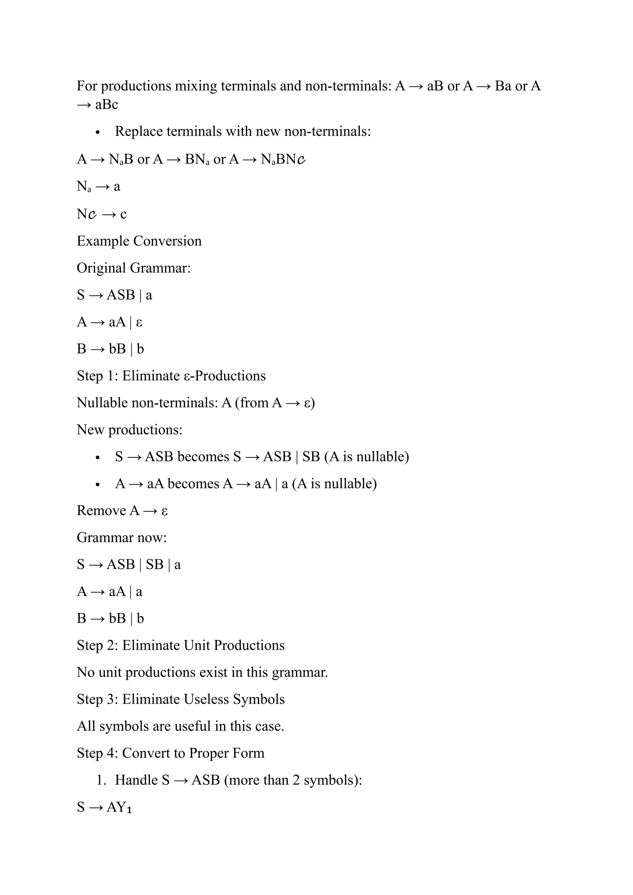
For productions mixing terminals and non-terminals: A → aB or A → Ba or A
→ aBc
 Replace terminals with new non-terminals:
A → N B or A → BN or A → N BN
ₐ ₐ ₐ 𝒸
N → a
ₐ
N𝒸 → c
Example Conversion
Original Grammar:
S → ASB | a
A → aA | ε
B → bB | b
Step 1: Eliminate ε-Productions
Nullable non-terminals: A (from A → ε)
New productions:
 S → ASB becomes S → ASB | SB (A is nullable)
 A → aA becomes A → aA | a (A is nullable)
Remove A → ε
Grammar now:
S → ASB | SB | a
A → aA | a
B → bB | b
Step 2: Eliminate Unit Productions
No unit productions exist in this grammar.
Step 3: Eliminate Useless Symbols
All symbols are useful in this case.
Step 4: Convert to Proper Form
1. Handle S → ASB (more than 2 symbols):
S → AY₁

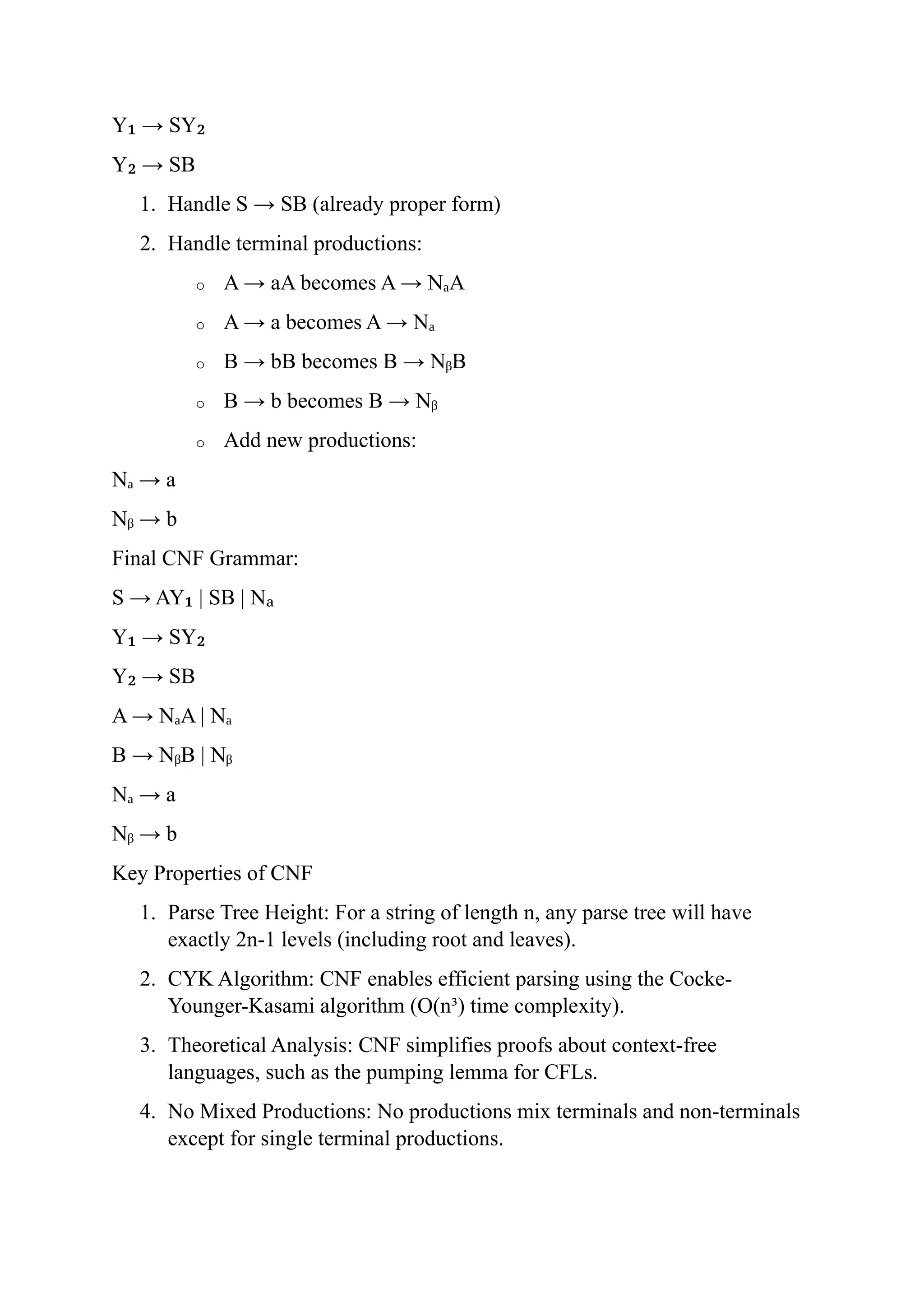
Y → SY
₁ ₂
Y → SB
₂
1. Handle S → SB (already proper form)
2. Handle terminal productions:
o A → aA becomes A → N A
ₐ
o A → a becomes A → Nₐ
o B → bB becomes B → N B
ᵦ
o B → b becomes B → Nᵦ
o Add new productions:
N → a
ₐ
N → b
ᵦ
Final CNF Grammar:
S → AY | SB | N
₁ ₐ
Y → SY
₁ ₂
Y → SB
₂
A → N A | N
ₐ ₐ
B → N B | N
ᵦ ᵦ
N → a
ₐ
N → b
ᵦ
Key Properties of CNF
1. Parse Tree Height: For a string of length n, any parse tree will have
exactly 2n-1 levels (including root and leaves).
2. CYK Algorithm: CNF enables efficient parsing using the Cocke-
Younger-Kasami algorithm (O(n³) time complexity).
3. Theoretical Analysis: CNF simplifies proofs about context-free
languages, such as the pumping lemma for CFLs.
4. No Mixed Productions: No productions mix terminals and non-terminals
except for single terminal productions.

*** Greibach Normal form: Greibach Normal Form is a stricter normal form
than Chomsky Normal Form where every production rule has a specific form
that makes it particularly useful for parsing and theoretical analysis.
Definition of Greibach Normal Form
A CFG is in Greibach Normal Form if every production rule is of the form:
A → aα
where:
 a is a single terminal symbol (∈ Σ)
 α is a (possibly empty) string of non-terminal symbols (∈ N*)
 No ε-productions are allowed (except possibly S → ε if ε is in the
language)
Key Properties of GNF
1. Leftmost Derivation: In GNF, every derivation step introduces exactly
one terminal symbol at the leftmost position
2. Deterministic Parsing: Enables efficient parsing with pushdown automata
3. Pumping Lemma: Used in proofs of the pumping lemma for context-free
languages
4. No Left Recursion: The grammar cannot have any direct or indirect left
recursion
Conversion Algorithm to GNF
Step 1: Convert to Chomsky Normal Form (CNF)
First bring the grammar to CNF (eliminate ε-productions, unit productions, etc.)
Step 2: Eliminate Left Recursion
For each non-terminal A with left-recursive productions:
1. Group productions as A → Aα | ... | Aα | β | ... | β (where β don't start
₁ ₘ ₁ ₙ ᵢ
with A)
2. Replace with:
A → β | ... | β | β Z | ... | β Z
₁ ₙ ₁ ₙ
Z → α | ... | α | α Z | ... | α Z
₁ ₘ ₁ ₘ
1. (where Z is a new non-terminal)

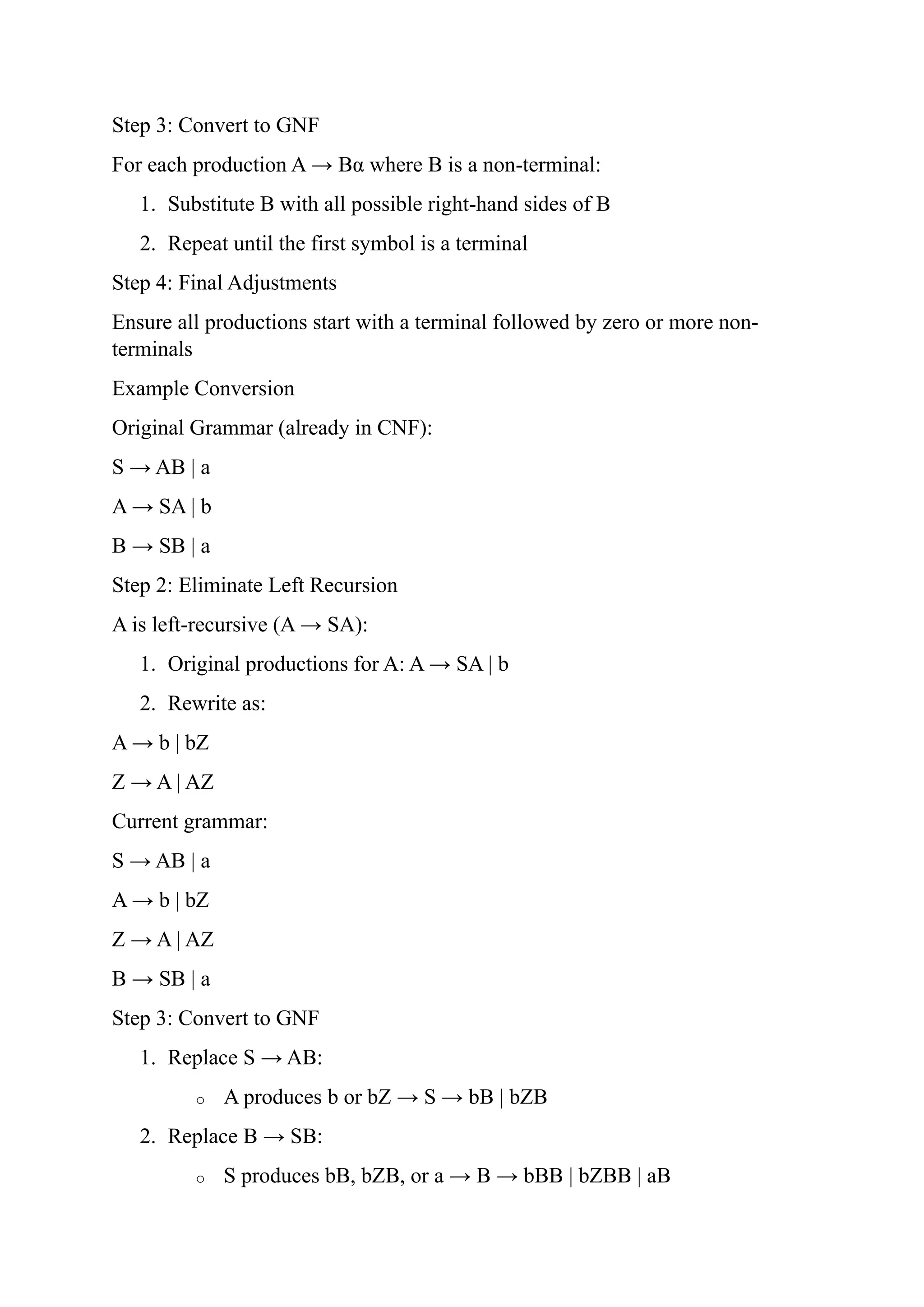
Step 3: Convert to GNF
For each production A → Bα where B is a non-terminal:
1. Substitute B with all possible right-hand sides of B
2. Repeat until the first symbol is a terminal
Step 4: Final Adjustments
Ensure all productions start with a terminal followed by zero or more non-
terminals
Example Conversion
Original Grammar (already in CNF):
S → AB | a
A → SA | b
B → SB | a
Step 2: Eliminate Left Recursion
A is left-recursive (A → SA):
1. Original productions for A: A → SA | b
2. Rewrite as:
A → b | bZ
Z → A | AZ
Current grammar:
S → AB | a
A → b | bZ
Z → A | AZ
B → SB | a
Step 3: Convert to GNF
1. Replace S → AB:
o A produces b or bZ → S → bB | bZB
2. Replace B → SB:
o S produces bB, bZB, or a → B → bBB | bZBB | aB

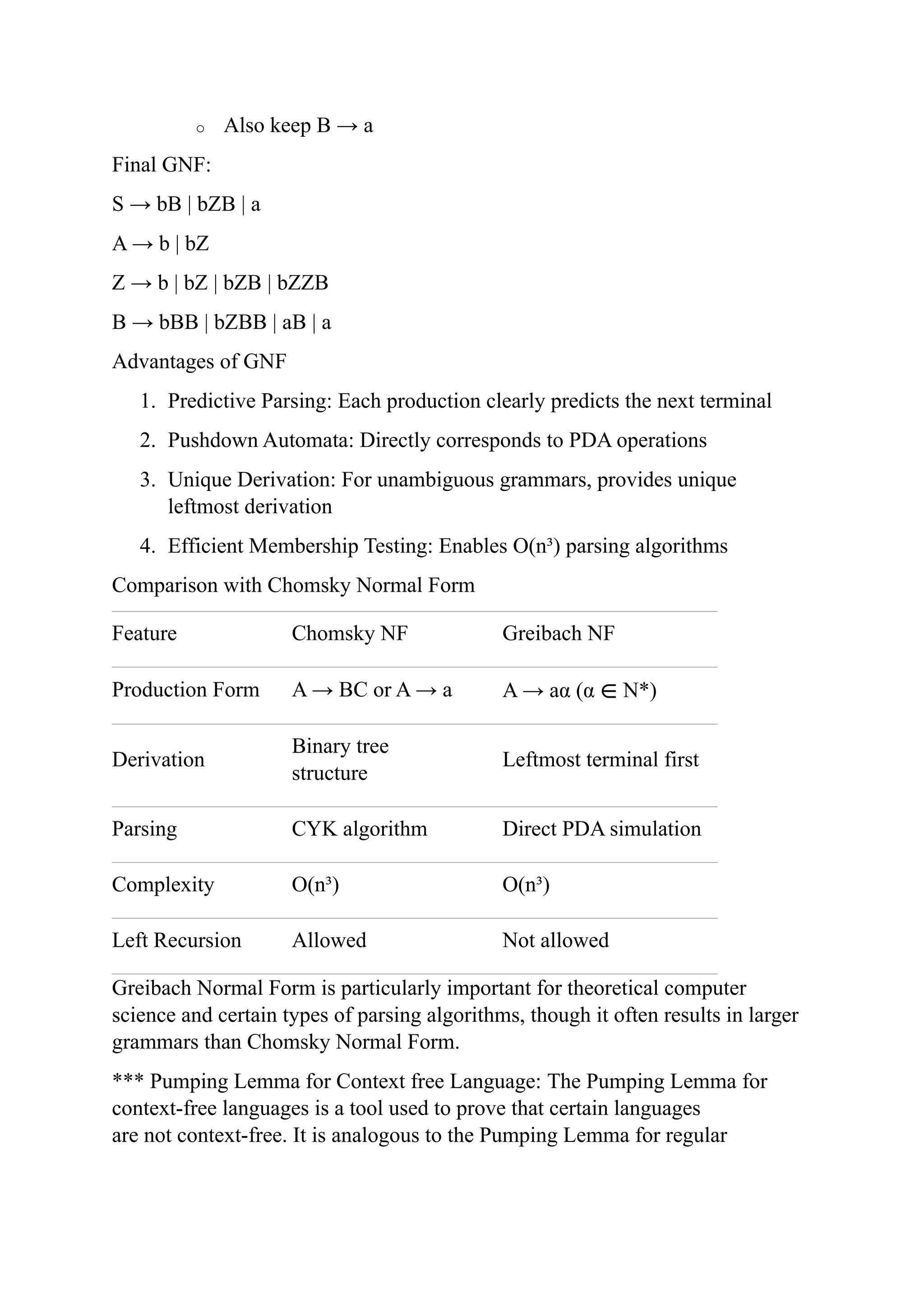
o Also keep B → a
Final GNF:
S → bB | bZB | a
A → b | bZ
Z → b | bZ | bZB | bZZB
B → bBB | bZBB | aB | a
Advantages of GNF
1. Predictive Parsing: Each production clearly predicts the next terminal
2. Pushdown Automata: Directly corresponds to PDA operations
3. Unique Derivation: For unambiguous grammars, provides unique
leftmost derivation
4. Efficient Membership Testing: Enables O(n³) parsing algorithms
Comparison with Chomsky Normal Form
Feature Chomsky NF Greibach NF
Production Form A → BC or A → a A → aα (α ∈ N*)
Derivation
Binary tree
structure
Leftmost terminal first
Parsing CYK algorithm Direct PDA simulation
Complexity O(n³) O(n³)
Left Recursion Allowed Not allowed
Greibach Normal Form is particularly important for theoretical computer
science and certain types of parsing algorithms, though it often results in larger
grammars than Chomsky Normal Form.
*** Pumping Lemma for Context free Language: The Pumping Lemma for
context-free languages is a tool used to prove that certain languages
are not context-free. It is analogous to the Pumping Lemma for regular

languages but is more complex due to the stack-based nature of pushdown
automata (PDAs).
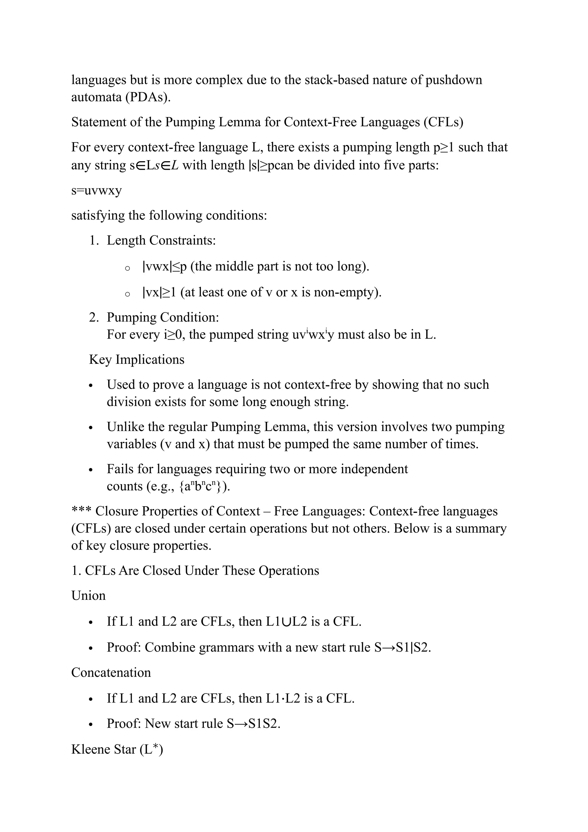
Statement of the Pumping Lemma for Context-Free Languages (CFLs)
For every context-free language L, there exists a pumping length p≥1 such that
any string s∈Ls∈L with length ∣s∣≥pcan be divided into five parts:
s=uvwxy
satisfying the following conditions:
1. Length Constraints:
o ∣vwx∣≤p (the middle part is not too long).
o ∣vx∣≥1 (at least one of v or x is non-empty).
2. Pumping Condition:
For every i≥0, the pumped string uvi
wxi
y must also be in L.
Key Implications
 Used to prove a language is not context-free by showing that no such
division exists for some long enough string.
 Unlike the regular Pumping Lemma, this version involves two pumping
variables (v and x) that must be pumped the same number of times.
 Fails for languages requiring two or more independent
counts (e.g., {an
bn
cn
}).
*** Closure Properties of Context – Free Languages: Context-free languages
(CFLs) are closed under certain operations but not others. Below is a summary
of key closure properties.
1. CFLs Are Closed Under These Operations
Union
 If L1 and L2 are CFLs, then L1∪L2 is a CFL.
 Proof: Combine grammars with a new start rule S→S1∣S2.
Concatenation
 If L1 and L2 are CFLs, then L1⋅L2 is a CFL.
 Proof: New start rule S→S1S2.
Kleene Star (L∗
)

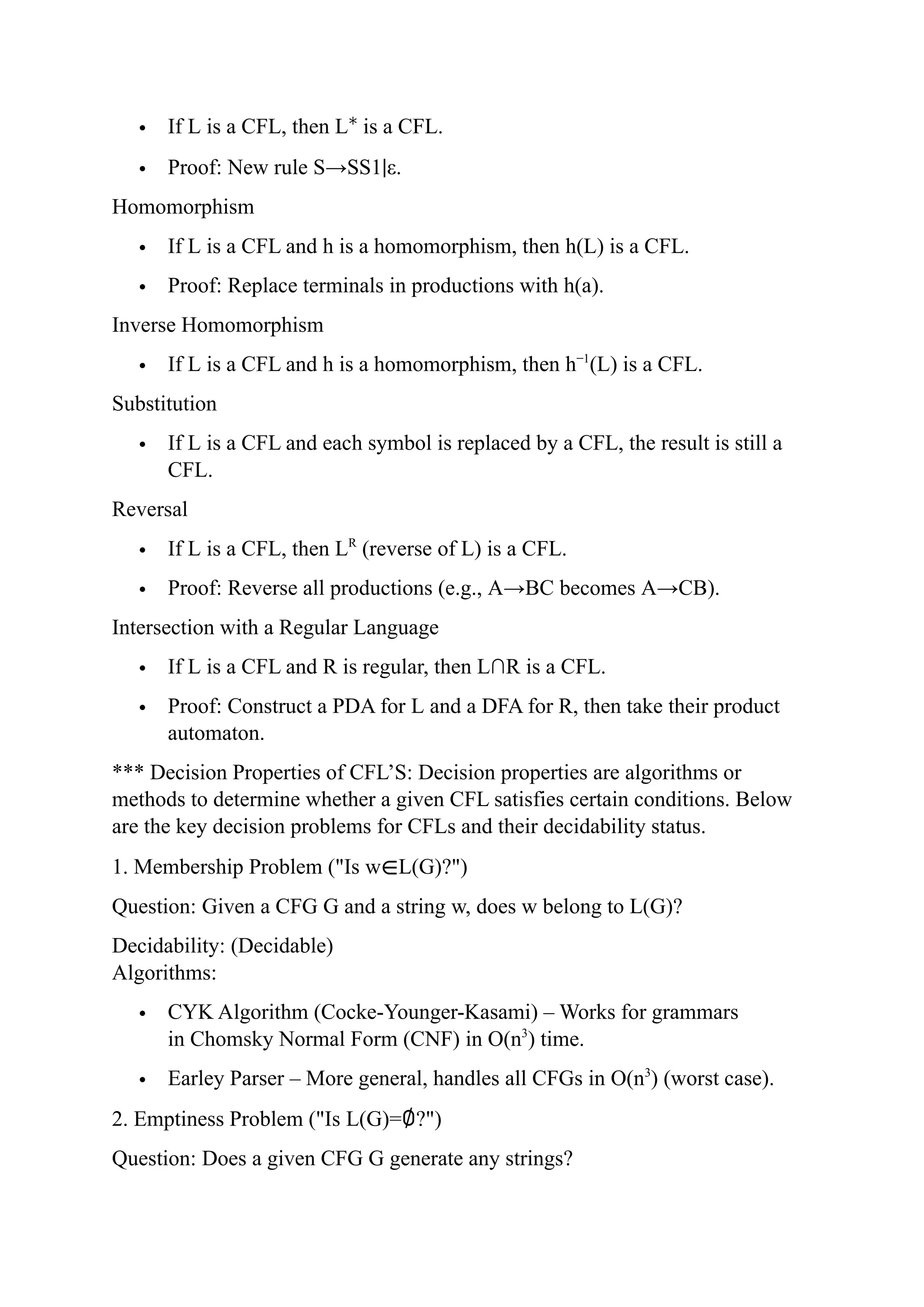
 If L is a CFL, then L∗
is a CFL.
 Proof: New rule S→SS1∣ε.
Homomorphism
 If L is a CFL and h is a homomorphism, then h(L) is a CFL.
 Proof: Replace terminals in productions with h(a).
Inverse Homomorphism
 If L is a CFL and h is a homomorphism, then h−1
(L) is a CFL.
Substitution
 If L is a CFL and each symbol is replaced by a CFL, the result is still a
CFL.
Reversal
 If L is a CFL, then LR
(reverse of L) is a CFL.
 Proof: Reverse all productions (e.g., A→BC becomes A→CB).
Intersection with a Regular Language
 If L is a CFL and R is regular, then L∩R is a CFL.
 Proof: Construct a PDA for L and a DFA for R, then take their product
automaton.
*** Decision Properties of CFL’S: Decision properties are algorithms or
methods to determine whether a given CFL satisfies certain conditions. Below
are the key decision problems for CFLs and their decidability status.
1. Membership Problem ("Is w∈L(G)?")
Question: Given a CFG G and a string w, does w belong to L(G)?
Decidability: (Decidable)
Algorithms:
 CYK Algorithm (Cocke-Younger-Kasami) – Works for grammars
in Chomsky Normal Form (CNF) in O(n3
) time.
 Earley Parser – More general, handles all CFGs in O(n3
) (worst case).
2. Emptiness Problem ("Is L(G)=∅?")
Question: Does a given CFG G generate any strings?

Decidability: (Decidable)
Algorithm:
 Perform a reachability analysis on the production rules:
o Mark all terminals as "generating."
o If a non-terminal A has a rule A→α where all symbols in α are
generating, mark A as generating.
o Repeat until no new non-terminals are marked.
o If the start symbol S is generating, L(G)≠∅; otherwise, it is empty.
3. Finiteness Problem ("Is L(G) finite?")
Question: Does a given CFG G generate a finite number of strings?
Decidability: Yes (Decidable)
Algorithm:
1. Convert the grammar to Chomsky Normal Form (CNF).
2. Construct the dependency graph where nodes are non-terminals and
edges represent productions (e.g., A→BC implies
edges A→B and A→C).
3. Check for cycles in the graph:
o If a cycle exists, the language is infinite (due to recursive
derivations).
o If no cycles exist, the language is finite.
***introduction to Turing Machines: A Turing Machine (TM) is a theoretical
computing device introduced by Alan Turing (1936) to formalize the concept of
computation. It is the most powerful model in automata theory and serves as the
foundation of modern computer science.
What is a Turing Machine?
A Turing Machine is a mathematical model consisting of:
 An infinite tape divided into cells (each holding a symbol).
 A tape head that reads/writes symbols and moves left/right.
 A finite set of states (including an initial and accepting/rejecting states).
 A transition function that determines the machine's behavior.

Unlike finite automata or pushdown automata, a TM has unlimited
memory (due to the infinite tape) and can simulate any algorithm.
2. Formal Definition
A Turing Machine is a 7-tuple:
M=(Q,Σ,Γ,δ,q0,qaccept,qreject)
where:
 Q = Finite set of states
 Σ = Input alphabet (excluding the blank symbol ␣)
 Γ = Tape alphabet (includes Σ∪{␣})
 Δ = Transition function: Q×Γ→Q×Γ×{L,R}
 q0 = Start state
 qaccept = Accepting state
 qreject = Rejecting state
3. How a Turing Machine Works
1. Initialization:
o The input string is written on the tape, surrounded by blanks (␣).
o The head starts at the leftmost symbol.
o The machine begins in state q0.
2. Computation Steps:
o Reads the symbol under the head.
o Consults δ to determine:
 New state,
 Symbol to write,
 Whether to move Left (L) or Right (R).
o Repeats until it reaches qaccept or qreject.
3. Halting:
o If qaccept is reached → Input accepted.

o If qreject is reached → Input rejected.
o If it runs forever → Loop (no decision).
Construct a Turing Machine for L = a^n b^n n ≥ 1
Formal Definition of Turing Machine
A Turing machine can be formally described as seven tuples
(Q,X, Σ, δ,q0,B,F)
Where,
 Q is a finite set of states
 X is the tape alphabet
 Σ is the input alphabet
 δ is a transition function: δ:QxX→QxXx{left shift, right shift}
 q0 is the initial state
 B is the blank symbol
 F is the final state.
A Turing Machine (TM) is a mathematical model which consists of an infinite
length tape divided into cells on which input is given. It consists of a head
which reads the input tape. A state register stores the state of the Turing
machine.
After reading an input symbol, it is replaced with another symbol, its internal
state is changed, and it moves from one cell to the right or left. If the TM
reaches the final state, the input string is accepted, otherwise rejected.
The Turing machine has a read/write head. So we can write on the tape.
Now, let us construct a Turing machine which accepts equal number of a’s and
b’s,
The language it is generated is L ={ an
bn
| n>=1}, the strings that are accepted
by the given language is −
L= {ab, aabb, aaabbb, aaaabbbb,………}
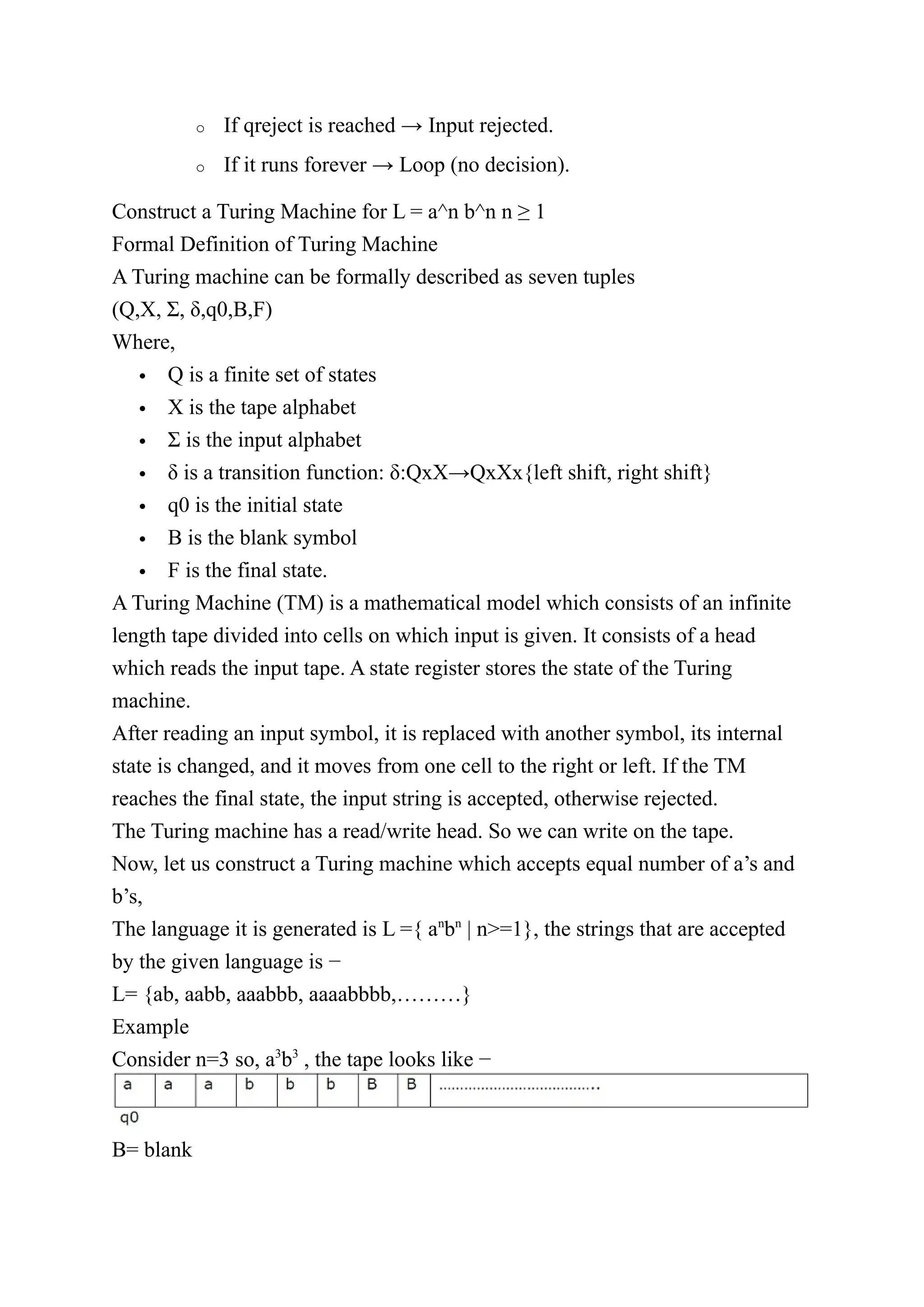
Example
Consider n=3 so, a3
b3
, the tape looks like −
B= blank

We need to convert every ‘a’ as X and every ‘b’ as Y. If the Turing machine
contains an equal number of X and Y then it reaches the final state.
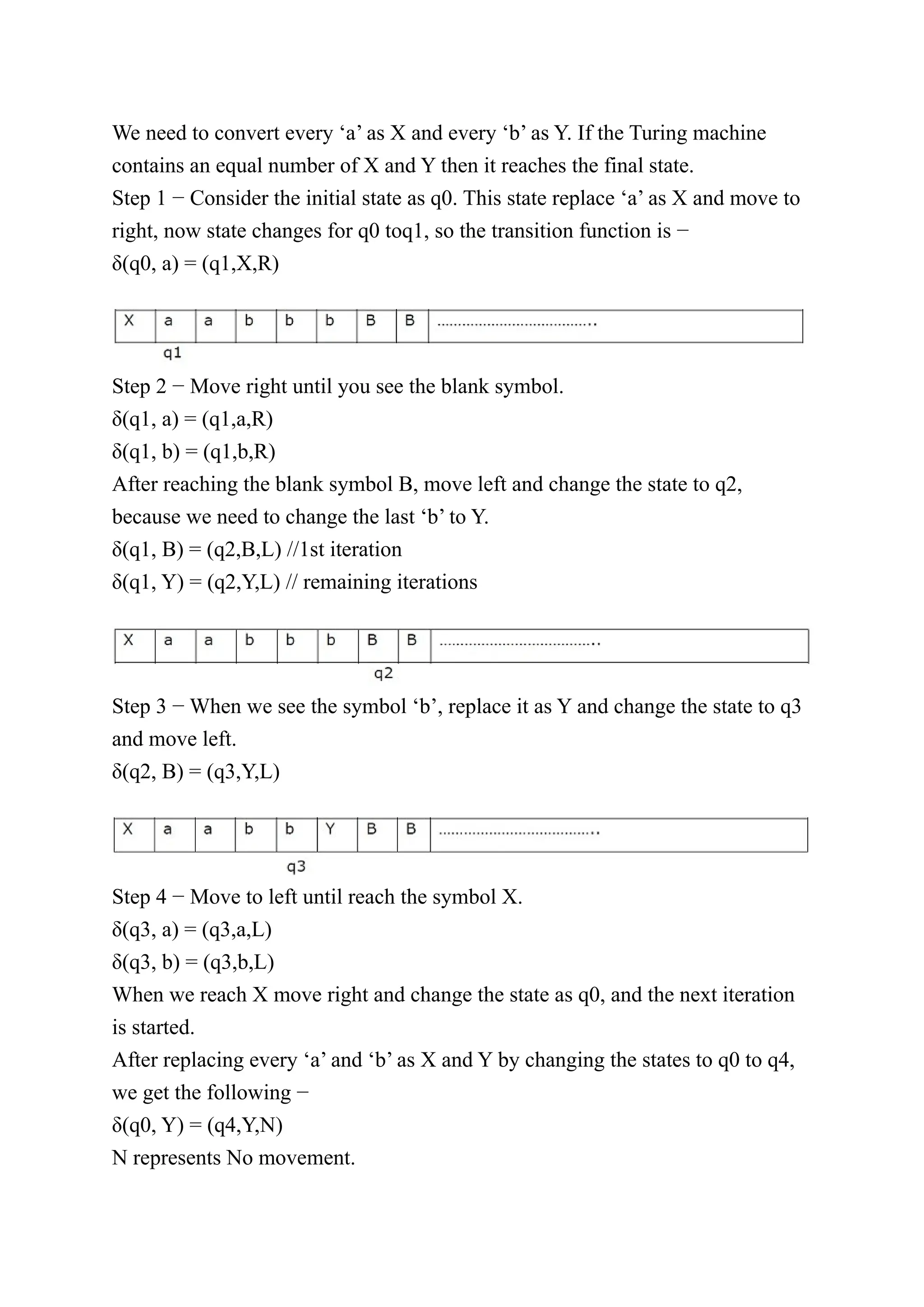
Step 1 − Consider the initial state as q0. This state replace ‘a’ as X and move to
right, now state changes for q0 toq1, so the transition function is −
δ(q0, a) = (q1,X,R)
Step 2 − Move right until you see the blank symbol.
δ(q1, a) = (q1,a,R)
δ(q1, b) = (q1,b,R)
After reaching the blank symbol B, move left and change the state to q2,
because we need to change the last ‘b’ to Y.
δ(q1, B) = (q2,B,L) //1st iteration
δ(q1, Y) = (q2,Y,L) // remaining iterations
Step 3 − When we see the symbol ‘b’, replace it as Y and change the state to q3
and move left.
δ(q2, B) = (q3,Y,L)
Step 4 − Move to left until reach the symbol X.
δ(q3, a) = (q3,a,L)
δ(q3, b) = (q3,b,L)
When we reach X move right and change the state as q0, and the next iteration
is started.
After replacing every ‘a’ and ‘b’ as X and Y by changing the states to q0 to q4,
we get the following −
δ(q0, Y) = (q4,Y,N)
N represents No movement.

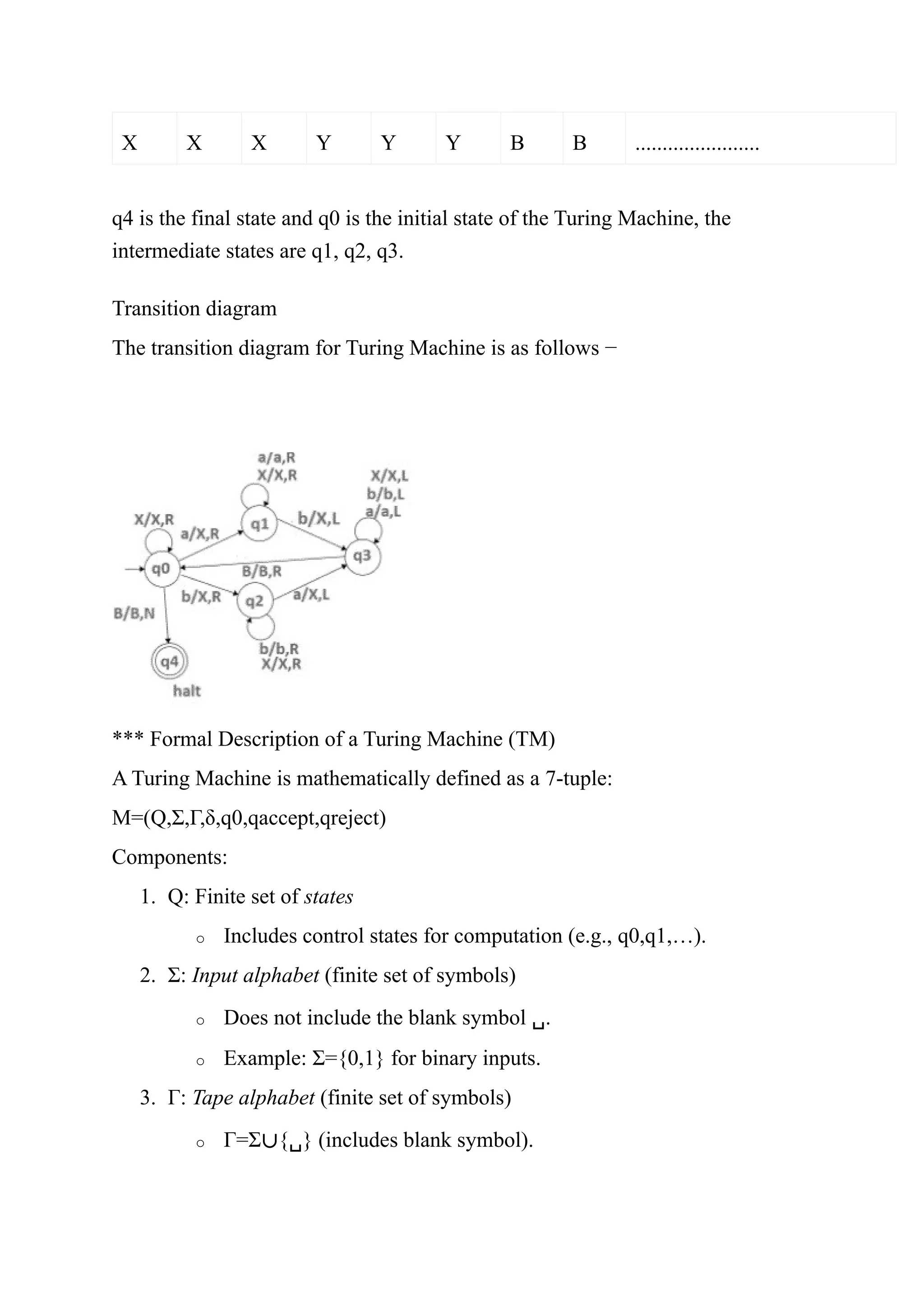
X X X Y Y Y B B .......................
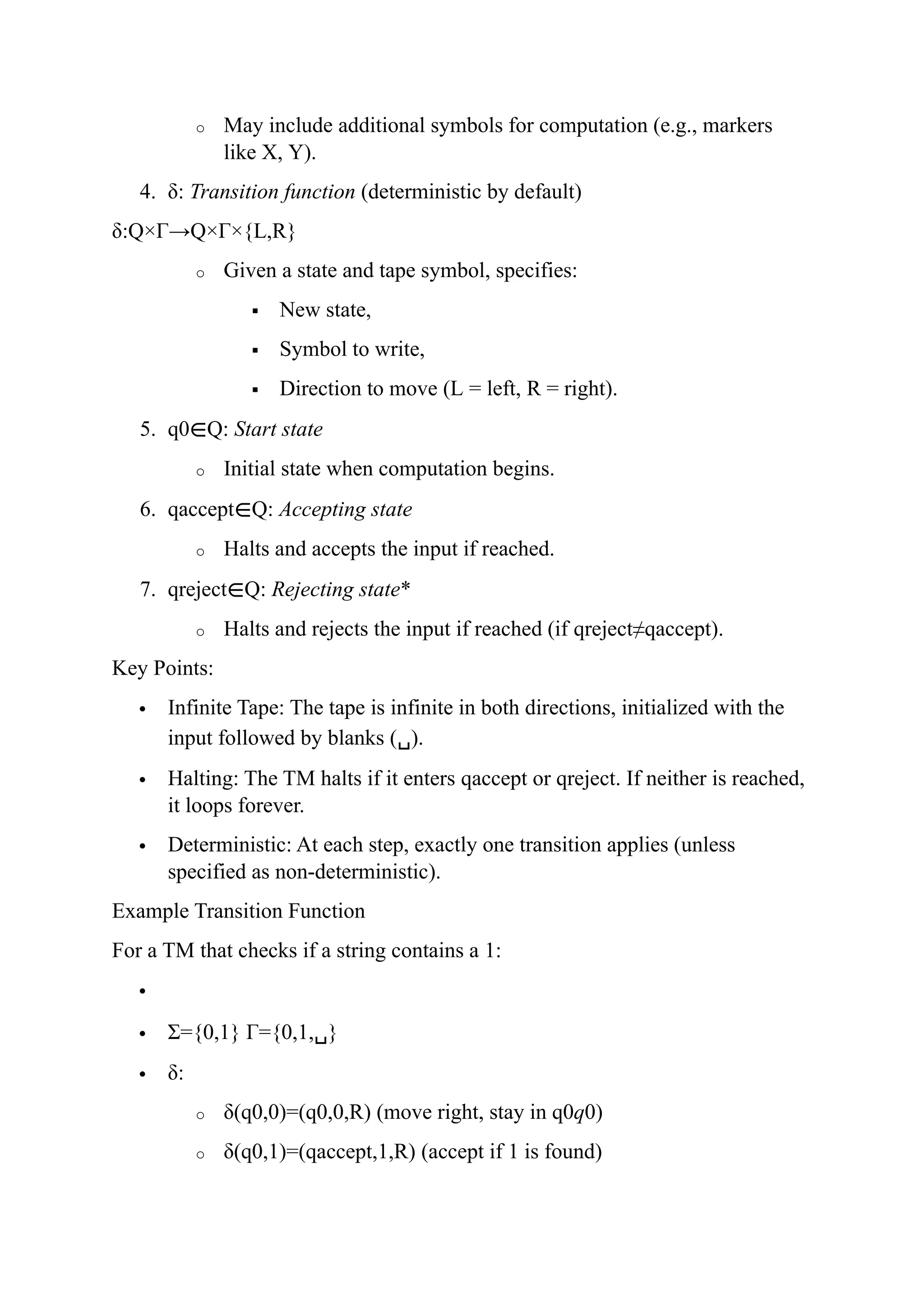
q4 is the final state and q0 is the initial state of the Turing Machine, the
intermediate states are q1, q2, q3.
Transition diagram
The transition diagram for Turing Machine is as follows −
*** Formal Description of a Turing Machine (TM)
A Turing Machine is mathematically defined as a 7-tuple:
M=(Q,Σ,Γ,δ,q0,qaccept,qreject)
Components:
1. Q: Finite set of states
o Includes control states for computation (e.g., q0,q1,…).
2. Σ: Input alphabet (finite set of symbols)
o Does not include the blank symbol ␣.
o Example: Σ={0,1} for binary inputs.
3. Γ: Tape alphabet (finite set of symbols)
o Γ=Σ∪{␣} (includes blank symbol).

o May include additional symbols for computation (e.g., markers
like X, Y).
4. δ: Transition function (deterministic by default)
δ:Q×Γ→Q×Γ×{L,R}
o Given a state and tape symbol, specifies:
 New state,
 Symbol to write,
 Direction to move (L = left, R = right).
5. q0∈Q: Start state
o Initial state when computation begins.
6. qaccept∈Q: Accepting state
o Halts and accepts the input if reached.
7. qreject∈Q: Rejecting state*
o Halts and rejects the input if reached (if qreject≠qaccept).
Key Points:
 Infinite Tape: The tape is infinite in both directions, initialized with the
input followed by blanks (␣).
 Halting: The TM halts if it enters qaccept or qreject. If neither is reached,
it loops forever.
 Deterministic: At each step, exactly one transition applies (unless
specified as non-deterministic).
Example Transition Function
For a TM that checks if a string contains a 1:

 Σ={0,1} Γ={0,1,␣}
 δ:
o δ(q0,0)=(q0,0,R) (move right, stay in q0q0)
o δ(q0,1)=(qaccept,1,R) (accept if 1 is found)

o δ(q0,␣)=(qreject,␣,R) (reject if no 1 is found)
*** Instantaneous description: An Instantaneous Description (ID) is a snapshot
of a Turing Machine's configuration at a given moment during computation. It
captures:
1. The current state of the TM.
2. The contents of the tape.
3. The position of the tape head.
Formal Definition
An ID is a triple:
αqβ
where:
 α∈Γ∗
: Tape symbols to the left of the head (excluding the current cell).
 q∈Q: Current state.
 β∈Γ∗
: Tape symbols from the current cell to the right (including the
current cell).
Conventions:
1. The tape head reads the leftmost symbol of β.
2. If β=ε (empty), the head is on a blank (␣).
Example IDs
For a TM with input 101 (tape: ␣101␣␣...) and head initially on 1:
 Initial ID: q0 101
(Head on 1, state q0, left of head is blank but omitted).
 After moving right: 1 q0 01
(Head on 0, state q0, left portion is 1).
Transition Between IDs
Let δ(q,a)=(p,b,L). For an ID:
α c q a β(head on ‘a‘, state q)
The next ID is:

α p c b β(writes ‘b‘, moves left to ‘c‘, transitions to state p)
Special Cases:
1. Leftmost cell move:
If head is at the left end (α=ε) and moves left, the ID becomes p ␣ b β.
2. Right move:
If δ(q,a)=(p,b,R), the next ID is α b p βαbpβ.
Example: TM for {0n1n∣n≥0}{0n1n∣n≥0}
Initial Tape: ␣0011␣␣...
Initial ID: q0 0011
Transition Steps:
1. δ(q0,0)=(q1,X,R)
Next ID: X q1 011
2. δ(q1,0)=(q1,0,R)
Next ID: X0 q1 11
3. δ(q1,1)=(q2,Y,L)
Next ID: X q2 0Y1
4. δ(q2,0)=(q2,0,L)
Next ID: q2 X0Y1
5. δ(q2,X)=(q0,X,R)
Next ID: X q0 0Y1
(Process repeats until all 0s and 1s are matched).
Key Properties
1. Deterministic Transitions: Each ID has at most one successor.
2. Accepting ID: Any ID containing qaccept.
3. Rejecting ID: Any ID containing qreject.
4. Halting: No transitions apply in qaccept or qreject.
*** The Language of a Turing Machine: A Turing Machine
(TM) recognizes or decides a language, defining its computational power. The

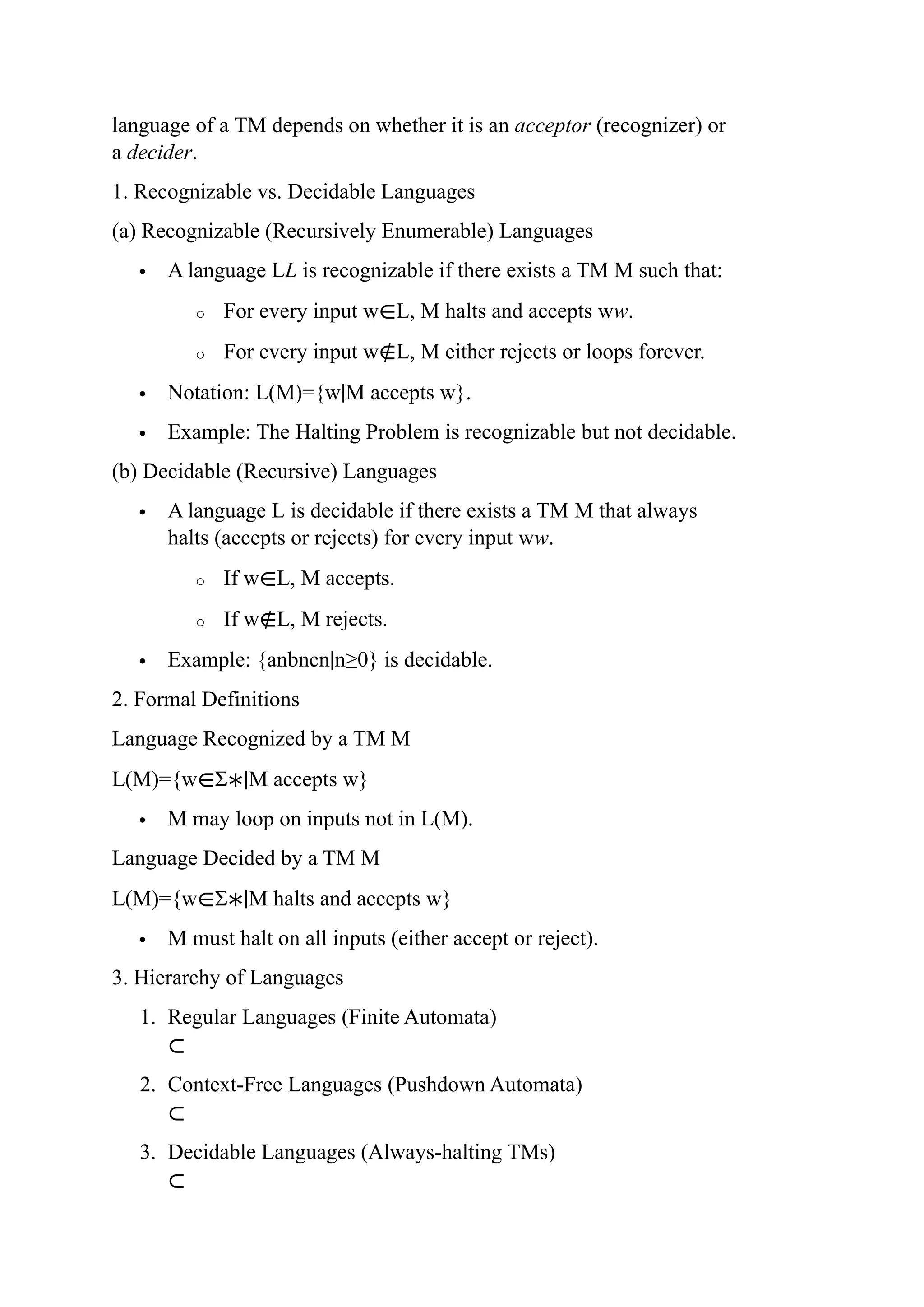
language of a TM depends on whether it is an acceptor (recognizer) or
a decider.
1. Recognizable vs. Decidable Languages
(a) Recognizable (Recursively Enumerable) Languages
 A language LL is recognizable if there exists a TM M such that:
o For every input w∈L, M halts and accepts ww.
o For every input w∉L, M either rejects or loops forever.
 Notation: L(M)={w∣M accepts w}.
 Example: The Halting Problem is recognizable but not decidable.
(b) Decidable (Recursive) Languages
 A language L is decidable if there exists a TM M that always
halts (accepts or rejects) for every input ww.
o If w∈L, M accepts.
o If w∉L, M rejects.
 Example: {anbncn∣n≥0} is decidable.
2. Formal Definitions
Language Recognized by a TM M
L(M)={w∈Σ∗∣M accepts w}
 M may loop on inputs not in L(M).
Language Decided by a TM M
L(M)={w∈Σ∗∣M halts and accepts w}
 M must halt on all inputs (either accept or reject).
3. Hierarchy of Languages
1. Regular Languages (Finite Automata)
⊂
2. Context-Free Languages (Pushdown Automata)
⊂
3. Decidable Languages (Always-halting TMs)
⊂

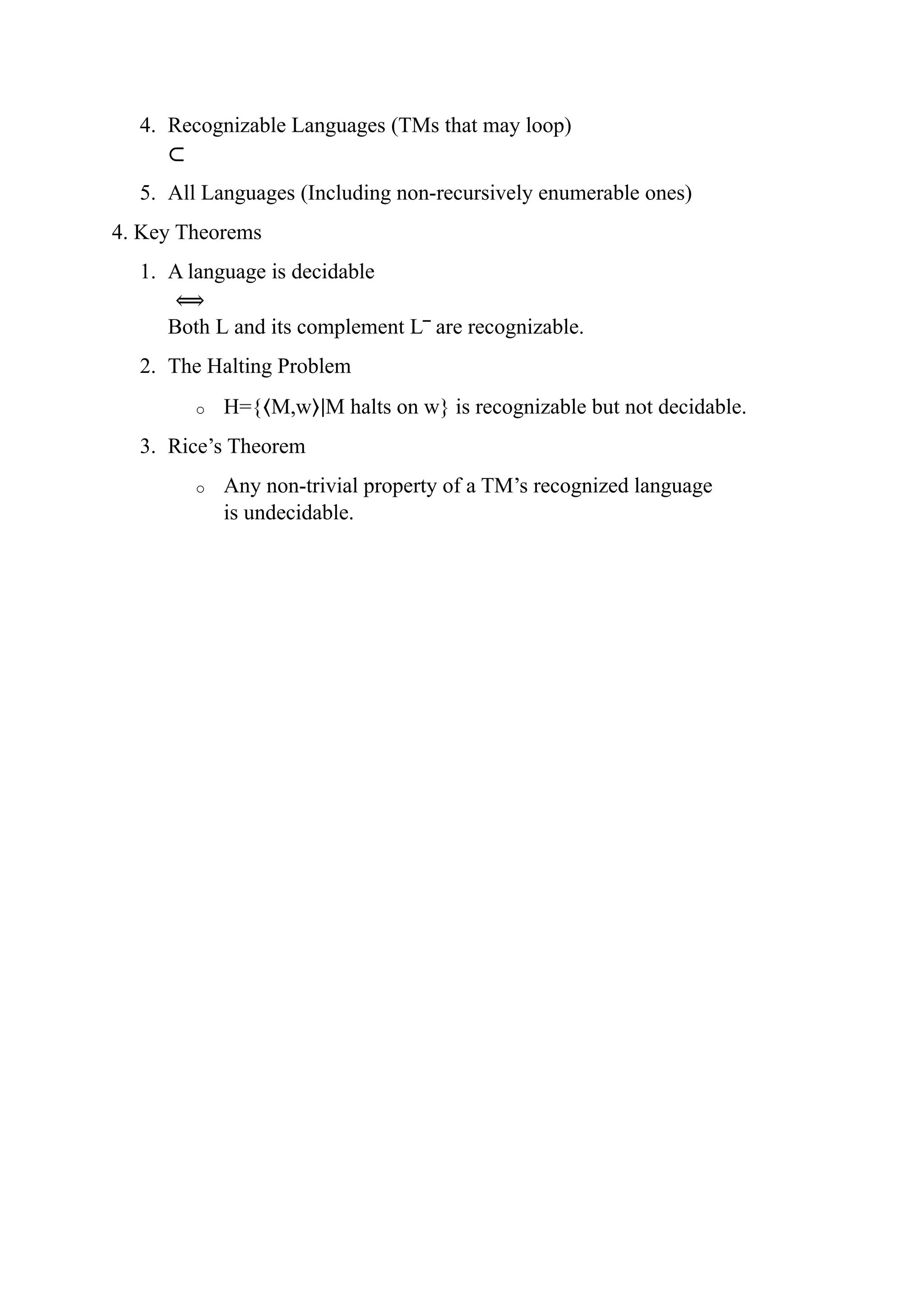
4. Recognizable Languages (TMs that may loop)
⊂
5. All Languages (Including non-recursively enumerable ones)
4. Key Theorems
1. A language is decidable
⟺
Both L and its complement L‾ are recognizable.
2. The Halting Problem
o H={⟨M,w⟩∣M halts on w} is recognizable but not decidable.
3. Rice’s Theorem
o Any non-trivial property of a TM’s recognized language
is undecidable.

Normal Forms for Context Free Grammers.docx

More Related Content

Similar to Normal Forms for Context Free Grammers.docx

More from SUNEEL37

Recently uploaded

Normal Forms for Context Free Grammers.docx