Neural Network

1. UNIT 2
DEEP LEARNING

12. Perceptron
• A perceptron is a simple binary classification algorithm, proposed by Cornell scientist Frank Rosenblatt.
• It helps to divide a set of input signals into two parts—“yes” and “no”.
• But unlike many other classification algorithms, the perceptron was modeled after the essential unit of
the human brain—the neuron and has an uncanny ability to learn and solve complex problems.
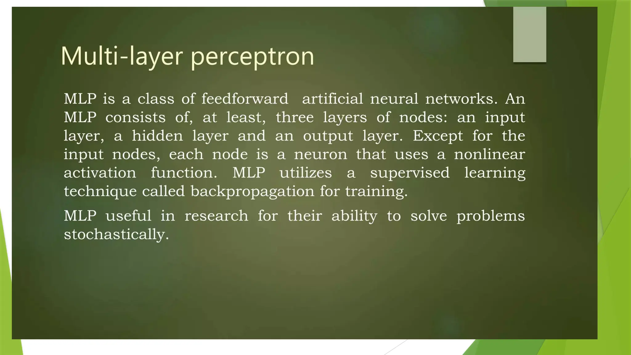
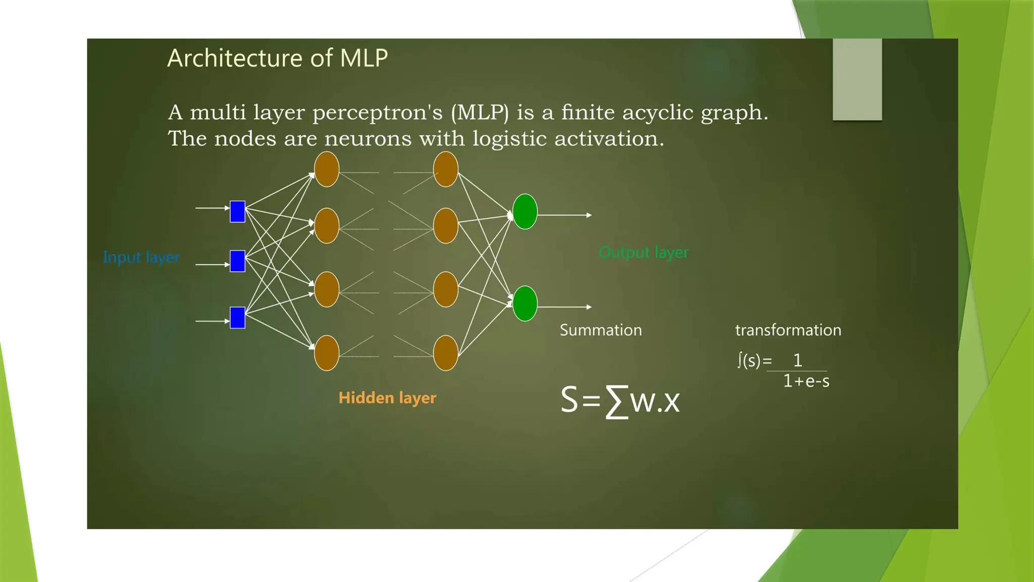
Multi-layer Perceptron
Multi-layer perception is also known as MLP.
It is fully connected dense layers, which transform any input dimension to the desired dimension.
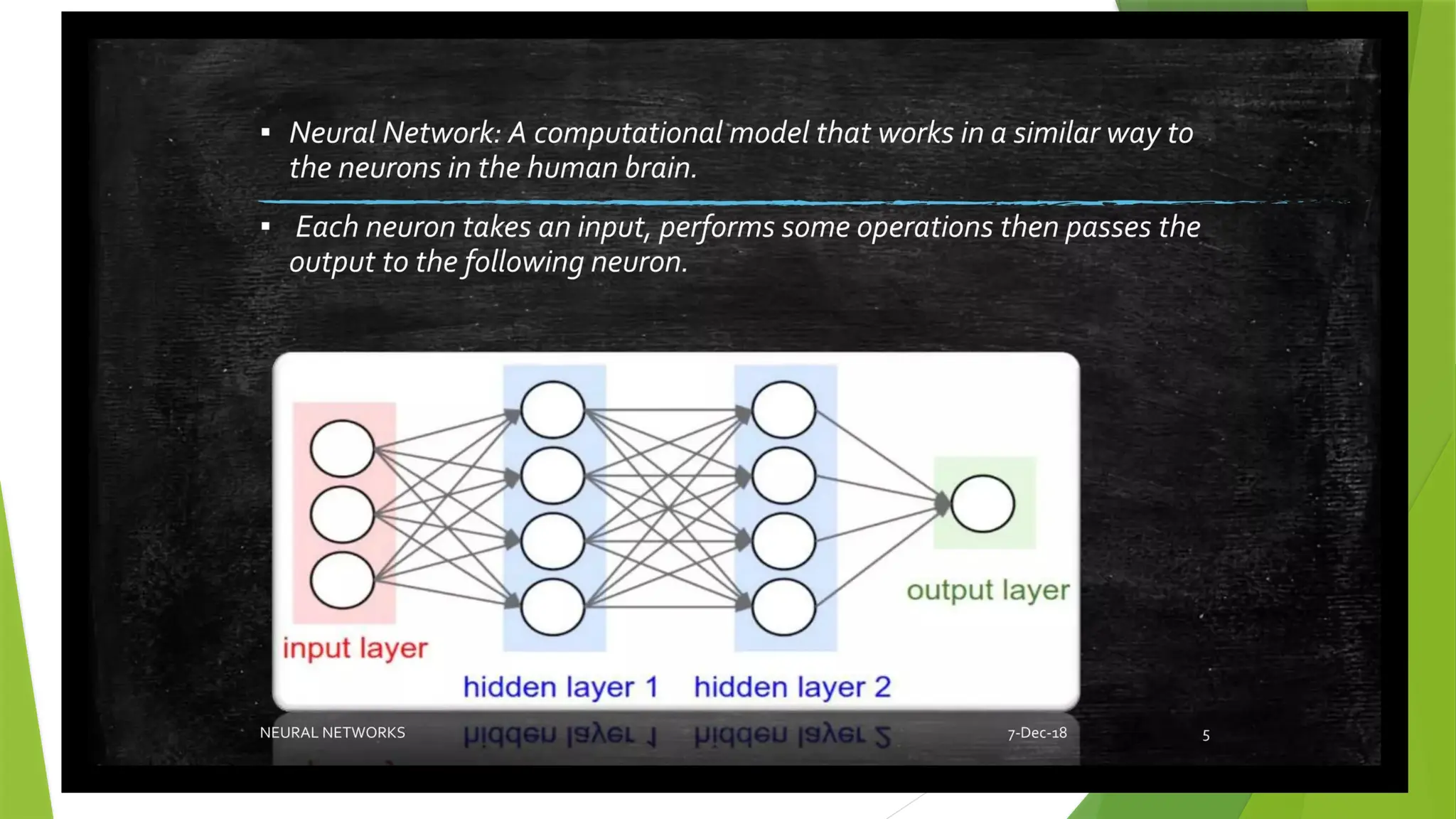
A multi-layer perception is a neural network that has multiple layers.
To create a neural network we combine neurons together so that the outputs of some neurons are
inputs of other neurons.

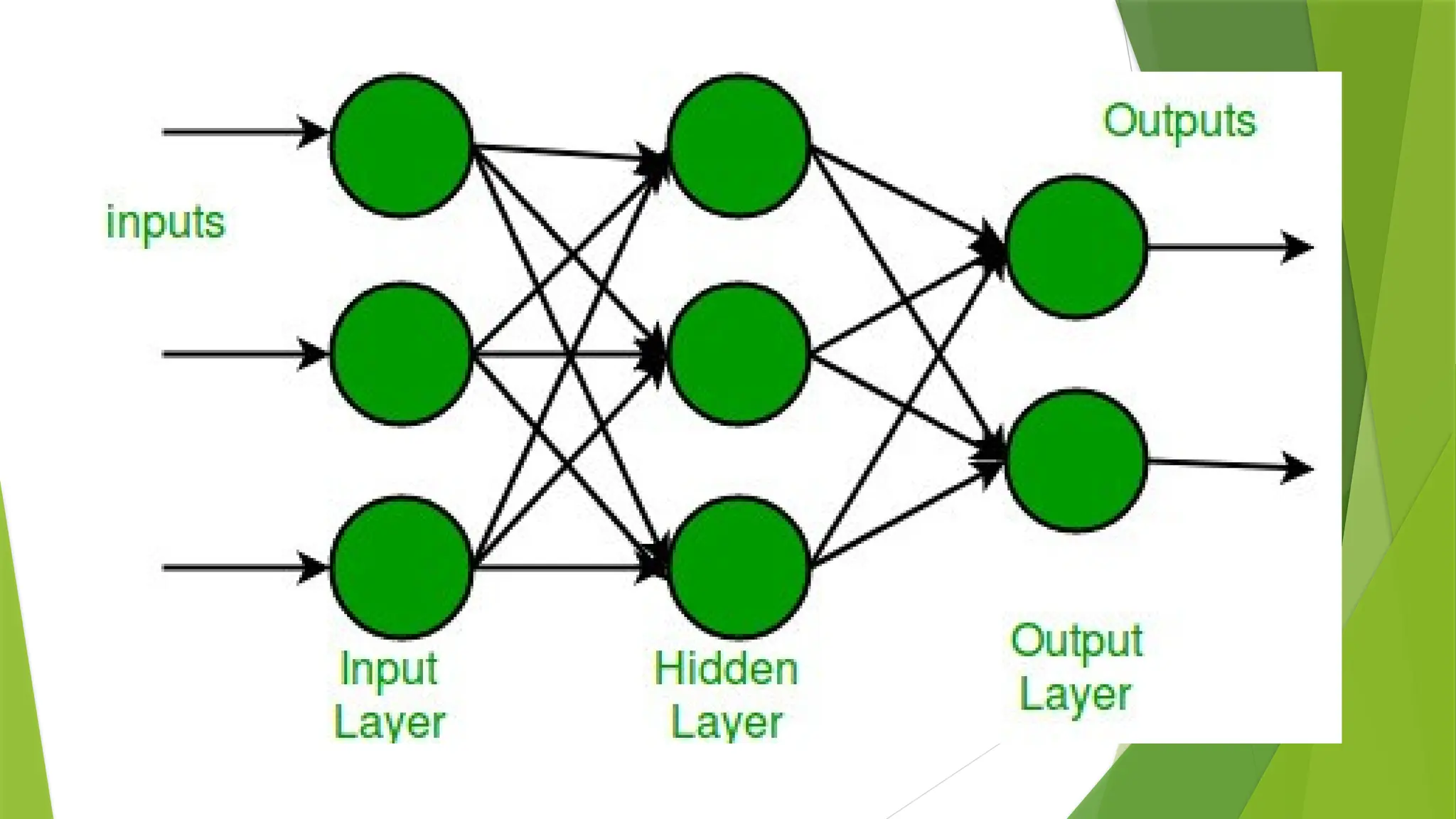
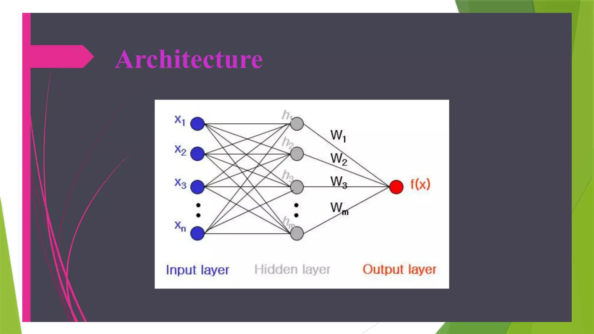
14. In the multi-layer perceptron diagram above, we can see that there are three inputs and thus three input
nodes and the hidden layer has three nodes.
The output layer gives two outputs, therefore there are two output nodes.
The nodes in the input layer take input and forward it for further process, in the diagram above the nodes
in the input layer forwards their output to each of the three nodes in the hidden layer,
and in the same way, the hidden layer processes the information and passes it to the output layer.
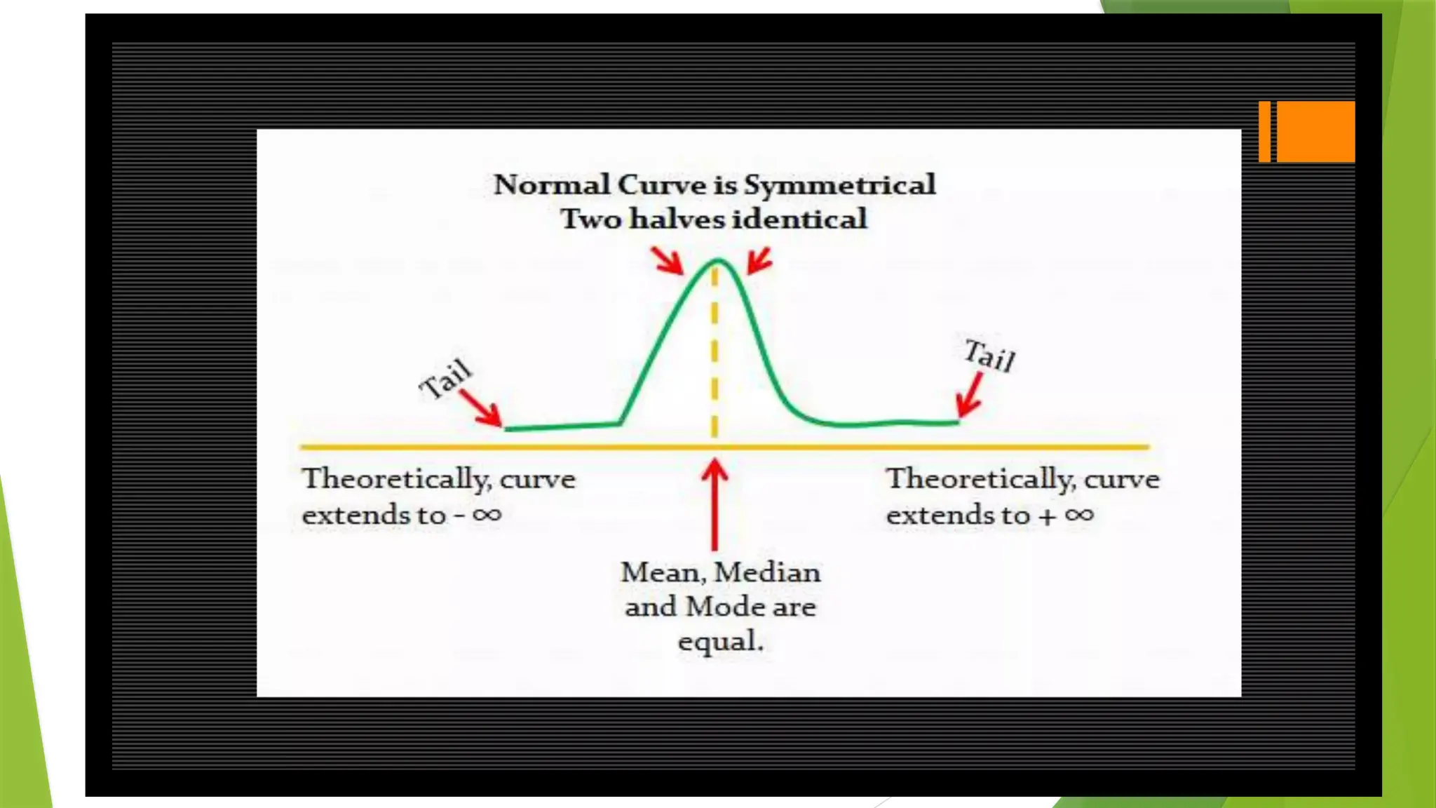
Every node in the multi-layer perception uses a sigmoid activation function.
The sigmoid activation function takes real values as input and converts them to numbers between 0 and 1
using the sigmoid formula.
α(x) = 1/( 1 + exp(-x))

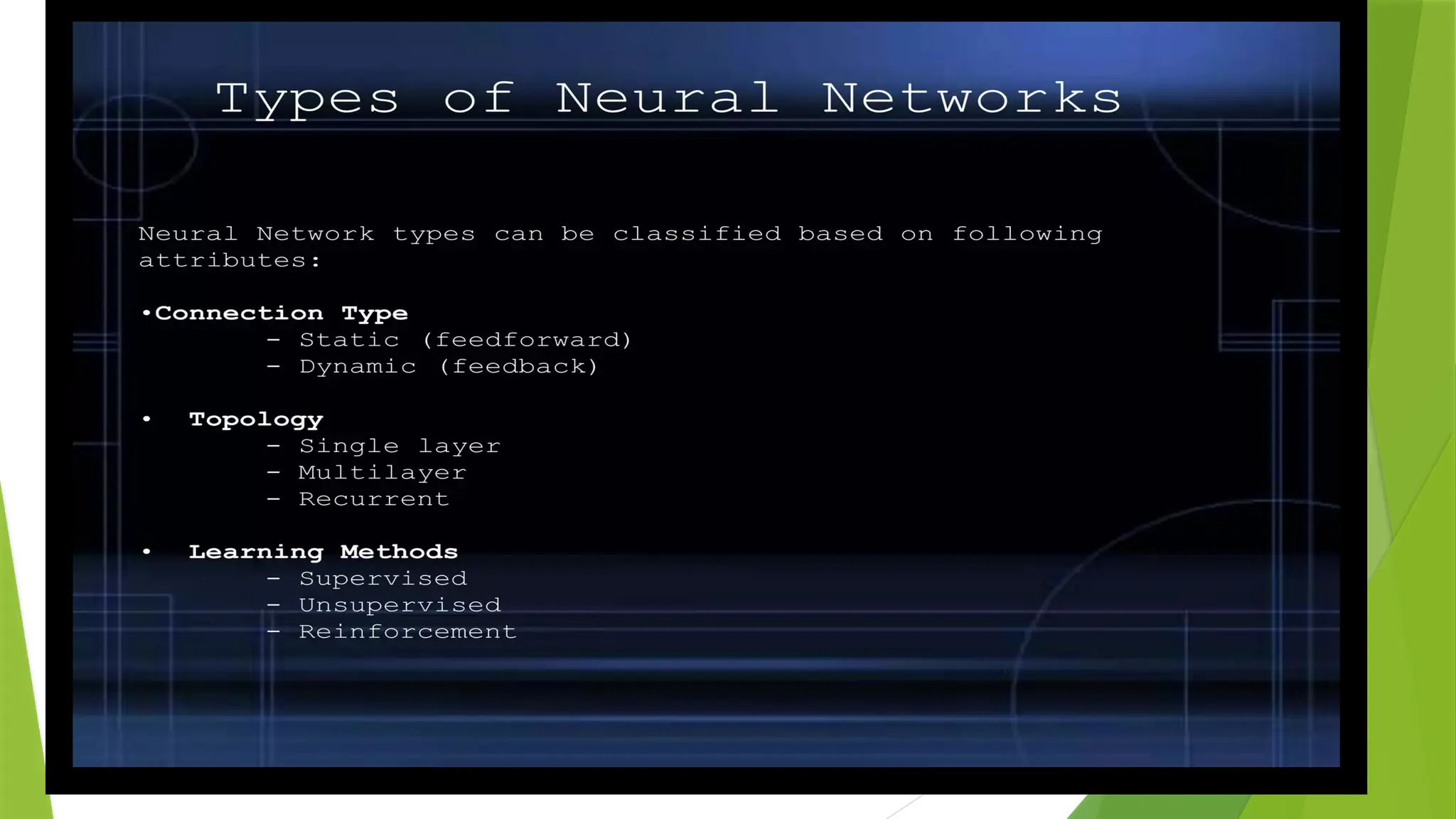
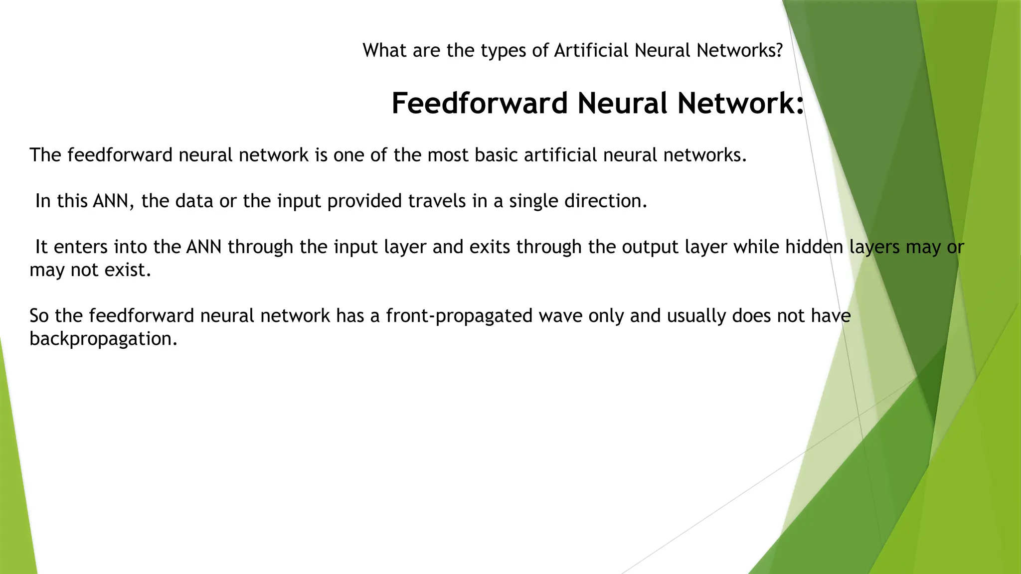
15. What are the types of Artificial Neural Networks?
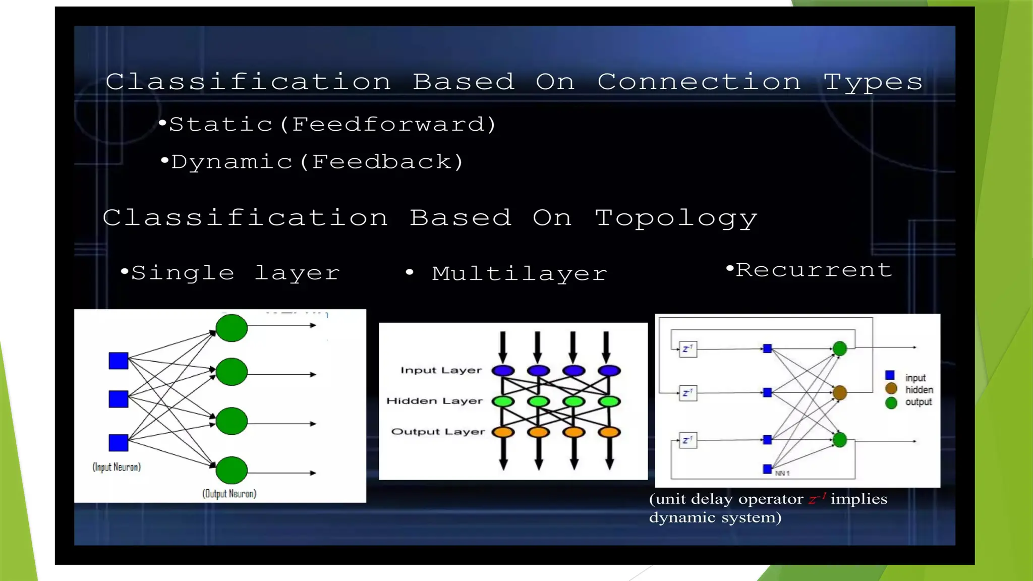
Feedforward Neural Network:
The feedforward neural network is one of the most basic artificial neural networks.
In this ANN, the data or the input provided travels in a single direction.
It enters into the ANN through the input layer and exits through the output layer while hidden layers may or
may not exist.
So the feedforward neural network has a front-propagated wave only and usually does not have
backpropagation.

16. MULTILAYER FEEDFORWARD NEURAL NETWORK

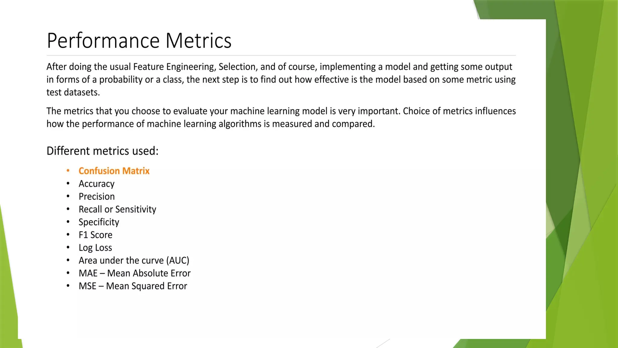
26. Performance metrics are a part of every machine learning pipeline.
They tell you if you’re making progress, and put a number on it. All machine learning models, whether it’s linear
regression, or a SOTA technique like BERT, need a metric to judge performance.
Every machine learning task can be broken down to either Regression or Classification, just like the performance
metrics. There are dozens of metrics for both problems, but we’re gonna discuss popular ones along with what
information they provide about model performance. It’s important to know how your model sees your data!
If you ever participated in a Kaggle competition, you probably noticed the evaluation section. More often than
not, there’s a metric on which they judge your performance.
Metrics are different from loss functions. Loss functions show a measure of model performance. They’re used to
train a machine learning model (using some kind of optimization like Gradient Descent), and they’re usually
differentiable in the model’s parameters.
Metrics are used to monitor and measure the performance of a model (during training and testing), and
don’t need to be differentiable.

27. What is hyper parameter optimization?
Before I define hyper parameter optimization, you need to understand what a hyper parameter is.
In short, hyper parameters are different parameter values that are used to control the learning process and
have a significant effect on the performance of machine learning models.
An example of hyper parameters in the Random Forest algorithm is the number of estimators (n_estimators),
maximum depth (max_depth), and criterion. These parameters are tunable and can directly affect how well a
model trains.
So then hyper parameter optimization is the process of finding the right combination of hyper parameter
values to achieve maximum performance on the data in a reasonable amount of time.
This process plays a vital role in the prediction accuracy of a machine learning algorithm. Therefore Hyper
parameter optimization is considered the trickiest part of building machine learning models.

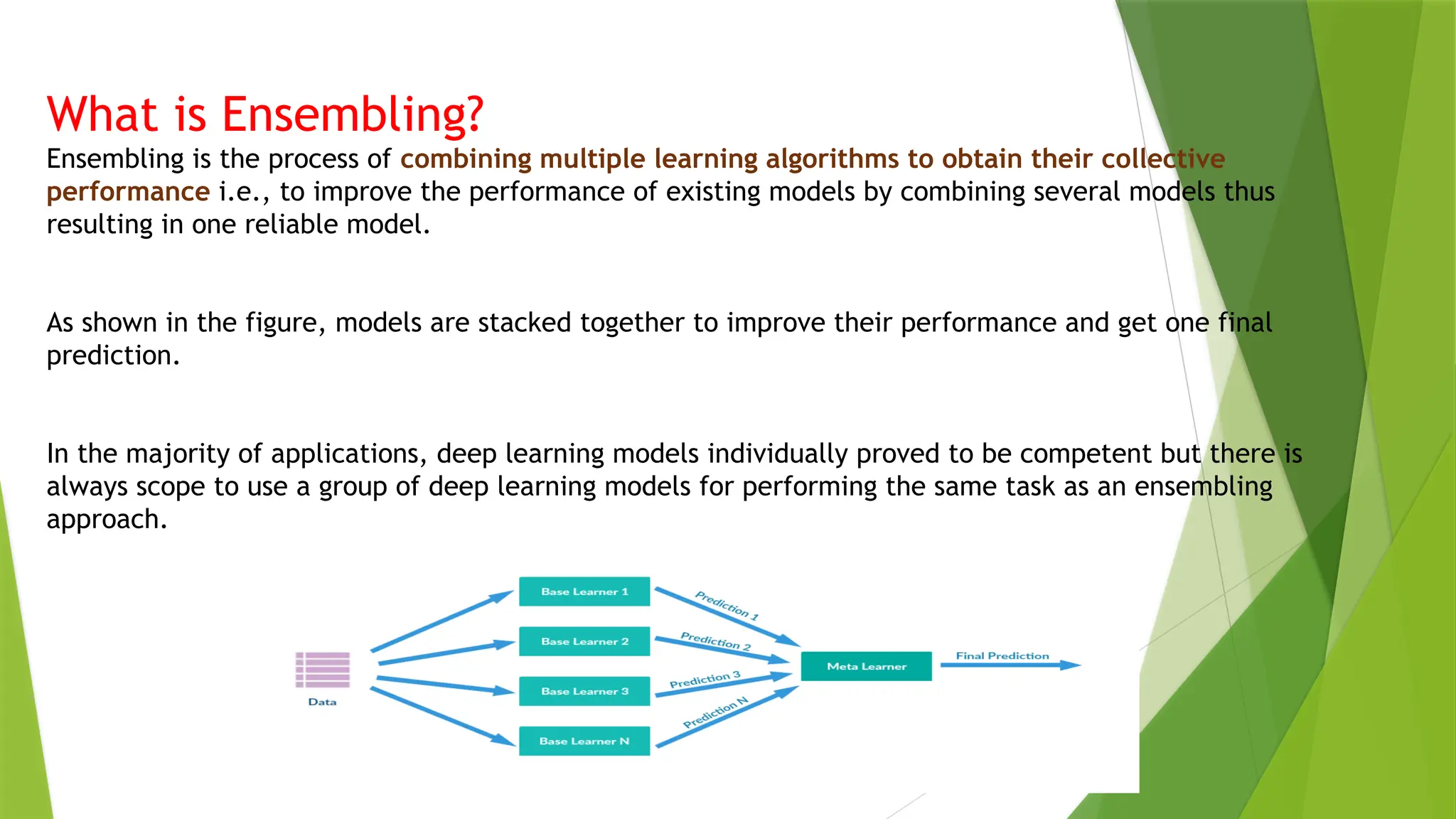
28. What is Ensembling?
Ensembling is the process of combining multiple learning algorithms to obtain their collective
performance i.e., to improve the performance of existing models by combining several models thus
resulting in one reliable model.
As shown in the figure, models are stacked together to improve their performance and get one final
prediction.
In the majority of applications, deep learning models individually proved to be competent but there is
always scope to use a group of deep learning models for performing the same task as an ensembling
approach.

29. What is bagging?
Bagging, also known as bootstrap aggregation, is the ensemble learning method that is commonly used to
reduce variance within a noisy dataset. In bagging,
a random sample of data in a training set is selected with replacement—meaning that the individual data
points can be chosen more than once.
After several data samples are generated, these weak models are then trained independently, and depending
on the type of task—regression or classification, for example—the average or majority of those predictions
yield a more accurate estimate.
Boosting ensemble method
Boosting creates an ensemble model by combining several weak decision trees sequentially. It assigns weights to
the output of individual trees. Then it gives incorrect classifications from the first decision tree a higher weight
and input to the next tree. After numerous cycles, the boosting method combines these weak rules into a single
powerful prediction rule.
Boosting compared to bagging
Boosting and bagging are the two common ensemble methods that improve prediction accuracy. The main
difference between these learning methods is the method of training. In bagging, data scientists improve the
accuracy of weak learners by training several of them at once on multiple datasets. In contrast, boosting trains

30. Bootstrapping
In statistics and machine learning, bootstrapping is a resampling technique that involves repeatedly drawing
samples from our source data with replacement, often to estimate a population parameter.
By “with replacement”, we mean that the same data point may be included in our resampled dataset multiple
times.
The term originates from the impossible idea of lifting ourselves up without external help, by pulling on our own
bootstraps.
Side note, but apparently it’s also why we “boot” up a computer (to run software, software must first be run,
so we bootstrap).
Typically our source data is only a small sample of the ground truth. Bootstrapping is loosely based on the law of
large numbers,
which says that with enough data the empirical distribution will be a good approximation of the true
distribution.