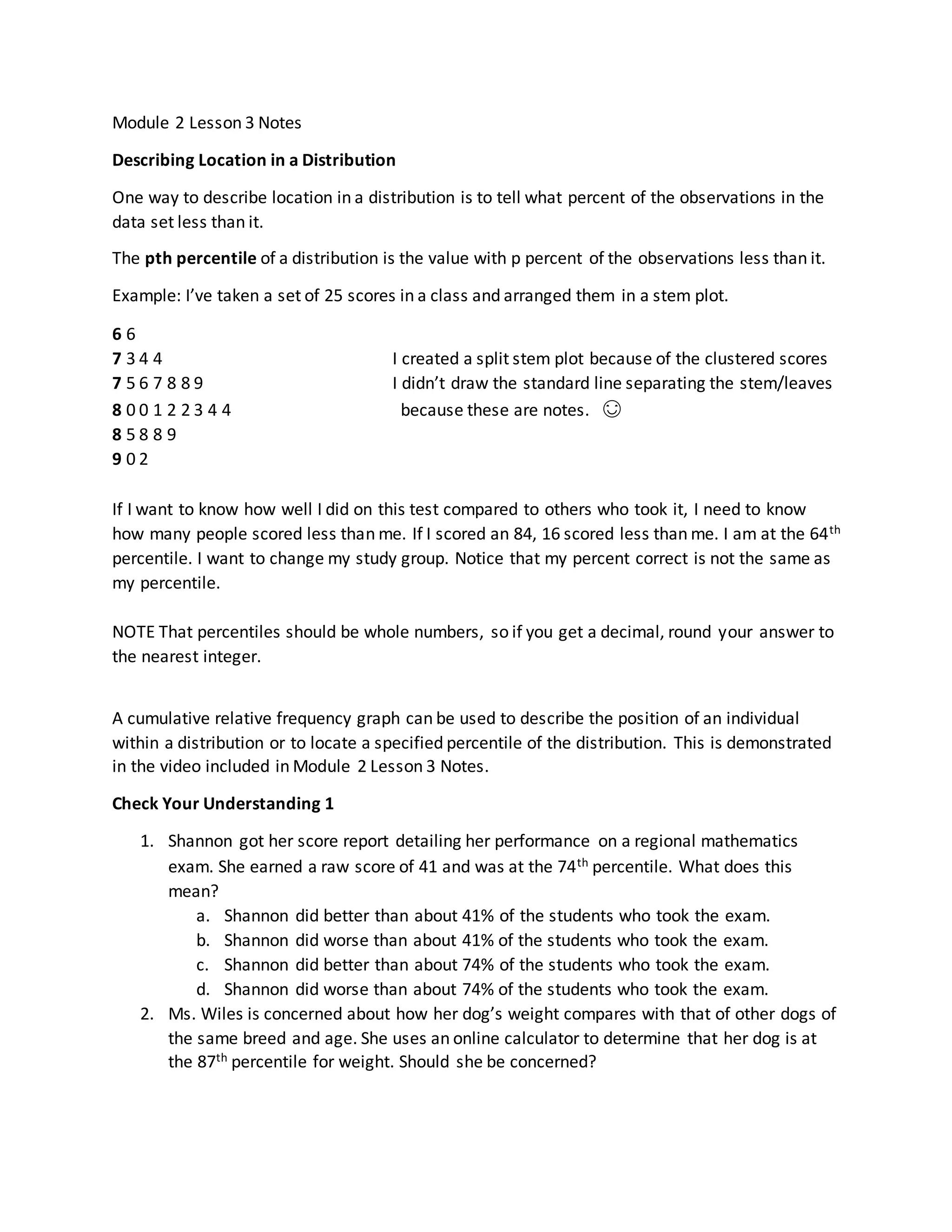
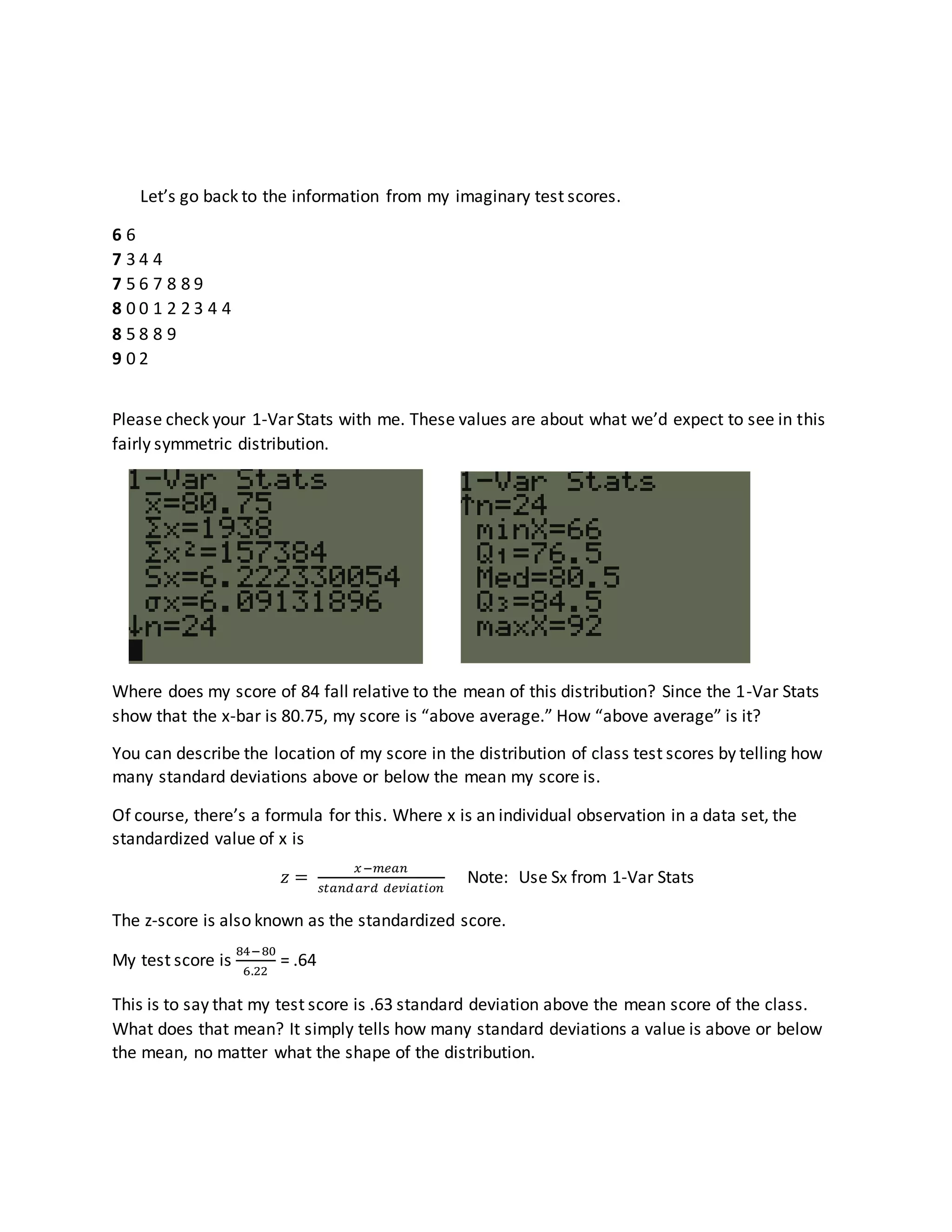
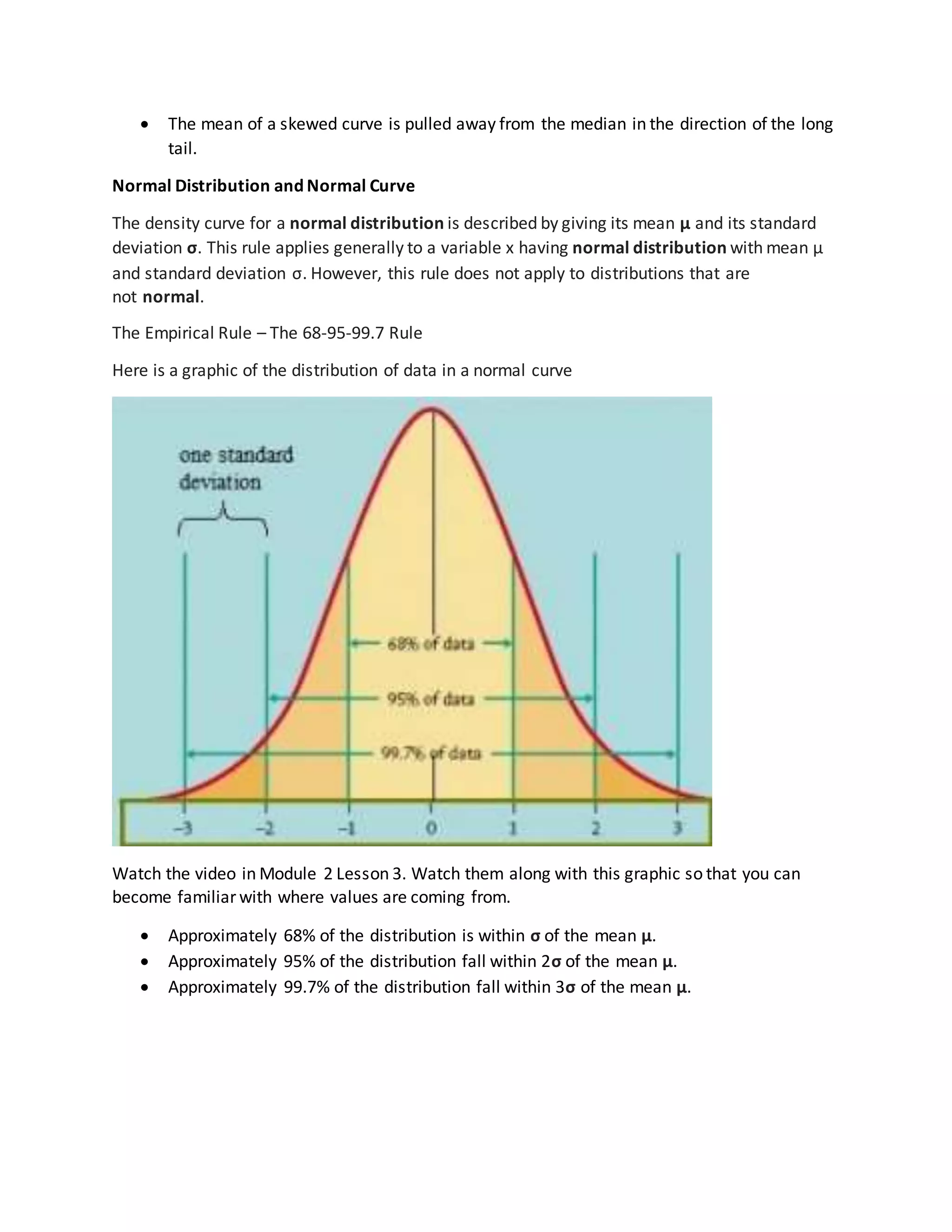
This document contains notes about describing location within a distribution. It discusses percentiles and how they describe the percentage of values below a given score. For example, the 64th percentile means 64% of scores were below that value. It also introduces z-scores as a way to standardize scores and compare values in different distributions based on their distance from the mean in units of standard deviation. Finally, it discusses density curves and how they can be used to describe an overall data pattern, with a normal distribution having 68% of values within 1 standard deviation of the mean.

1. Module 2 Lesson 3 Notes
Describing Location in a Distribution
One way to describe location in a distribution is to tell what percent of the observations in the
data set less than it.
The pth percentile of a distribution is the value with p percent of the observations less than it.
Example: I’ve taken a set of 25 scores in a class and arranged them in a stem plot.
6 6
7 3 4 4 I created a split stem plot because of the clustered scores
7 5 6 7 8 8 9 I didn’t draw the standard line separating the stem/leaves
8 0 0 1 2 2 3 4 4 because these are notes. 😊
8 5 8 8 9
9 0 2
If I want to know how well I did on this test compared to others who took it, I need to know
how many people scored less than me. If I scored an 84, 16 scored less than me. I am at the 64th
percentile. I want to change my study group. Notice that my percent correct is not the same as
my percentile.
NOTE That percentiles should be whole numbers, so if you get a decimal, round your answer to
the nearest integer.
A cumulative relative frequency graph can be used to describe the position of an individual
within a distribution or to locate a specified percentile of the distribution. This is demonstrated
in the video included in Module 2 Lesson 3 Notes.
Check Your Understanding 1
1. Shannon got her score report detailing her performance on a regional mathematics
exam. She earned a raw score of 41 and was at the 74th percentile. What does this
mean?
a. Shannon did better than about 41% of the students who took the exam.
b. Shannon did worse than about 41% of the students who took the exam.
c. Shannon did better than about 74% of the students who took the exam.
d. Shannon did worse than about 74% of the students who took the exam.
2. Ms. Wiles is concerned about how her dog’s weight compares with that of other dogs of
the same breed and age. She uses an online calculator to determine that her dog is at
the 87th percentile for weight. Should she be concerned?

2. Let’s go back to the information from my imaginary test scores.
6 6
7 3 4 4
7 5 6 7 8 8 9
8 0 0 1 2 2 3 4 4
8 5 8 8 9
9 0 2
Please check your 1-Var Stats with me. These values are about what we’d expect to see in this
fairly symmetric distribution.
Where does my score of 84 fall relative to the mean of this distribution? Since the 1-Var Stats
show that the x-bar is 80.75, my score is “above average.” How “above average” is it?
You can describe the location of my score in the distribution of class test scores by telling how
many standard deviations above or below the mean my score is.
Of course, there’s a formula for this. Where x is an individual observation in a data set, the
standardized value of x is
𝑧 =
𝑥−𝑚𝑒𝑎𝑛
𝑠𝑡𝑎𝑛𝑑𝑎𝑟𝑑 𝑑𝑒𝑣𝑖𝑎𝑡𝑖𝑜𝑛
Note: Use Sx from 1-Var Stats
The z-score is also known as the standardized score.
My test score is
84−80
6.22
= .64
This is to say that my test score is .63 standard deviation above the mean score of the class.
What does that mean? It simply tells how many standard deviations a value is above or below
the mean, no matter what the shape of the distribution.

3. We also use z-scores to compare the position of individuals in different distributions. I can use
z-scores to compare my performance on the ACT to the SAT or biology class to AP Stats class
even though they’re very different classes.
Many tests are standardized because test questions change from month to month but results
are used to compare over an extended time. Standardizing those results takes into accounts the
mean score of individual tests, along with the standard deviations to more equitably compare
tests that are not exactly the same.
Check Your Understanding 2
John is on the Varsity Basketball team. The mean height of the players on the team is 76 inches.
John’s height translates to a z-score of -0.85 in the team’s height distribution. What is the
standard deviation of the team members’ heights?
a. -2.35 inches
b. -2 inches
c. 2.35 inches
d. 2 inches
Density Curves
When exploring quantitative data
 Always plot your data – make a graph
o Dotplot
o Stemplot
o histogram
 Look for the overall pattern
 Calculate a numerical summary to describe center and spread
 SOMETIMES the pattern can be described by a smooth curve.
The density curve is not usually exactly symmetrical (normal) but does have these
characteristics:
 Always on or above the horizontal axis
 Has area exactly 1 (100%) underneath it
A density curve is a good description of the overall pattern of a distribution. No set of data is
exactly described nor are outliers determined though they may be hinted at. Areas under the
density curve represent proportions of the total number of observations.
 The median of the density curve is the equal areas point.
 The mean is the balance point.
 The mean and median of a symmetric density curve are the same.

4.  The mean of a skewed curve is pulled away from the median in the direction of the long
tail.
Normal Distribution and Normal Curve
The density curve for a normal distribution is described by giving its mean μ and its standard
deviation σ. This rule applies generally to a variable x having normal distribution with mean μ
and standard deviation σ. However, this rule does not apply to distributions that are
not normal.
The Empirical Rule – The 68-95-99.7 Rule
Here is a graphic of the distribution of data in a normal curve
Watch the video in Module 2 Lesson 3. Watch them along with this graphic so that you can
become familiar with where values are coming from.
 Approximately 68% of the distribution is within σ of the mean μ.
 Approximately 95% of the distribution fall within 2σ of the mean μ.
 Approximately 99.7% of the distribution fall within 3σ of the mean μ.

5. Check Your Understanding 3
Suppose that the distribution of batting averages is exactly normal with μ = 0.261and σ = 0.034.
NOTE: We write that as N(0.261, 0.034)
1. What percent of the batting averages are above 0.329?
2. What percent of the batting averages are between 0.193 and 0.295?
HINT: Sketch a Normal curves, label values then analyzing proportions.
Check Your Understanding 1 Answers
1. C
2. Ms. Wiles’ dog weighs more than about 87% of dogs of the same breed and age. She
should think about putting her dog on a healthy eating plan and perhaps visiting any
nearby doggy parks.
Check Your Understanding 2 Answer c
Check Your Understanding 3 Answers
1. About 2.5%
2. About 81.5%
Citation
Normal Curve Image http://www.statisticshowto.com/bell-curve/