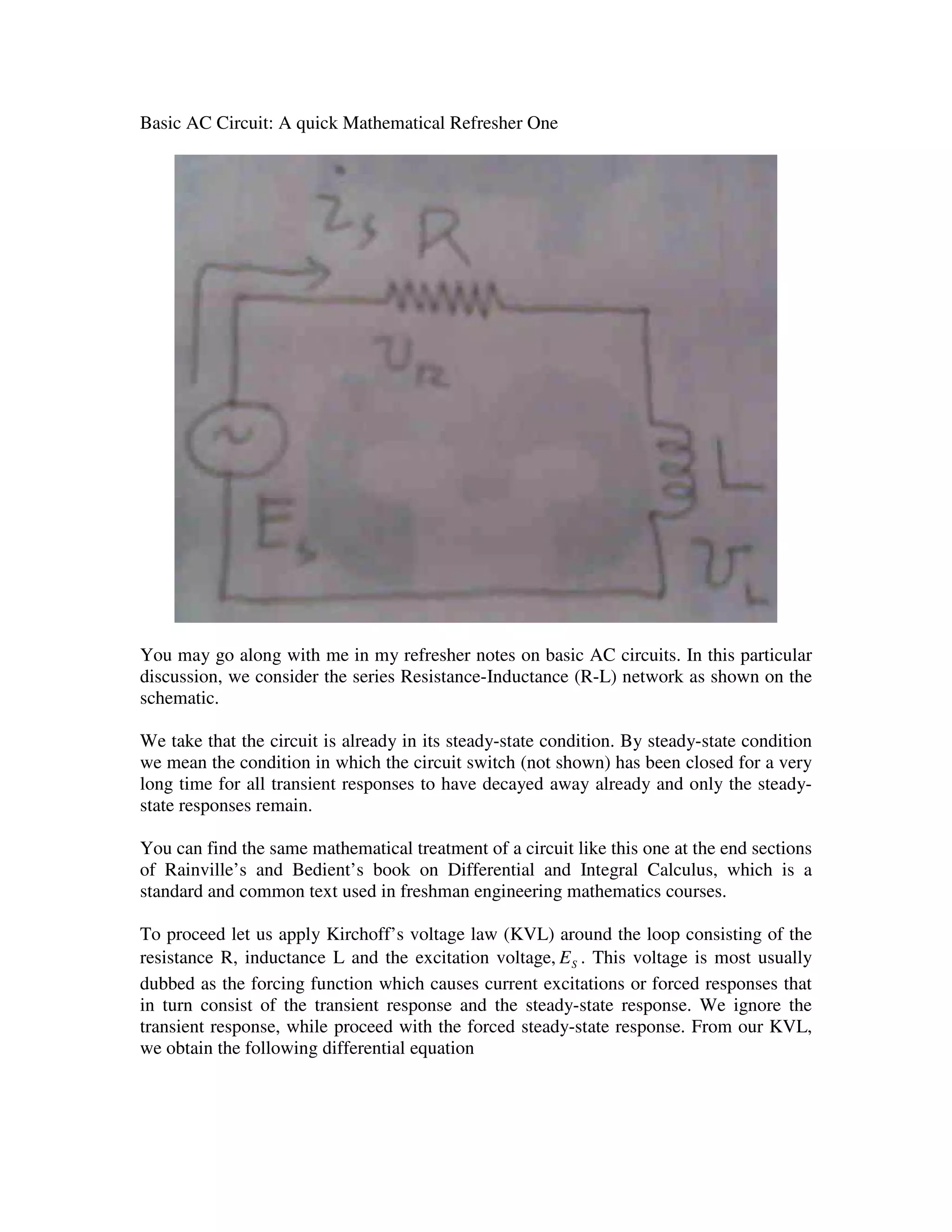
1) The document discusses the mathematical analysis of a basic AC circuit consisting of a resistor and inductor connected in series and driven by an external sinusoidal voltage source. 2) Kirchhoff's voltage law is applied to derive the differential equation governing the circuit and the forced steady-state response is shown to be a sinusoidal current lagging the driving voltage by a phase angle. 3) Expressions are derived relating the phase lag to the circuit properties and defining the real and reactive power consumed based on the circuit response.

1. Basic AC Circuit: A quick Mathematical Refresher One
You may go along with me in my refresher notes on basic AC circuits. In this particular
discussion, we consider the series Resistance-Inductance (R-L) network as shown on the
schematic.
We take that the circuit is already in its steady-state condition. By steady-state condition
we mean the condition in which the circuit switch (not shown) has been closed for a very
long time for all transient responses to have decayed away already and only the steady-
state responses remain.
You can find the same mathematical treatment of a circuit like this one at the end sections
of Rainville’s and Bedient’s book on Differential and Integral Calculus, which is a
standard and common text used in freshman engineering mathematics courses.
To proceed let us apply Kirchoff’s voltage law (KVL) around the loop consisting of the
resistance R, inductance L and the excitation voltage, SE . This voltage is most usually
dubbed as the forcing function which causes current excitations or forced responses that
in turn consist of the transient response and the steady-state response. We ignore the
transient response, while proceed with the forced steady-state response. From our KVL,
we obtain the following differential equation

2. (1)
L
E
i
L
R
dt
di S
=+
Because we assume that the circuit is already in its steady-state condition, we no longer
bother putting a unit-step function in (1) and that the current i is already in the steady-
state form.
For our circuit, let us give it, for example, a forcing function
(2)
tvE mSs ωsin−=
Given this forcing function, our resulting forced steady-state response would take the
following form
(3)
)(sin ψω −−== tiii mSS
Like the forcing function, this forced steady-state response is also a sinusoidal function of
time although this forced response lags the forcing function by a phase angleψ . This
forced response lags the forcing function by ψ since the forcing function attains its
maximum value mSEms vtE =)(ω first at
2
3π
ω =Emt , while the forced response has its
maximum mSimS iti =)(ω at a later while ψωω += Emim tt .
Our forced steady-state response satisfies the given D. E. (differential equation) provided
that the following relations hold
(4.1)
R
L
R
xL ω
ψ ==tan
(4.2)
22
sincos
L
L
xR
xR
z +===
ψψ

3. (4.3)
ziv mSmS =
(4.4)
mSmSmS vip =
(4.5)
Rip mSmS
2
cos =ψ real power
(4.6)
LmSmS xip
2
sin =ψ reactive power
Going around the loop once more to obtain the expression for instantaneous power as a
function of time
(5)
22
2
1
iL
dt
d
iRiEp SS +==
)2(cos
2
1
cos
2
1
ψωψ −−= tppp mSmSS
This, also in the steady-state condition, no longer includes the transient term. The
amplitude mSp
2
1
of the cosinusoidal oscillation in (5) can be determined from the root-
mean-square (rms) values of the forced steady-state response and the forcing function.
(6)
















==
22
)()(
2
1 mSmS
SSmS
vi
rmsErmsip
These rms values are the effective values of the forced steady-state response and the
forcing function and being effective values, they are directly read by measuring
instruments.

4. Over a time interval iF ttt −=∆ , we can calculate for example, the rms value of our
forcing function. This taken from an initial time it to a final time Ttt iF += . Here, T is
the period of one oscillation such that it satisfies the relation πω 2=T .
(7.1)
∫
+
=
∆
=
Tt
t
mS
SS
i
i
v
Etd
t
rmsE
2
1
)(
2
22
2
)( mS
S
v
rmsE =
Let us note here the result
(7.2)
∫
+
=
Tt
t
i
i
tdt 02cos ω
Likewise
(7.3)
∫
+
=
∆
=
Tt
t
mS
SS
i
i
i
itd
t
rmsi
2
1
)(
2
22
2
)( mS
S
i
rmsi =
Also here,
(7.4)
∫
+
=−
Tt
t
i
i
tdt 0)2(cos ψω
Analogously, we apply this same way of obtaining rms values in getting for the rms value
of power over the same time interval and initial and final time boundaries.
(8.1)
∫
+
∆
=
Tt
t
SS
i
i
ptd
t
rmsp 22 1
)(

5. 





+= mSS prmsp
2
1
cos
2
1
)( 2
ψ
Also to be noted here,
(8.2)
∫
+
=−
Tt
t
i
i
tndt 0)22(sin ψω
(8.3)
∫
+
=−
Tt
t
i
i
tndt 0)22(cos ψω
where n is all integer excluding zero.
We can write the square of (8.1) as a sum of two squares,
(9.1)
)(
2
1
2
1
)( 2
2
2
avpprmsp SmsS +





=
Here, the average value of power is obtained by
(9.2)
ψcos
2
11
)( mS
Tt
t
SS pptd
t
avp
i
i
=
∆
= ∫
+
Notice that this average value of power is dependent on the cosine of the phase angle.
This average value is zero for a purely inductive circuit in which the phase angle is
90degrees, while this value is greatest for a purely resistive circuit with a phase angle of
zero degree. From this we see that the contribution of this average value to the rms value
of power is greatest for a purely resistive circuit. Let us note that the average value of
power is half of the real power in (4.5) and represented by the constant part in the
instantaneous value of power at time t given by (5). From this instantaneous value of
power given at time t we can obtain for the instantaneous value of energy expended at
time t.

6. (10.1)
( ) SmSmSS ctptp +−−= )2(sin
4
1
cos
2
1
ψω
ω
ψε
Let’s be reminded that we are still ignoring the transient parts. In this expression, we
have included a constant of integration Sc and the average value of power enters this
expression in a term linear in time t. Say we have a given t which is an integral multiple
of the period T so that we may write (10.1) as
(10.2)
( ) ( ) SLmSS cNTpTNt +





+== τψε
2
1
)(cos
2
1
The constant Lτ is the reciprocal of the time-constant LRL /1
=−
τ and this is a constant
involved in an exponential factor if we have included the transient term containing this
factor
(10.3)
( )Lt τ/exp −
We can have the approximation that for all LTN τ
2
1
>> , (10.2) reduces to
(10.4)
( ) ( ) SmSS cTNpTNt +≈= )(cos
2
1
ψε
So at this instant and up to some additive constant, the value of instantaneous energy
expended is dominated by the term that contains the average value of power. Recall that
this average value is half of the real power. Take note that for all lower values of
inductance L for a given frequency Tf /1= , the linear part in (10.1) dominates more
quickly over sinusoidal oscillation with transient term ignored. Here, the circuit behaves
more of a resistive load expending more energy quickly.