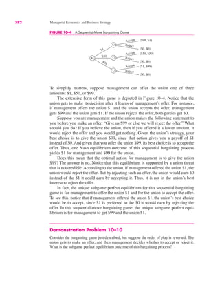
This document provides the table of contents for the 7th edition of the textbook "Managerial Economics and Business Strategy" by Michael R. Baye. The summary highlights that the textbook covers a wide range of microeconomic concepts and business strategies including Nash equilibrium, demand elasticity, marginal cost, learning curves, repeated games, antitrust, price discrimination, auctions, and more. It is intended to provide students with the tools from intermediate microeconomics, game theory, and industrial organization to make sound managerial decisions. The textbook includes real-world examples, applications, and a case study on challenges at Time Warner corporation. It aims to be flexible for instructors to tailor to their specific course needs.


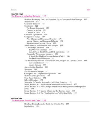
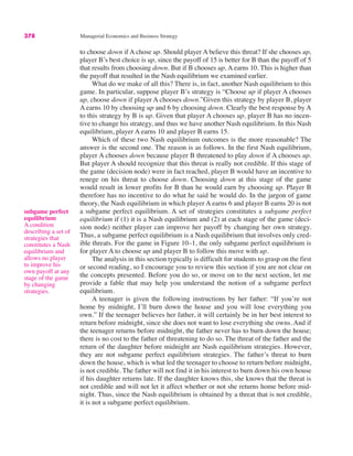
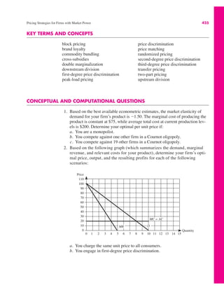
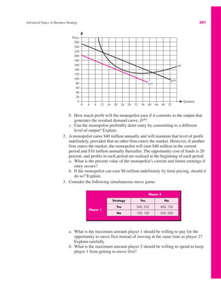
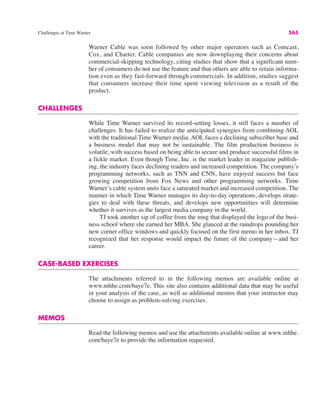
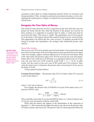
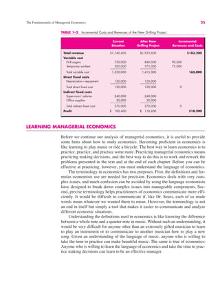
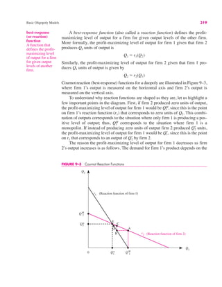
![Amcott Loses $3.5 Million;
Manager Fired
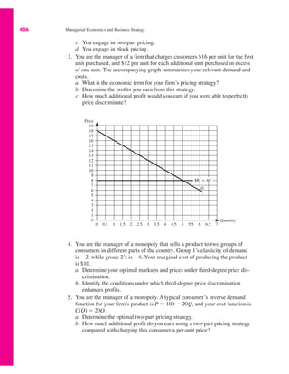
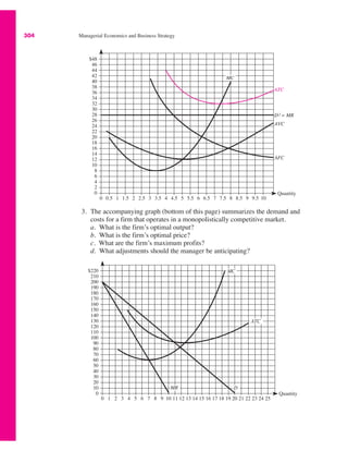
On Tuesday software giant Amcott posted a year-end
operating loss of $3.5 million. Reportedly, $1.7 mil-
lion of the loss stemmed from its foreign language
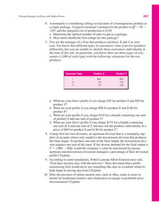
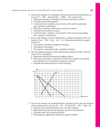
division.
With short-term interest rates at 7 percent,
Amcott decided to use $20 million of its retained
earnings to purchase three-year rights to Magicword,
a software package that converts generic word proces-
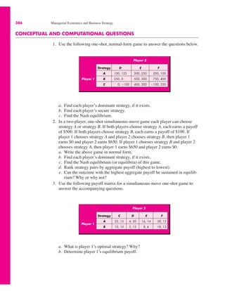
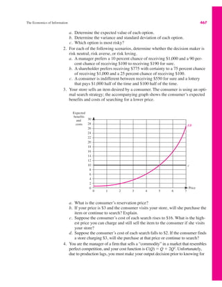
sor files saved as French text into English. First-year
sales revenue from the software was $7 million, but
thereafter sales were halted pending a copyright
infringement suit filed by Foreign, Inc. Amcott lost
the suit and paid damages of $1.7 million. Industry
insiders say that the copyright violation pertained to
“a very small component of Magicword.”
Ralph, the Amcott manager who was fired over the
incident, was quoted as saying, “I’m a scapegoat for
the attorneys [at Amcott] who didn’t do their home-
work before buying the rights to Magicword. I pro-
jected annual sales of $7 million per year for three years. My sales forecasts were right on target.”
Do you know why Ralph was fired?1
CHAPTER
ONE
HEADLINE
The Fundamentals of
Managerial Economics
1
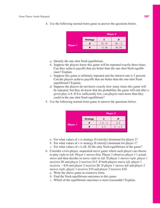
1
Each chapter concludes with an answer to the question posed in that chapter's
opening headline. After you read each chapter, you should attempt to solve the opening
headline on your own and then compare your solution to that presented at the end of
the chapter.
Learning Objectives
After completing this chapter, you will be
able to:
LO1 Summarize how goals, constraints, incen-
tives, and market rivalry affect economic
decisions.
LO2 Distinguish economic versus accounting
profits and costs.
LO3 Explain the role of profits in a market
economy.
LO4 Apply the five forces framework to analyze
the sustainability of an industry’s profits.
LO5 Apply present value analysis to make
decisions and value assets.
LO6 Apply marginal analysis to determine
the optimal level of a managerial control
variable.
LO7 Identify and apply six principles of effec-
tive managerial decision making.](https://image.slidesharecdn.com/managerialeconomicsmichaelbaye2-230815092539-2513f09d/85/Managerial_economics_michael_baye-2-pdf-34-320.jpg)
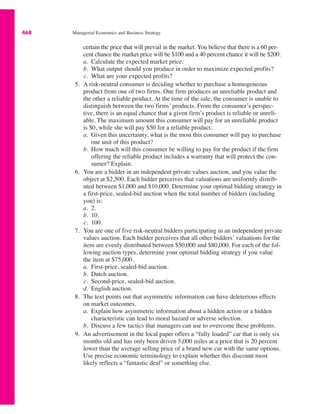
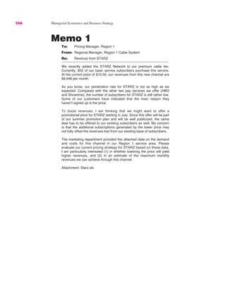
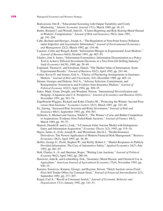
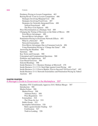
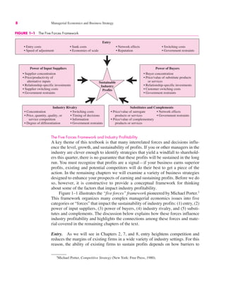
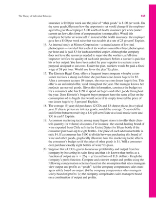
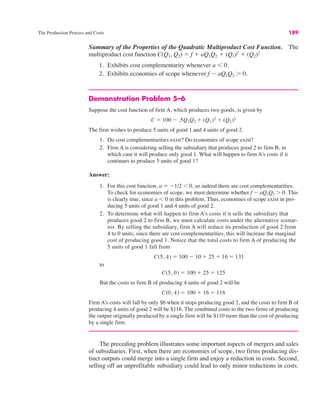
![INSIDE BUSINESS 1–1
The Goals of Firms in Our Global Economy
Recent trends in globalization have forced businesses
around the world to more keenly focus on profitability.
This trend is also present in Japan, where historical
links between banks and businesses have traditionally
blurred the goals of firms. For example, the Japanese
business engineering firm, Mitsui & Co. Ltd., recently
launched “Challenge 21,” a plan directed at helping
the company emerge as Japan’s leading business engi-
neering group. According to a spokesperson for the
company, “[This plan permits us to] create new value
and maximize profitability by taking steps such as
renewing our management framework and prioritizing
the allocation of our resources into strategic areas. We
are committed to maximizing shareholder value
through business conduct that balances the pursuit of
earnings with socially responsible behavior.”
Ultimately, the goal of any continuing company
must be to maximize the value of the firm. This goal is
often achieved by trying to hit intermediate targets, such
as minimizing costs or increasing market share. If you—
as a manager—do not maximize your firm’s value over
time, you will be in danger of either going out of busi-
ness, being taken over by other owners (as in a leveraged
buyout), or having stockholders elect to replace you and
other managers.
Source: “Mitsui & Co., Ltd. UK Regulatory
Announcement: Final Results,” Business Wire,
May 13, 2004.
The Fundamentals of Managerial Economics 7
Smith is saying that by pursuing its self-interest—the goal of maximizing
profits—a firm ultimately meets the needs of society. If you cannot make a living
as a rock singer, it is probably because society does not appreciate your singing;
society would more highly value your talents in some other employment. If you
break five dishes each time you clean up after dinner, your talents are perhaps
better suited for balancing the checkbook or mowing the lawn. Similarly, the
profits of businesses signal where society’s scarce resources are best allocated.
When firms in a given industry earn economic profits, the opportunity cost to
resource holders outside the industry increases. Owners of other resources soon
recognize that, by continuing to operate their existing businesses, they are giving
up profits. This induces new firms to enter the markets in which economic profits
are available. As more firms enter the industry, the market price falls, and eco-
nomic profits decline.
Thus, profits signal the owners of resources where the resources are most
highly valued by society. By moving scarce resources toward the production of
goods most valued by society, the total welfare of society is improved. As Adam
Smith first noted, this phenomenon is due not to benevolence on the part of the
firms’ managers but to the self-interested goal of maximizing the firms’ profits.
Principle Profits Are a Signal
Profits signal to resource holders where resources are most highly valued by society.](https://image.slidesharecdn.com/managerialeconomicsmichaelbaye2-230815092539-2513f09d/85/Managerial_economics_michael_baye-2-pdf-40-320.jpg)
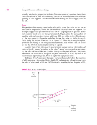
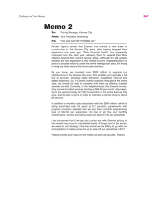
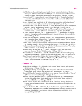
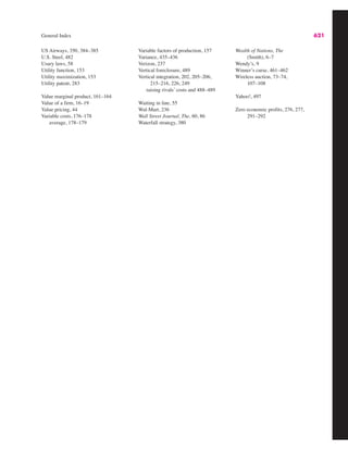
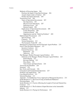
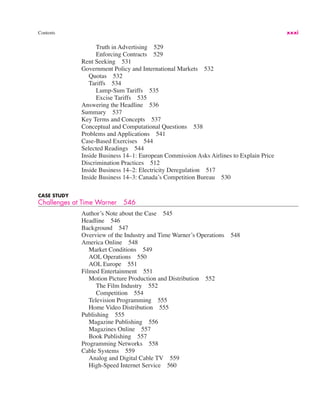
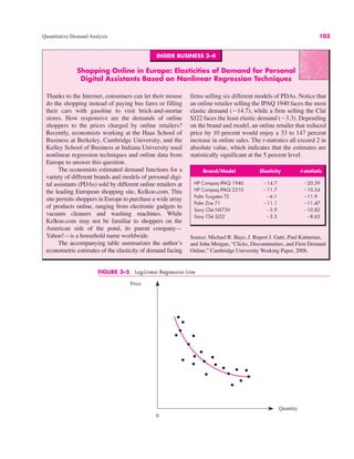
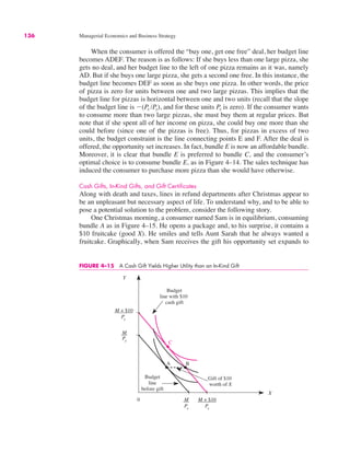
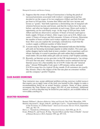
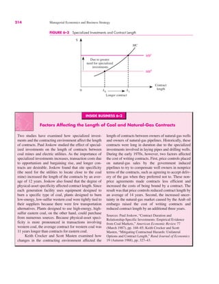
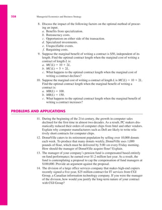
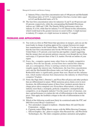
![INSIDE BUSINESS 3–3
Using Cross-Price Elasticities to Improve New Car Sales in the
Wake of Increasing Gasoline Prices
At the close of the last century, increases in the price of
gasoline led to decreases in demand for products that
are complements for gasoline, such as automobiles. The
reason was that higher gasoline prices moved con-
sumers to substitute toward public transportation, bicy-
cling, and walking. An econometric study by Patrick
McCarthy provides quantitative information about the
impact of fuel costs on the demand for automobiles.
One of the more important determinants of the demand
for automobiles is the fuel operating cost, defined as the
cost of fuel per mile driven. The study reveals that for
each 1 percent increase in fuel costs, the demand for
automobiles will decrease by 0.214 percent. A 10 per-
cent increase in the price of gasoline increases the cost
of fuel per mile driven by 10 percent and thus reduces
the demand for a given car by 2.14 percent.
What did automakers do during this period to
mitigate the negative impact of rising gasoline
prices on the demand for new automobiles? They
made cars more fuel efficient. The results just sum-
marized imply that for every 10 percent increase in
fuel efficiency (measured by the increase in miles
per gallon), the demand for automobiles increases
by 2.14 percent. Auto manufacturers could com-
pletely offset the negative impact of higher gasoline
prices by increasing the fuel efficiency of new cars
by the same percentage as the increase in gasoline
prices. In fact, by increasing fuel efficiency by a
greater percentage than the increase in gasoline
prices, they would actually increase the demand for
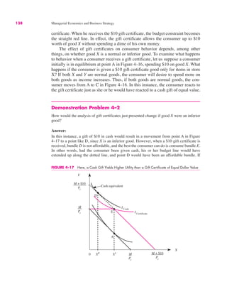
new automobiles.
Source: Patrick S. McCarthy, “Consumer Demand for
Vehicle Safety: An Empirical Study,” Economic Inquiry 28
(July 1990), pp. 530–43.
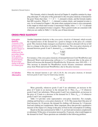
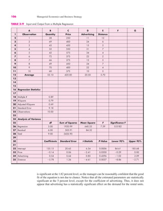
Quantitative Demand Analysis 87
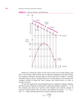
More generally, suppose a firm’s revenues are derived from the sales of two
products, X and Y. We may express the firm’s revenues as R ! Rx # Ry, where Rx !
PxQx denotes revenues from the sale of product X and Ry ! PyQy represents rev-
enues from product Y. The impact of a small percentage change in the price of
product X (%$Px ! $Px/Px) on the total revenues of the firm is1
To illustrate how to use this formula, suppose a restaurant earns $4,000 per
week in revenues from hamburger sales (product X) and $2,000 per week from soda
sales (product Y). Thus, Rx ! $4,000 and Ry ! $2,000. If the own price elasticity of
demand for burgers is and the cross-price elasticity of demand
between sodas and hamburgers is what would happen to the firm’s
total revenues if it reduced the price of hamburgers by 1 percent? Plugging these
numbers into the above formula reveals
EQy, Px
! "4.0,
EQx, Px
! "1.5
$R ! [Rx(1 # EQx, P
x
) # RyEQy, Px
] ) %$Px
1
This formula is an approximation for large changes in price.](https://image.slidesharecdn.com/managerialeconomicsmichaelbaye2-230815092539-2513f09d/85/Managerial_economics_michael_baye-2-pdf-120-320.jpg)

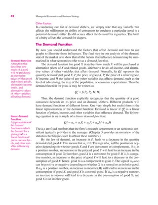
income elasticity
A measure of the
responsiveness of
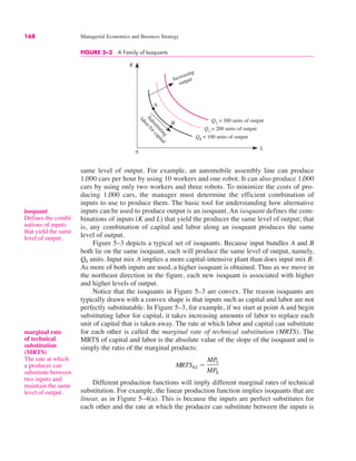
the demand for a
good to changes in
consumer income;
the percentage
change in quantity
demanded divided
by the percentage
change in income.
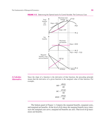
A Calculus
Alternative
The income elasticity for a good with a demand function may be found
using calculus:
EQx, M !
%Qx
d
%M
M
Qx
Qx
d ! f(P
x, Py, M, H)
When good X is a normal good, an increase in income leads to an increase in
the consumption of X. Thus, when X is a normal good. When X is an infe-
rior good, an increase in income leads to a decrease in the consumption of X. Thus,
when X is an inferior good.
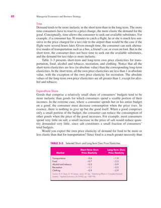
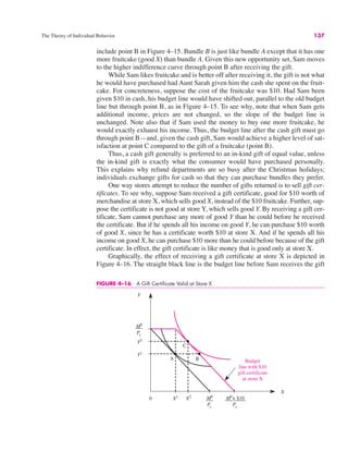
Table 3–5 presents some recent estimates of income elasticities for various
products. Consider, for example, the income elasticity for transportation, 1.8. This
number gives us two important pieces of information about the relationship
between income and the demand for transportation. First, since the income elastic-
ity is positive, we know that consumers increase the amount they spend on trans-
portation when their incomes rise. Transportation thus is a normal good. Second,
since the income elasticity for transportation is greater than 1, we know that expen-
ditures on transportation grow more rapidly than income.
The second row of Table 3–5 reveals that food also is a normal good, since the
income elasticity of food is 0.8. Since the income elasticity is less than 1, an increase
in income will increase the expenditure on food by a lower percentage than the
EQx, M & 0
EQx, M ' 0](https://image.slidesharecdn.com/managerialeconomicsmichaelbaye2-230815092539-2513f09d/85/Managerial_economics_michael_baye-2-pdf-121-320.jpg)
![104 Managerial Economics and Business Strategy
To estimate a log-linear demand function, the econometrician takes the natural
logarithm of prices and quantities before executing the regression routine that min-
imizes the sum of squared errors (e):
In other words, by using a spreadsheet to compute Q- ! ln Q and P- ! ln P, this
demand specification can be viewed equivalently as
which is linear in Q- and P-. Therefore, one can use procedures identical to those
described earlier and regress the transformed Q- on P- to obtain parameter esti-
mates. Recall that the resulting parameter estimate for bP in this case is the own
price elasticity of demand, since this is a log-linear demand function.
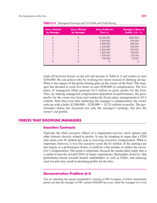
Demonstration Problem 3–5
During the 31 days this past March, an online ticket agent offered varying price discounts on
Broadway tickets in order to gather information needed to estimate the demand for its tick-
ets. A file named Demo_3_5.xls is available online at www.mhhe.com/baye7e. If you open
this file and view the tab labeled Data, you will find information about the quantity of
Broadway tickets the company sold at various prices in March. Use these data to estimate a
log-linear demand function. Use an equation to summarize your findings.
Answer:
The first step is to transform the price and quantity data into natural logarithms, using the
relevant spreadsheet command. You can see how to do this step by viewing the tab labeled
Transformed in the Demo_3_5.xls file. The second step is to perform a linear regression on
the transformed data. These regression results are displayed in the Results tab of the file. The
final step is to summarize the regression results in a demand equation. In this case, the esti-
mates in the Results tab imply the following log-linear demand function:
Written in this manner, the logarithm of quantity demanded is a linear function of the
logarithm of price, and the company’s elasticity of demand for tickets is "1.58. Alterna-
tively, one can express the actual quantity demanded as a nonlinear function of price by tak-
ing the exponential of both sides of the above equation:
Multiple Regression
In general, the demand for a good will depend not only on the good’s price, but
also on demand shifters. Regression techniques can also be used to perform mul-
tiple regressions—regressions of a dependent variable on multiple explanatory
Qd ! 4629P"1.58
Qd ! exp [8.44]P"1.58
exp[ln Qd] ! exp[8.44] exp[ "1.58 ln P]
ln Qd ! 8.44 " 1.58 ln P
Q- ! b0 # bPP- # e
ln Q ! b0 # bP ln P # e](https://image.slidesharecdn.com/managerialeconomicsmichaelbaye2-230815092539-2513f09d/85/Managerial_economics_michael_baye-2-pdf-137-320.jpg)
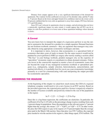
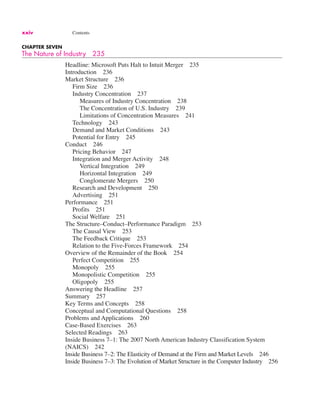
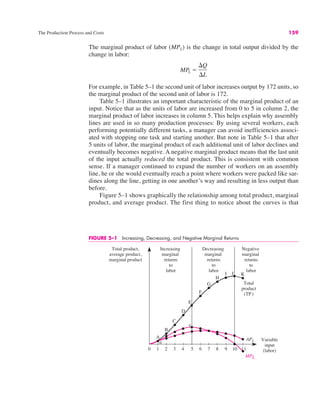
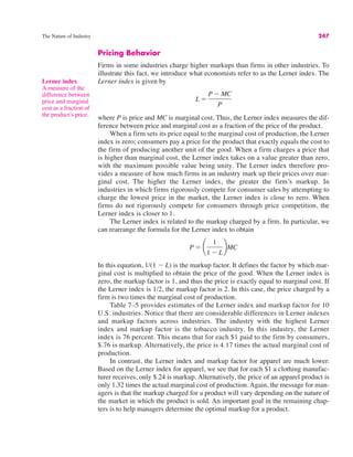
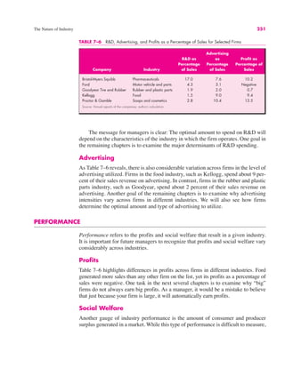
![The Production Process and Costs 157
TABLE 5–1 The Production Function
(1) (2) (3) (4) (5) (6)
K* L !L Q
Fixed Variable Change Output Marginal Average
Input Input in Product Product
(Capital) (Labor) Labor of Labor of Labor
[Given] [Given] [!(2)] [Given] [!(4)/!(2)] [(4)/(2)]
2 0 — 0 — —
2 1 1 76 76 76
2 2 1 248 172 124
2 3 1 492 244 164
2 4 1 784 292 196
2 5 1 1,100 316 220
2 6 1 1,416 316 236
2 7 1 1,708 292 244
2 8 1 1,952 244 244
2 9 1 2,124 172 236
2 10 1 2,200 76 220
2 11 1 2,156 "44 196
Q
L
" APL
!Q
!L
" MPL
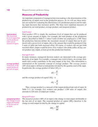
making input decisions. For example, it takes several years for automakers to
develop and build new assembly lines for producing hybrids. The level of capital is
generally fixed in the short run. However, in the short run automakers can adjust
their use of inputs such as labor and steel; such inputs are called variable factors of
production.
The short run is defined as the time frame in which there are fixed factors of
production. To illustrate, suppose capital and labor are the only two inputs in pro-
duction and that the level of capital is fixed in the short run. In this case the only
short-run input decision to be made by a manager is how much labor to utilize. The
short-run production function is essentially only a function of labor, since capital is
fixed rather than variable. If K* is the fixed level of capital, the short-run produc-
tion function may be written as
Columns 1, 2, and 4 in Table 5–1 give values of the components of a short-run
production function where capital is fixed at K* ! 2. For this production function,
5 units of labor are needed to produce 1,100 units of output. Given the available
technology and the fixed level of capital, if the manager wishes to produce
1,952 units of output, 8 units of labor must be utilized. In the short run, more labor
is needed to produce more output, because increasing capital is not possible.
The long run is defined as the horizon over which the manager can adjust all
factors of production. If it takes a company three years to acquire additional capital
machines, the long run for its management is three years, and the short run is less
than three years.
Q ! f(L) ! F(K*, L)
fixed and
variable factors
of production
Fixed factors are
the inputs the
manager cannot
adjust in the short
run. Variable
factors are the
inputs a manager
can adjust to alter
production.](https://image.slidesharecdn.com/managerialeconomicsmichaelbaye2-230815092539-2513f09d/85/Managerial_economics_michael_baye-2-pdf-190-320.jpg)
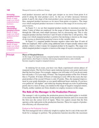
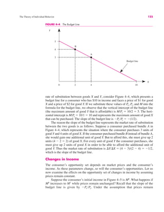
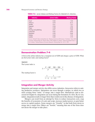
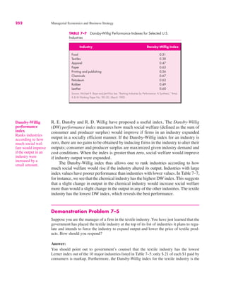
![162 Managerial Economics and Business Strategy
Principle Profit-Maximizing Input Usage
To maximize profits, a manager should use inputs at levels at which the marginal benefit
equals the marginal cost. More specifically, when the cost of each additional unit of labor
is w, the manager should continue to employ labor up to the point where VMPL ! w in the
range of diminishing marginal product.
TABLE 5–2 The Value Marginal Product of Labor
(1) (2) (3) (4) (5)
L P VMPL " P # MPL W
Marginal
Variable Price Product Value Marginal Unit Cost
Input of of Labor Product of
(Labor) Output [Column 5 of of Labor Labor
[Given] [Given] Table 5–1] [(2) # (3)] [Given]
0 $3 — — $400
1 3 76 $228 400
2 3 172 516 400
3 3 244 732 400
4 3 292 876 400
5 3 316 948 400
6 3 316 948 400
7 3 292 876 400
8 3 244 732 400
9 3 172 516 400
10 3 76 228 400
11 3 "44 "132 400
!Q
!L
" MPL
The profit-maximizing input usage rule defines the demand for an input by a
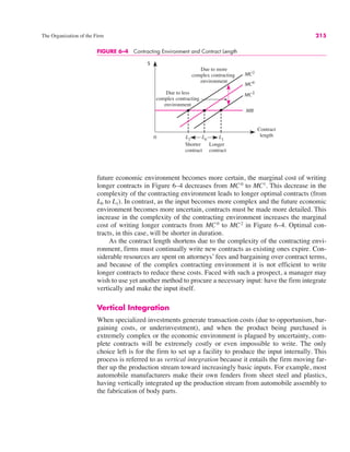
profit-maximizing firm. For example, in Figure 5–2 the value marginal product of
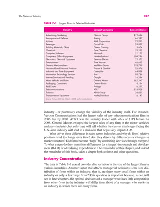
labor is graphed as a function of the quantity of labor utilized. When the wage rate
FIGURE 5–2 The Demand for Labor
0
w
L
L0
w0
Profit-
maximizing
point
VMPL
Demand
for labor](https://image.slidesharecdn.com/managerialeconomicsmichaelbaye2-230815092539-2513f09d/85/Managerial_economics_michael_baye-2-pdf-195-320.jpg)
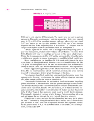
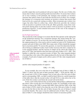
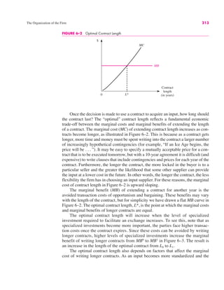
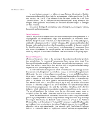
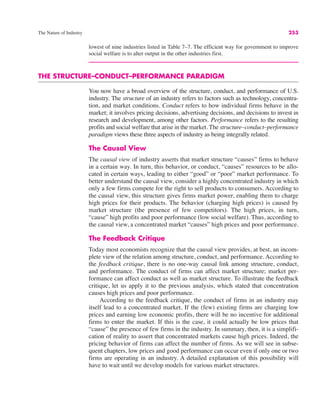
![The Production Process and Costs 177
short-run cost function summarizes the minimum possible cost of producing each
level of output when variable factors are being used in the cost-minimizing way.
Table 5–3 illustrates the costs of producing with the technology used in Table
5–1. Notice that the first three columns comprise a short-run production function
because they summarize the maximum amount of output that can be produced with
two units of the fixed factor (capital) and alternative units of the variable factor
(labor). Assuming capital costs $1,000 per unit and labor costs $400 per unit, we
can calculate the fixed and variable costs of production, which are summarized in
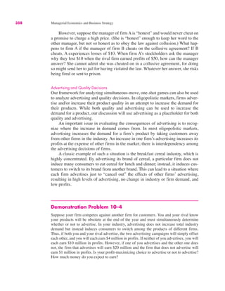
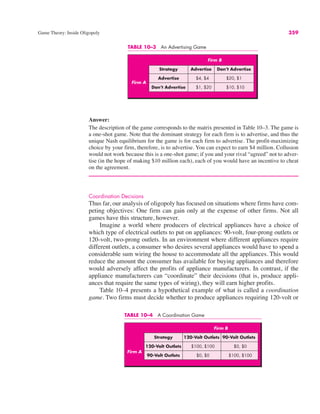
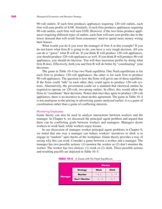
columns 4 and 5 of Table 5–3. Notice that irrespective of the amount of output pro-
duced, the cost of the capital equipment is $1,000 $ 2 ! $2,000. Thus, every entry
in column 4 contains this number, illustrating the principle that fixed costs do not
vary with output.
To produce more output, more of the variable factor must be employed. For
example, to produce 1,100 units of output, 5 units of labor are needed; to produce
1,708 units of output, 7 units of labor are required. Since labor is the only variable
input in this simple example, the variable cost of producing 1,100 units of output is
the cost of 5 units of labor, or $400 $ 5 ! $2,000. Similarly, the variable cost of
producing 1,708 units of output is $400 $ 7 ! $2,800. Total costs, summarized in
the last column of Table 5–3, are simply the sum of fixed costs (column 4) and vari-
able costs (column 5) at each level of output.
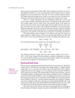
Figure 5–11 illustrates graphically the relations among total costs (TC), vari-
able costs (VC), and fixed costs (FC). Because fixed costs do not change with out-
put, they are constant for all output levels and must be paid even if zero units of
output are produced. Variable costs, on the other hand, are zero if no output is pro-
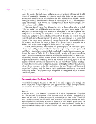
duced but increase as output increases above zero. Total cost is the sum of fixed
TABLE 5–3 The Cost Function
(1) (2) (3) (4) (5) (6)
K L Q FC VC TC
Fixed Variable Output Fixed Variable Total
Input Input Cost Cost Cost
[Given] [Given] [Given] [$1,000 # (1)] [$400 # (2)] [(4) $ (5)]
2 0 0 $2,000 $ 0 $2,000
2 1 76 2,000 400 2,400
2 2 248 2,000 800 2,800
2 3 492 2,000 1,200 3,200
2 4 784 2,000 1,600 3,600
2 5 1,100 2,000 2,000 4,000
2 6 1,416 2,000 2,400 4,400
2 7 1,708 2,000 2,800 4,800
2 8 1,952 2,000 3,200 5,200
2 9 2,124 2,000 3,600 5,600
2 10 2,200 2,000 4,000 6,000
short-run cost
function
A function that
defines the mini-
mum possible cost
of producing each
output level when
variable factors are
employed in the
cost-minimizing
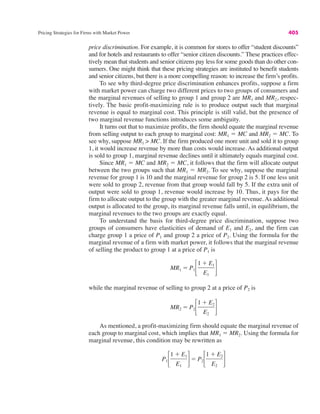
fashion.](https://image.slidesharecdn.com/managerialeconomicsmichaelbaye2-230815092539-2513f09d/85/Managerial_economics_michael_baye-2-pdf-210-320.jpg)
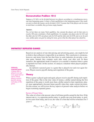
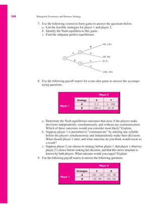
![The Production Process and Costs 179
Column 6 of Table 5–4 provides the average variable cost for the production func-
tion in our example. Notice that as output increases, average variable cost initially
declines, reaches a minimum between 1,708 and 1,952 units of output, and then
begins to increase.
Average total cost is analogous to average variable cost, except that it provides
a measure of total costs on a per-unit basis. Average total cost (ATC) is defined as
total cost (TC) divided by the number of units of output:
Column 7 of Table 5–4 provides the average total cost of various outputs in our
example. Notice that average total cost declines as output expands to 2,124 units and
then begins to rise. Furthermore, note that average total cost is the sum of average
fixed costs and average variable costs (the sum of columns 5 and 6) in Table 5–4.
The most important cost concept is marginal (or incremental) cost. Conceptu-
ally, marginal cost (MC) is the cost of producing an additional unit of output, that
is, the change in cost attributable to the last unit of output:
To understand this important concept, consider Table 5–5, which summarizes
the short-run cost function with which we have been working. Marginal cost,
depicted in column 7, is calculated as the change in costs arising from a given
change in output. For example, increasing output from 248 to 492 units (#Q ! 244)
increases costs from 2,800 to 3,200 (#C ! $400). Thus, the marginal cost of
increasing output to 492 units is #C/#Q ! 400/244 ! $1.64.
MC !
#C
#Q
ATC !
C(Q)
Q
TABLE 5–4 Derivation of Average Costs
(1) (2) (3) (4) (5) (6) (7)
Q FC VC TC AFC AVC ATC
Output Fixed Variable Total Average Average Average
Cost Cost Cost Fixed Variable Total
Cost Cost Cost
[Given] [Given] [Given] [(2) $ (3)] [(2)/(1)] [(3)/(1)] [(4)/(1)]
0 $2,000 $ 0 $2,000 — — —
76 2,000 400 2,400 $26.32 $5.26 $31.58
248 2,000 800 2,800 8.06 3.23 11.29
492 2,000 1,200 3,200 4.07 2.44 6.50
784 2,000 1,600 3,600 2.55 2.04 4.59
1,100 2,000 2,000 4,000 1.82 1.82 3.64
1,416 2,000 2,400 4,400 1.41 1.69 3.11
1,708 2,000 2,800 4,800 1.17 1.64 2.81
1,952 2,000 3,200 5,200 1.02 1.64 2.66
2,124 2,000 3,600 5,600 0.94 1.69 2.64
2,200 2,000 4,000 6,000 0.91 1.82 2.73
marginal
(incremental)
cost
The cost of produc-
ing an additional
unit of output.](https://image.slidesharecdn.com/managerialeconomicsmichaelbaye2-230815092539-2513f09d/85/Managerial_economics_michael_baye-2-pdf-212-320.jpg)
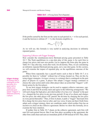
![180 Managerial Economics and Business Strategy
TABLE 5–5 Derivation of Marginal Costs
(1) (2) (3) (4) (5) (6) (7)
Q ! Q VC ! VC TC ! TC MC
[Given] [!(1)] [Given] [!(3)] [Given] [!(5)] [(6)/(2) or (4)/2)]
0 — 0 — 2,000 — —
76 76 400 400 2,400 400 400/76 ! 5.26
248 172 800 400 2,800 400 400/172 ! 2.33
492 244 1,200 400 3,200 400 400/244 ! 1.64
784 292 1,600 400 3,600 400 400/292 ! 1.37
1,100 316 2,000 400 4,000 400 400/316 ! 1.27
1,416 316 2,400 400 4,400 400 400/316 ! 1.27
1,708 292 2,800 400 4,800 400 400/292 ! 1.37
1,952 244 3,200 400 5,200 400 400/244 ! 1.64
2,124 172 3,600 400 5,600 400 400/172 ! 2.33
2,200 76 4,000 400 6,000 400 400/76 ! 5.26
FIGURE 5–12 The Relationship among Average and Marginal Costs
ATC
AVC
MC
Minimum
of
ATC
Minimum
of
AVC
$
Q
AFC
When only one input is variable, the marginal cost is the price of that input
divided by its marginal product. Remember that marginal product increases ini-
tially, reaches a maximum, and then decreases. Since marginal cost is the reciprocal
of marginal product times the input’s price, it decreases as marginal product
increases and increases when marginal product is decreasing.
Relations among Costs
Figure 5–12 graphically depicts average total, average variable, average fixed, and
marginal costs under the assumption that output is infinitely divisible (the firm is not
restricted to producing only the outputs listed in Tables 5–4 and 5–5 but can produce
any outputs). The shapes of the curves indicate the relation between the marginal](https://image.slidesharecdn.com/managerialeconomicsmichaelbaye2-230815092539-2513f09d/85/Managerial_economics_michael_baye-2-pdf-213-320.jpg)
![188 Managerial Economics and Business Strategy
that is, if an increase in the output of product 2 decreases the marginal cost of pro-
ducing product 1.
An example of cost complementarity is the production of doughnuts and
doughnut holes. The firm can make these products separately or jointly. But the
cost of making additional doughnut holes is lower when workers roll out the dough,
punch the holes, and fry both the doughnuts and the holes instead of making the
holes separately.
The concepts of economies of scope and cost complementarity can also be
examined within the context of an algebraic functional form for a multiproduct cost
function. For example, suppose the multiproduct cost function is quadratic:
For this cost function,
Notice that when a ' 0, an increase in Q2 reduces the marginal cost of producing
product 1. Thus, if a ' 0, this cost function exhibits cost complementarity. If a ( 0,
there are no cost complementarities.
Formula: Quadratic Multiproduct Cost Function. The multiproduct cost function
has corresponding marginal cost functions,
and
To examine whether economies of scope exist for a quadratic multiproduct cost
function, recall that there are economies of scope if
or, rearranging,
This condition may be rewritten as
which may be simplified to
Thus, economies of scope are realized in producing output levels Q1 and Q2 if
f ( aQ1Q2.
f " aQ1Q2 ( 0
f % (Q1)2 % f % (Q2)2 " [ f % aQ1Q2 % (Q1)2 % (Q2)2] ( 0
C(Q1, 0) % C(0, Q2) " C(Q1, Q2) ( 0
C(Q1, 0) % C(0, Q2) ( C(Q1, Q2)
MC2(Q1, Q2) ! aQ1 % 2Q2
MC1(Q1, Q2) ! aQ2 % 2Q1
C(Q1, Q2) ! f % aQ1Q2 % (Q1)2 % (Q2)2
MC1 ! aQ2 % 2Q1
C(Q1, Q2) ! f % aQ1Q2 % (Q1)2 % (Q2)2](https://image.slidesharecdn.com/managerialeconomicsmichaelbaye2-230815092539-2513f09d/85/Managerial_economics_michael_baye-2-pdf-221-320.jpg)
![200 Managerial Economics and Business Strategy
Since
and
we have shown that the slope of an isoquant (dK/dL) is
The Optimal Mix of Inputs
In this section, we use calculus to show that to minimize the cost of production, the manager
chooses inputs such that the slope of the isocost line equals the MRTS.
To choose K and L so as to minimize
we form the Lagrangian
where * is the Lagrange multiplier. The first-order conditions for a minimum are
(A–1)
(A–2)
and
Taking the ratio of Equations (A–1) and (A–2) gives us
which is
The Relation between Average and Marginal Costs
Finally, we will use calculus to show that the relation between average and marginal costs in
the diagrams in this chapter is indeed correct. If C(Q) is the cost function (the analysis that
follows is valid for both variable and total costs, so we do not distinguish between them
w
r
!
MPL
MPK
! MRTS
w
r
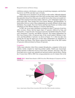
!
&F(K, L)/&L
&F(K, L)/&K
&H
&*
! Q " F(K, L) ! 0
&H
&K
! r " *
&F(K, L)
&K
! 0
&H
&L
! w " *
&F(K, L)
&L
! 0
H ! wL % rK % *[Q " F(K, L)]
wL % rK subject to F(K, L) ! Q
dK
dL
! "
MPL
MPK
&F(K, L)/&K ! MPK
&F(K, L)/&L ! MPL
dK
dL
! "
&F(K, L)/&L
&F(K, L)/&K](https://image.slidesharecdn.com/managerialeconomicsmichaelbaye2-230815092539-2513f09d/85/Managerial_economics_michael_baye-2-pdf-233-320.jpg)
![The Production Process and Costs 201
here), average cost is AC(Q) ! C(Q)/Q. The change in average cost due to a change in out-
put is simply the derivative of average cost with respect to output. Taking the derivative of
AC(Q) with respect to Q and using the quotient rule, we see that
since dC(Q)/dQ ! MC(Q). Thus, when MC(Q) ' AC(Q), average cost declines as output
increases. When MC(Q) ( AC(Q), average cost rises as output increases. Finally, when
MC(Q) ! AC(Q), average cost is at its minimum.
dAC(Q)
dQ
!
Q(dC/dQ) " C(Q)
Q2
!
1
Q
[MC(Q) " AC(Q)]](https://image.slidesharecdn.com/managerialeconomicsmichaelbaye2-230815092539-2513f09d/85/Managerial_economics_michael_baye-2-pdf-234-320.jpg)
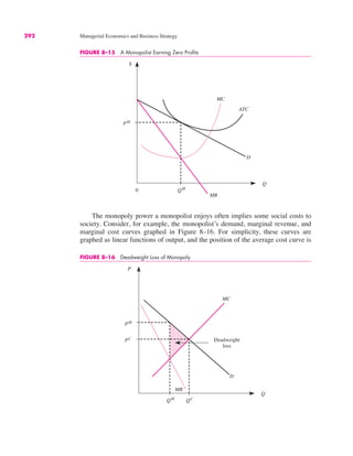
![270 Managerial Economics and Business Strategy
Demonstration Problem 8–1
The cost function for a firm is given by
If the firm sells output in a perfectly competitive market and other firms in the industry
sell output at a price of $20, what price should the manager of this firm put on the product?
What level of output should be produced to maximize profits? How much profit will be
earned?
(Hint: Recall that for a cubic cost function
the marginal cost function is
Since a ! 0, b ! 1, and c ! 0 for the cost function in this problem, we see that the marginal
cost function for the firm is MC(Q) ! 2Q.)
MC(Q) ! a % 2bQ % 3cQ2
C(Q) ! f % aQ % bQ2 % cQ3
C(Q) ! 5 % Q2
Principle Competitive Output Rule
To maximize profits, a perfectly competitive firm produces the output at which price
equals marginal cost in the range over which marginal cost is increasing:
P ! MC(Q)
the height [Pe
$ ATC(Q*)]. Recall that ATC(Q*) ! C(Q*)/Q*; that is, average total
cost is total cost divided by output. The area of the shaded rectangle is
which is the definition of profits. Intuitively, [Pe
$ ATC(Q*
)] represents the profits
per unit produced. When this is multiplied by the profit-maximizing level of output
(Q*), the result is the amount of total profits earned by the firm.
Q*
!Pe $
C(Q*)
Q* "! PeQ* $ C(Q*)
A Calculus
Alternative
The profits of a perfectly competitive firm are
The first-order condition for maximizing profits requires that the marginal profits be zero:
Thus, we obtain the profit-maximizing rule for a firm in perfect competition:
or
P ! MC
P !
dC
dQ
d#
dQ
! P $
dC(Q)
dQ
! 0
# ! PQ $ C(Q)](https://image.slidesharecdn.com/managerialeconomicsmichaelbaye2-230815092539-2513f09d/85/Managerial_economics_michael_baye-2-pdf-303-320.jpg)
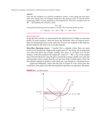
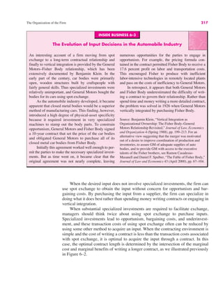
![0
$
Q*
MC
ATC (Q*)
ATC
AVC
Df
= Pe
= MR
Loss if
produce
Pe
AVC (Q*)
Loss if
shut down
Fixed
cost
Firm’s output
FIGURE 8–5 The Shut-Down Case
272 Managerial Economics and Business Strategy
the firm would not earn zero economic profits if it shut down but would instead
realize a loss equal to these fixed costs. Since the price in Figure 8–4 exceeds the
average variable cost of producing Q* units of output, the firm earns revenues on
each unit sold that are more than enough to cover the variable cost of producing
each unit. By producing Q* units of output, the firm is able to put an amount of
money into its cash drawer that exceeds the variable costs of producing these units
and thus contributes toward the firm’s payment of fixed costs. In short, while the
firm in Figure 8–4 suffers a short-run loss by operating, this loss is less than the loss
that would result if the firm completely shut down its operation.
The Decision to Shut Down. Now suppose the market price is so low that it lies
below the average variable cost, as in Figure 8–5. If the firm produced Q*, where
Pe
! MC in the range of increasing marginal cost, it would incur a loss equal to the
sum of the two shaded rectangles in Figure 8–5. In other words, for each unit sold,
the firm would lose
When this per-unit loss is multiplied by Q*, negative profits result that corre-
spond to the sum of the two shaded rectangles in Figure 8–5.
Now suppose that instead of producing Q* units of output this firm decided to
shut down its operation. In this instance, its losses would equal its fixed costs; that
is, those costs that must be paid even if no output is produced. Geometrically, fixed
costs are represented by the top rectangle in Figure 8–5, since the area of this rec-
tangle is
[ATC(Q*) $ AVC(Q*)]Q*
ATC(Q*) $ Pe](https://image.slidesharecdn.com/managerialeconomicsmichaelbaye2-230815092539-2513f09d/85/Managerial_economics_michael_baye-2-pdf-305-320.jpg)
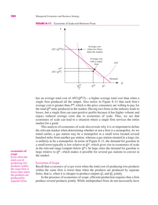
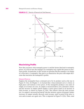
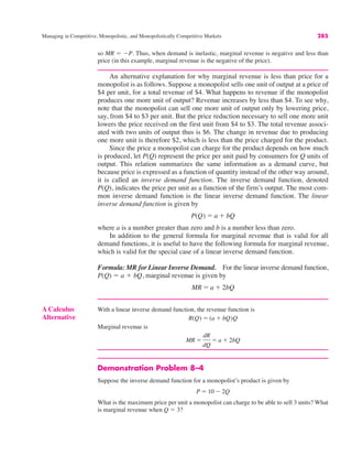
![Managing in Competitive, Monopolistic, and Monopolistically Competitive Markets 283
revenue is maximized at an output of Q0
in Figure 8–12(b). This corresponds to
the price of P0
in Figure 8–12(a), where demand is unitary elastic.
The line labeled MR in Figure 8–12(a) is the marginal revenue schedule for the
monopolist. Recall that marginal revenue is the change in total revenue attributable
to the last unit of output; geometrically, it is the slope of the total revenue curve.
As Figure 8–12(a) shows, the marginal revenue schedule for a monopolist lies
below the demand curve; in fact, for a linear demand curve, the marginal revenue
schedule lies exactly halfway between the demand curve and the vertical axis. This
means that for a monopolist, marginal revenue is less than the price charged for the
good.
There are two ways to understand why the marginal revenue schedule lies
below the monopolist’s demand curve. Consider first a geometric explanation.
Marginal revenue is the slope of the total revenue curve [R(Q)] in Figure 8–12(b).
As output increases from zero to Q0
, the slope of the total revenue curve decreases
until it becomes zero at Q0
. Over this range, marginal revenue decreases until it
reaches zero when output is Q0
. As output expands beyond Q0
, the slope of the
total revenue curve becomes negative and gets increasingly negative as output
continues to expand. This means that marginal revenue is negative for outputs in
excess of Q0
.
Formula: Monopolist’s Marginal Revenue. The marginal revenue of a monopolist is
given by the formula
where E is the elasticity of demand for the monopolist’s product and P is the price charged
for the product.
MR ! P!
1 % E
E "
INSIDE BUSINESS 8–2
Patent, Trademark, and Copyright Protection
The United States grants inventors three types of
patent protection: utility, design, and plant patents.
A “utility patent” protects the way an invention is
used and works, while a “design patent” protects
the way an invention looks. A “plant patent” pro-
tects an inventor who has discovered and asexually
reproduced a distinct and new variety of plant
(excluding tuber propagated plants or plants found
in uncultivated states). Utility and plant patents
provide 20 years of protection, while design patents
last 14 years.
Trademarks are different from patents in that they
protect words, names, symbols, or images that are used
in connection with goods or services. Similarly, a copy-
right protects a creator’s form of expression (including
literary, dramatic, musical, and artistic works). Patents
and trademarks are administered through the U.S.
Patent and Trademark Office, while the U.S. Copyright
Office handles copyrights.
Sources: United States Patent and Trademark Office; United
States Copyright Office.](https://image.slidesharecdn.com/managerialeconomicsmichaelbaye2-230815092539-2513f09d/85/Managerial_economics_michael_baye-2-pdf-316-320.jpg)
![286 Managerial Economics and Business Strategy
Answer:
First, we set Q ! 3 in the inverse demand function (here a ! 10 and b ! $2) to get
Thus, the maximum price per unit the monopolist can charge to be able to sell 3 units is $4.
To find marginal revenue when Q ! 3, we set Q ! 3 in the marginal revenue formula for
linear inverse demand to get
The Output Decision
Revenues are one determinant of profits; costs are the other. Since the revenue a
monopolist receives from selling Q units is R(Q) ! Q[P(Q)], the profits of a
monopolist with a cost function of C(Q) are
Typical revenue and cost functions are graphed in Figure 8–13(a). The vertical
distance between the revenue and cost functions in panel (a) reflects the profits to
the monopolist of alternative levels of output. Output levels below point A and
above point B imply losses, since the cost curve lies above the revenue curve. For
output levels between points A and B, the revenue function lies above the cost func-
tion, and profits are positive for those output levels.
Figure 8–13(b) depicts the profit function, which is the difference between R
and C in panel (a). As Figure 8–13(a) shows, profits are greatest at an output of QM
,
where the vertical distance between the revenue and cost functions is the greatest.
This corresponds to the maximum profit point in panel (b). A very important prop-
erty of the profit-maximizing level of output (QM
) is that the slope of the revenue
function in panel (a) equals the slope of the cost function. In economic terms, mar-
ginal revenue equals marginal cost at an output of QM
.
# ! R(Q) $ C(Q)
MR ! 10 $ [(2)(2)(3)] ! $2
P ! 10 $ 2(3) ! 4
Principle Monopoly Output Rule
A profit-maximizing monopolist should produce the output, QM
, such that marginal rev-
enue equals marginal cost:
MR(QM) ! MC(QM)
A Calculus
Alternative
The profits for a monopolist are
where R(Q) is total revenue. To maximize profits, marginal profits must be zero:
or
MR ! MC
d#
dQ
!
dR(Q)
dQ
$
dC(Q)
dQ
! 0
# ! R(Q) $ C(Q)](https://image.slidesharecdn.com/managerialeconomicsmichaelbaye2-230815092539-2513f09d/85/Managerial_economics_michael_baye-2-pdf-319-320.jpg)
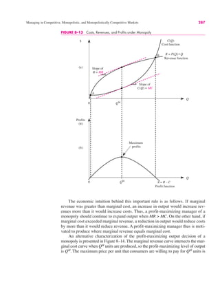
![$
Q
ATC
PM
ATC (QM
)
QM
Profits = [PM
– ATC (QM
)] " QM
Profits
MC
D
MR
288 Managerial Economics and Business Strategy
PM
, so the profit-maximizing price is PM
. Monopoly profits are given by the shaded
rectangle in the figure, which is the base (QM
) times the height [PM
$ ATC(QM
)].
FIGURE 8–14 Profit Maximization under Monopoly
Principle Monopoly Pricing Rule
Given the level of output, QM
, that maximizes profits, the monopoly price is the price on
the demand curve corresponding to the QM
units produced:
PM ! P(QM)
Demonstration Problem 8–5
Suppose the inverse demand function for a monopolist’s product is given by
and the cost function is given by
Determine the profit-maximizing price and quantity and the maximum profits.
Answer:
Using the marginal revenue formula for linear inverse demand and the formula for marginal
cost, we see that
MR ! 100 $ (2)(2)(Q) ! 100 $ 4Q
MC ! 2
C(Q) ! 10 % 2Q
P ! 100 $ 2Q](https://image.slidesharecdn.com/managerialeconomicsmichaelbaye2-230815092539-2513f09d/85/Managerial_economics_michael_baye-2-pdf-321-320.jpg)
![Managing in Competitive, Monopolistic, and Monopolistically Competitive Markets 289
Next, we set MR ! MC to find the profit-maximizing level of output:
or
Solving for Q yields the profit-maximizing output of QM
! 24.5 units. We find the profit-
maximizing price by setting Q ! QM
in the inverse demand function:
Thus, the profit-maximizing price is $51 per unit. Finally, profits are given by the difference
between revenues and costs:
The Absence of a Supply Curve
Recall that a supply curve determines how much will be produced at a given
price. Since perfectly competitive firms determine how much output to pro-
duce based on price (P ! MC), supply curves exist in perfectly competitive
markets. In contrast, a monopolist determines how much to produce based on
marginal revenue, which is less than price (P > MR ! MC). As a consequence,
there is no supply curve in markets served by firms with market power—such
as a monopolist.
Multiplant Decisions
Up until this point, we have assumed that the monopolist produces output at a sin-
gle location. In many instances, however, a monopolist has different plants at dif-
ferent locations. An important issue for the manager of such a multiplant monopoly
is the determination of how much output to produce at each plant.
Suppose the monopolist produces output at two plants. The cost of producing
Q1 units at plant 1 is C1(Q1), and the cost of producing Q2 units at plant 2 is C2(Q2).
Further, suppose the products produced at the two plants are identical, so the price
per unit consumers are willing to pay for the total output produced at the two plants
is P(Q), where
Profit maximization implies that the two-plant monopolist should produce output in
each plant such that the marginal cost of producing in each plant equals the mar-
ginal revenue of total output.
Q ! Q1 % Q2
! $1,190.50
! (51)(24.5) $ [10 % 2(24.5)]
# ! PMQM $ C(QM)
P ! 100 $ 2(24.5) ! 51
4Q ! 98
100 $ 4Q ! 2](https://image.slidesharecdn.com/managerialeconomicsmichaelbaye2-230815092539-2513f09d/85/Managerial_economics_michael_baye-2-pdf-322-320.jpg)
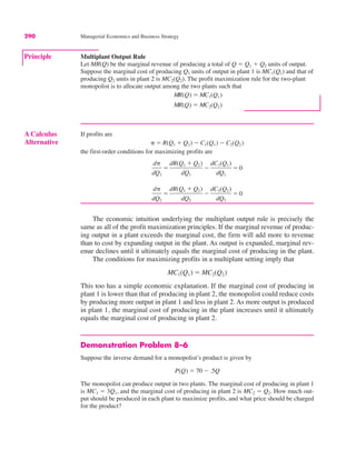
![$
Q
ATC
P*
Q*
MC
D
MR
0
Profits = [P* – ATC (Q*)] " Q*
ATC (Q*)
294 Managerial Economics and Business Strategy
product that differs slightly from other firms’ products. The products are close, but
not perfect, substitutes. For example, other things being equal, some consumers pre-
fer McDonald’s hamburgers, whereas others prefer to eat at Wendy’s, Burger King,
or one of the many other restaurants that serve hamburgers. As the price of a
McDonald’s hamburger increases, some consumers will substitute toward hamburgers
produced by another firm. But some consumers may continue to eat at McDonald’s
even if the price is higher than at other restaurants. The fact that the products are not
perfect substitutes in a monopolistically competitive industry thus implies that each
firm faces a downward-sloping demand curve for its product. To sell more of its
product, the firm must lower the price. In this sense, the demand curve facing a
monopolistically competitive firm looks more like the demand for a monopolist’s
product than like the demand for a competitive firm’s product.
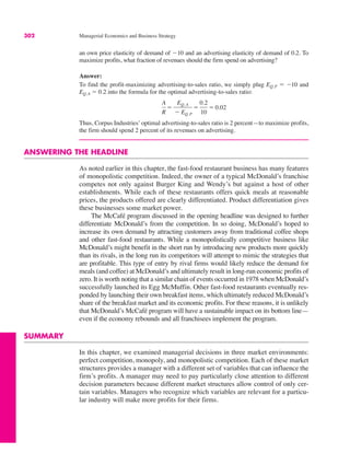
There are two important differences between a monopolistically competitive
market and a market serviced by a monopolist. First, while a monopolistically com-
petitive firm faces a downward-sloping demand for its product, there are other
firms in the industry that sell similar products. Second, in a monopolistically com-
petitive industry, there are no barriers to entry. As we will see later, this implies that
firms will enter the market if existing firms earn positive economic profits.
Profit Maximization
The determination of the profit-maximizing price and output under monopolistic
competition is precisely the same as for a firm operating under monopoly. To see
this, consider the demand curve for a monopolistically competitive firm presented in
Figure 8–17. Since the demand curve slopes downward, the marginal revenue curve
lies below it, just as under monopoly. To maximize profits, the monopolistically
FIGURE 8–17 Profit Maximization under Monopolistic Competition](https://image.slidesharecdn.com/managerialeconomicsmichaelbaye2-230815092539-2513f09d/85/Managerial_economics_michael_baye-2-pdf-327-320.jpg)
![296 Managerial Economics and Business Strategy
Next, we set MR ! MC to find the profit-maximizing level of output:
or
Solving for Q yields the profit-maximizing output of Q* ! 24.5 units. The profit-maximizing
price is found by setting Q ! Q* in the inverse demand function:
Thus, the profit-maximizing price is $51 per unit. Finally, profits are given by the difference
between revenues and costs:
Long-Run Equilibrium
Because there is free entry into monopolistically competitive markets, if firms
earn short-run profits in a monopolistically competitive industry, additional firms
will enter the industry in the long run to capture some of those profits. Similarly,
if existing firms incur losses, in the long run some firms will exit the industry.
! $1,195.50
! (51)(24.5) $ [5 % 2(24.5)]
# ! P*Q* $ C(Q*)
P* ! 100 $ 2 " 24.5 ! 51
4Q ! 98
100 $ 4Q ! 2
INSIDE BUSINESS 8–3
Product Differentiation, Cannibalization, and Colgate’s Smile
In 1896, Colgate dental cream was introduced in tubes
similar to those we use now. Today, the Colgate-
Palmolive Company’s brand of toothpaste is the best-
selling toothpaste in the world (ahead of the Crest
brand marketed by Procter & Gamble, which was
introduced in 1955).
While Colgate and Crest enjoy the lion’s share of
the toothpaste market, if you view the oral care shelf
at your local drugstore or supermarket you will find
over a hundred different varieties of toothpaste. Col-
gate alone sells over 40 different varieties that are
marketed under names ranging from Shrek Bubble
Fruit to Colgate Total Advanced Whitening.
Why would a dominant company like Colgate
choose to sell so many different varieties of tooth-
paste—varieties that compete against each other for
consumers’ dollars?
The high level of product differentiation in the
toothpaste market stems from firms introducing new
varieties in an attempt to boost their economic profits.
In environments where makers of other brands (such
as Crest) can easily enter profitable segments of the
market, a profitable strategy is to attempt to quickly
cover that segment (introducing Shrek Bubble Fruit
toothpaste, for instance) in order to earn short-run
profits until other firms enter to steal a share of that
segment. While introducing new varieties may canni-
balize sales of your existing products, cannibalizing
your own sales is better than having them stolen by a
hungry competitor.
Sources: Corporate Web sites of the Colgate-Palmolive
Company and Procter & Gamble and Hoover’s Online.](https://image.slidesharecdn.com/managerialeconomicsmichaelbaye2-230815092539-2513f09d/85/Managerial_economics_michael_baye-2-pdf-329-320.jpg)
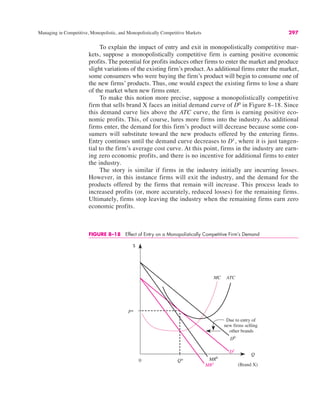
![Managing in Competitive, Monopolistic, and Monopolistically Competitive Markets 301
Two aspects of this formula are worth noting. First, the more elastic the demand
for a firm’s product, the lower the optimal advertising-to-sales ratio. In the extreme
case where EQ,P ! $( (perfect competition), the formula indicates that the optimal
advertising-to-sales ratio is zero. Second, the greater the advertising elasticity, the
greater the optimal advertising-to-sales ratio. Firms that have market power (such as
monopolists and monopolistically competitive firms) face a demand curve that is not
perfectly elastic. As a consequence, these firms will generally find it optimal to
engage in some degree of advertising. Exactly how much such firms should spend on
advertising, however, depends on the quantitative impact of advertising on demand.
The more sensitive demand is to advertising (that is, the greater the advertising elas-
ticity), the greater the number of additional units sold because of a given increase in
advertising expenditures, and thus the greater the optimal advertising-to-sales ratio.
Demonstration Problem 8–8
Corpus Industries produces a product at constant marginal cost that it sells in a monopolistically
competitive market. In an attempt to bolster profits, the manager hired an economist to estimate
the demand for its product. She found that the demand for the firm’s product is log-linear, with
A Calculus
Alternative
A firm’s profits are revenues minus production costs and advertising expenditures. If we let
A represent advertising expenditures, Q ! Q(P, A) denote the demand for the firm’s prod-
uct, and C(Q) denote production costs, firm profit is a function of P and A:
The first-order conditions for maximizing profits require
(8–1)
and
(8–2)
Noting that ∂C/∂Q ! MC and EQ,P ! (∂Q/∂P)(P/Q), we may write Equation (8–1) as
(8–3)
Similarly, using the fact that EQ,A ! (∂Q/∂A)(A/Q), Equation (8–2) implies
(8–4)
Substituting Equation (8–3) into Equation (8–4) yields the above formula.
A
R
! ¢
P $ MC
P
≤EQ,A
P $ MC
P
!
$1
EQ,P
)#
)A
!
)Q
)A
P $
)C
)Q
)Q
)A
$ 1 ! 0
)#
)P
!
)Q
)P
P % Q $
)C
)Q
)Q
)P
! 0
#(P, A) ! Q(P, A)P $ C[Q(P, A)] $ A
where EQ,P represents the own-price elasticity of demand for the firm’s product,
EQ,A is the advertising elasticity of demand for the firm’s product, A represents the
firm’s expenditures on advertising, and R ! PQ denotes the dollar value of the
firm’s sales (that is, the firm’s revenues).](https://image.slidesharecdn.com/managerialeconomicsmichaelbaye2-230815092539-2513f09d/85/Managerial_economics_michael_baye-2-pdf-334-320.jpg)
![A Calculus
Alternative
Firm 1’s revenues are
Thus,
A similar analysis yields the marginal revenue for firm 2.
MR1(Q1, Q2) "
%R1
%Q1
" a # bQ2 # 2bQ1
R1 " PQ1 " [a # b(Q1 $ Q2)]Q1
Basic Oligopoly Models 321
where a and b are positive constants, then the marginal revenues of firms 1 and 2 are
MR2(Q1, Q2) " a # bQ1 # 2bQ2
MR1(Q1, Q2) " a # bQ2 # 2bQ1
Notice that the marginal revenue for each Cournot oligopolist depends not only
on the firm’s own output but also on the other firm’s output. In particular, when
firm 2 increases its output, firm 1’s marginal revenue falls. This is because the
increase in output by firm 2 lowers the market price, resulting in lower marginal
revenue for firm 1.
Since each firm’s marginal revenue depends on its own output and that of the
rival, the output where a firm’s marginal revenue equals marginal cost depends on the
other firm’s output level. If we equate firm 1’s marginal revenue with its marginal
cost and then solve for firm 1’s output as a function of firm 2’s output, we obtain an
algebraic expression for firm 1’s reaction function. Similarly, by equating firm 2’s
marginal revenue with marginal cost and performing some algebra, we obtain firm
2’s reaction function. The results of these computations are summarized below.
Formula: Reaction Functions for Cournot Duopoly. For the linear (inverse)
demand function
and cost functions,
the reaction functions are
Q2 " r2(Q1) "
a # c2
2b
#
1
2
Q1
Q1 " r1(Q2) "
a # c1
2b
#
1
2
˛Q2
C2(Q2) " c2Q2
C1(Q1) " c1Q1
P " a # b(Q1 $ Q2)](https://image.slidesharecdn.com/managerialeconomicsmichaelbaye2-230815092539-2513f09d/85/Managerial_economics_michael_baye-2-pdf-354-320.jpg)
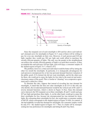
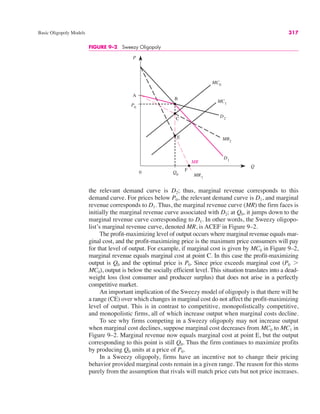
![336 Managerial Economics and Business Strategy
When would this “price war” end? When each firm charged a price that
equaled marginal cost: P1 " P2 " MC. Given the price of the other firm, neither
firm would choose to lower its price, for then its price would be below marginal
cost and it would make a loss. Also, no firm would want to raise its price, for then
it would sell nothing. In short, Bertrand oligopoly and homogeneous products lead
to a situation where each firm charges marginal cost and economic profits are zero.
Since P " MC, homogeneous product Bertrand oligopoly results in a socially efficient
level of output. Indeed, total market output corresponds to that in a perfectly com-
petitive industry, and there is no deadweight loss.
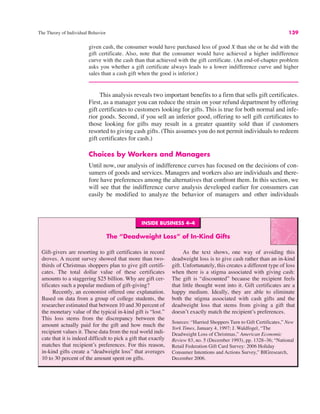
Chapters 10 and 11 provide strategies that managers can use to mitigate the
“Bertrand trap”—the cut-throat competition that ensues in homogeneous-product
Bertrand oligopoly. As we will see, the key is to either raise switching costs or elim-
inate the perception that the firms’ products are identical. The product differentia-
tion induced by these strategies permits firms to price above marginal cost without
losing customers to rivals. The appendix to this chapter illustrates that, under dif-
ferentiated-product price competition, reaction functions are upward sloping and
equilibrium occurs at a point where prices exceed marginal cost. This explains, in
part, why firms such as Kellogg’s and General Mills spend millions of dollars on
advertisements designed to persuade consumers that their competing brands of corn
flakes are not identical. If consumers did not view the brands as differentiated prod-
ucts, these two makers of breakfast cereal would have to price at marginal cost.
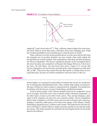
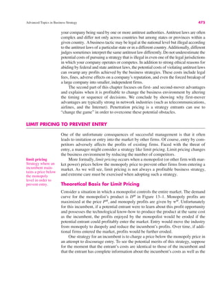
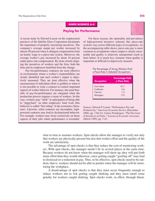
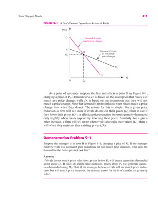
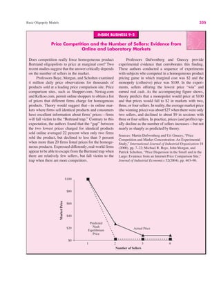
COMPARING OLIGOPOLY MODELS
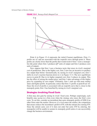
To see further how each form of oligopoly affects firms, it is useful to compare the
models covered in this chapter in terms of individual firm outputs, prices in the
market, and profits per firm. To accomplish this, we will use the same market
demand and cost conditions for each firm when examining results for each model.
The inverse market demand function we will use is
The cost function of each firm is identical and given by
so the marginal cost of each firm is 4. We will now see how outputs, prices, and prof-
its vary according to the type of oligopolistic interdependence that exists in the market.
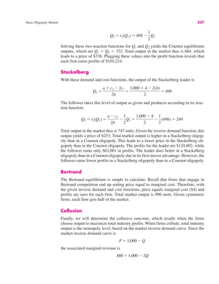
Cournot
We will first examine Cournot equilibrium. The profit function for the individual
Cournot firm given the preceding inverse demand and cost functions is
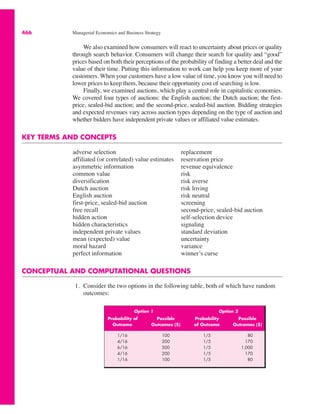
The reaction functions of the Cournot oligopolists are
Q1 " r1(Q2) " 498 #
1
2
Q2
&i " [1,000 # (Q1 $ Q2)]Qi # 4Qi
Ci(Qi) " 4Qi
P " 1,000 # (Q1 $ Q2)](https://image.slidesharecdn.com/managerialeconomicsmichaelbaye2-230815092539-2513f09d/85/Managerial_economics_michael_baye-2-pdf-369-320.jpg)