Downloaded 87 times


![+
Productivity Measures:Average
Product of an Input
Average Product of an Input: measure of
output produced per unit of input.
Average Product of Labor: APL = Q/L.
Measures the output of an “average” worker.
Example: Q = F(K,L) = K.5 L.5
If the inputs are K = 16 and L = 16, then the average product
of labor is APL = [(16) 0.5(16)0.5]/16 = 1.
Average Product of Capital:APK = Q/K.
Measures the output of an “average” unit of capital.
Example: Q = F(K,L) = K.5 L.5
If the inputs are K = 16 and L = 16, then the average product
of capital is APK = [(16)0.5(16)0.5]/16 = 1.
5-10
1](https://image.slidesharecdn.com/bayeall1-160112073144/75/Managerial-Economis-101-2048.jpg)


![Variable Cost
$
Q
ATC
AVC
MC
AVC
Variable Cost
Q0
Q0AVC
= Q0[VC(Q0)/ Q0]
= VC(Q0)
Minimum ofAVC
5-11
9](https://image.slidesharecdn.com/bayeall1-160112073144/75/Managerial-Economis-119-2048.jpg)
![$
Q
ATC
AVC
MC
ATC
Total Cost
Q0
= Q0[C(Q0)/ Q0]
= C(Q0)
Total Cost
Q0ATC
Minimum ofATC
5-12
0](https://image.slidesharecdn.com/bayeall1-160112073144/75/Managerial-Economis-120-2048.jpg)


![+ A Simple Markup Rule
Suppose the elasticity of demand for the firm’s product is
EF.
Since MR = P[1 + EF]/ EF.
Setting MR = M C and simplifying yields this simple pricing
formula:
P = [EF/(1+ EF)] MC.
The optimal price is a simple markup over relevant costs!
More elastic the demand, lower markup.
Less elastic the demand, higher markup.
11-2
12](https://image.slidesharecdn.com/bayeall1-160112073144/75/Managerial-Economis-212-2048.jpg)
![+ An Example
Elasticity of demand for Kodak film is -2.
P = [EF/(1+ EF)] M C
P = [-2/(1 - 2)] M C
P = 2 M C
Price is twice marginal cost.
Fifty percent of Kodak’s price is margin above manufacturing
costs.
11-2
13](https://image.slidesharecdn.com/bayeall1-160112073144/75/Managerial-Economis-213-2048.jpg)
![+Markup Rule for Cournot Oligopoly
Homogeneous product Cournotoligopoly.
N = total number of firms in the industry.
Market elasticity of demand EM .
Elasticity of individual firm’s demand is given
by EF = N x EM.
Since P = [EF/(1+ EF)] MC,
Then, P = [NEM/(1+ NEM)] MC.
The greater the number of firms, the lower the
profit-maximizing markup factor.
11-2
14](https://image.slidesharecdn.com/bayeall1-160112073144/75/Managerial-Economis-214-2048.jpg)
![+ An Example
Homogeneous product Cournot industry, 3
firms.
M C = $10.
Elasticity of market demand = - ½.
Determine the profit-maximizingprice?
EF = N EM = 3 (-1/2) = -1.5.
P = [EF/(1+ EF)] MC.
P = [-1.5/(1- 1.5] $10.
P = 3 $10 = $30.
11-2
15](https://image.slidesharecdn.com/bayeall1-160112073144/75/Managerial-Economis-215-2048.jpg)


![+ Implementing Third-DegreePrice
Discrimination
Suppose the total demand for a product is
comprised of two groups with different
elasticities, E1< E2.
Notice that group 1 is more price sensitive than
group 2.
Profit-maximizing prices?
P1 = [E1/(1+ E1)] M C
P2 = [E2/(1+ E2)] M C
11-22
2](https://image.slidesharecdn.com/bayeall1-160112073144/75/Managerial-Economis-222-2048.jpg)
![+ An Example
Suppose the elasticity of demand for Kodak
film in the US is EU = -1.5,and the elasticity of
demand in Japan is EJ = -2.5.
Marginal cost of manufacturing film is $3.
PU = [EU/(1+ EU)] M C = [-1.5/(1 - 1.5)] $3 =
$9
PJ = [EJ/(1+ EJ)] M C = [-2.5/(1 - 2.5)] $3 =
$5
Kodak’s optimal third-degree pricing
strategy is to charge a higher price in the US,
where demand is less elastic.
11-22
3](https://image.slidesharecdn.com/bayeall1-160112073144/75/Managerial-Economis-223-2048.jpg)


![+ Costs andProfits with Block
Pricing
Price
Quantity
D
10
8
6
4
2
1 2 3 4 5
MC =AC
Profits* = [.5(8)(4) + (2)(4)] – (2)(4)
= $16
Costs = (2)(4) = $8
* Assuming no fixedcosts
11-23
0](https://image.slidesharecdn.com/bayeall1-160112073144/75/Managerial-Economis-230-2048.jpg)


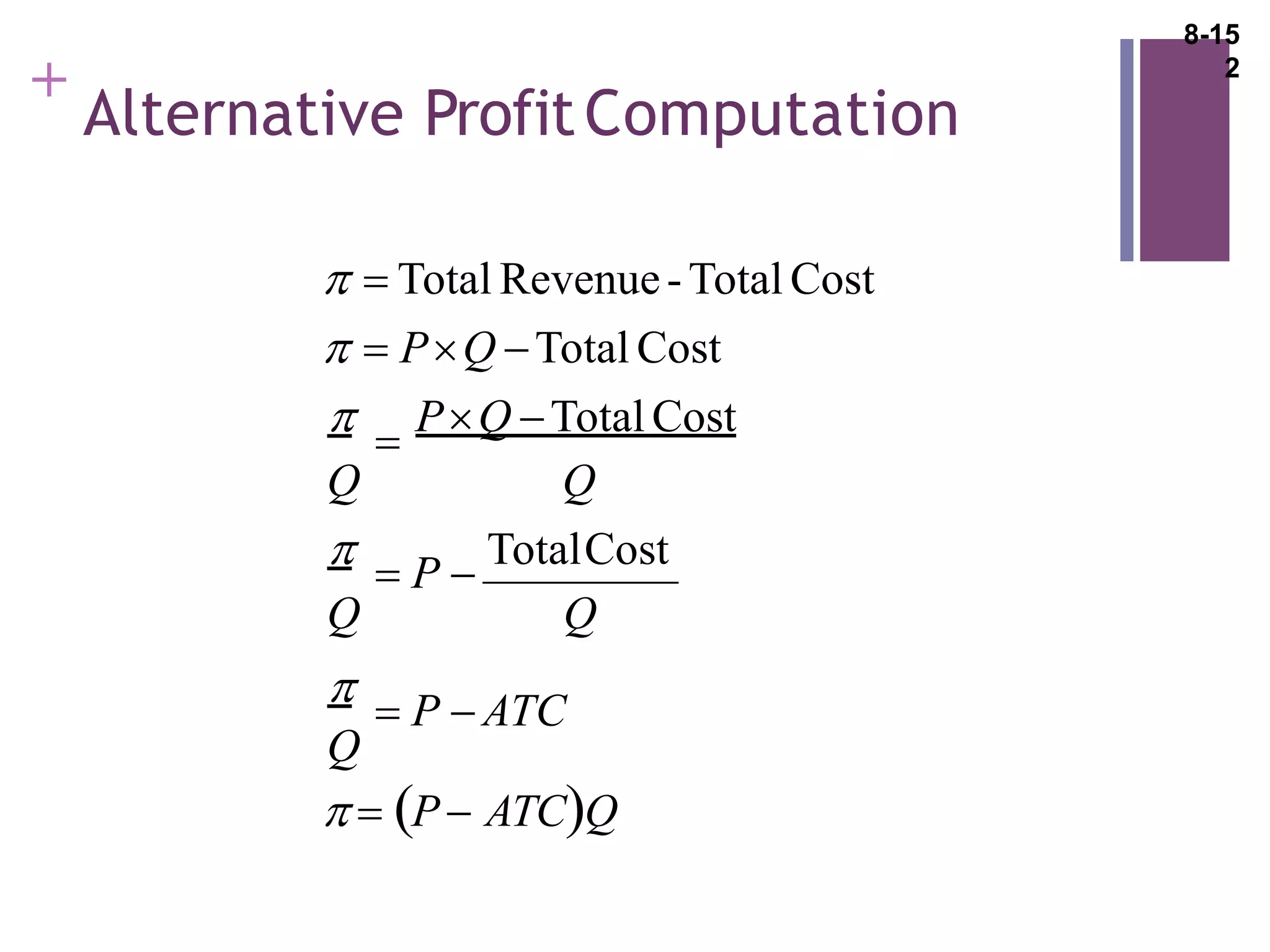
The document discusses key concepts in managerial economics including: - Managerial economics is the study of how managers direct scarce resources to efficiently achieve goals. - Economic and accounting profits are defined. Economic profits consider opportunity costs while accounting profits do not. - Profits signal where resources are most valued by society. Resources will flow to industries with highest profits. - Marginal analysis and the marginal principle of maximizing benefits when marginal benefits equal marginal costs.


