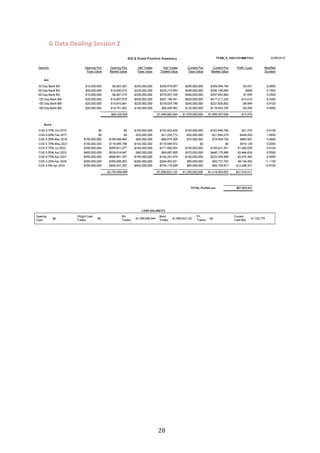
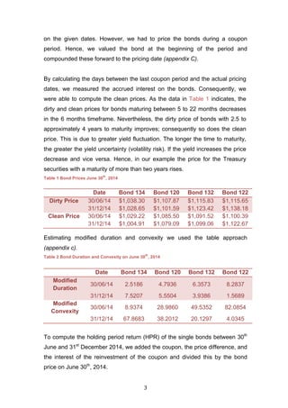
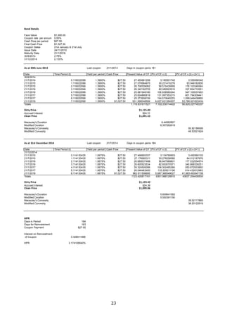
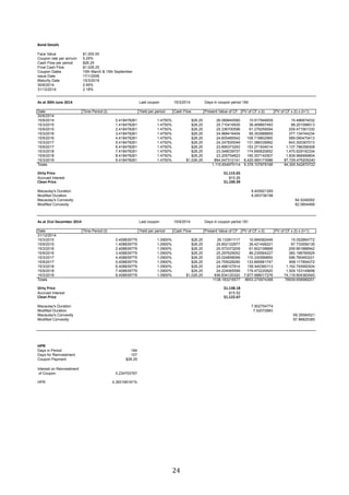
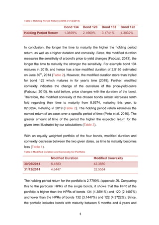
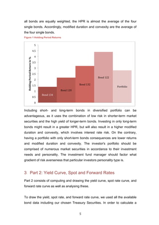
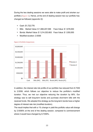
This document contains a report analyzing bond prices, yield curves, and a bond portfolio over time. It includes the following key points: - Bond prices from June 30th to December 31st decreased for short-term bonds but increased for mid-to-long term bonds, due to changes in yield. - Duration, a measure of price sensitivity, increased over time for longer-term bonds but decreased for shorter-term bonds. The portfolio's duration decreased from June to December as its average maturity shortened. 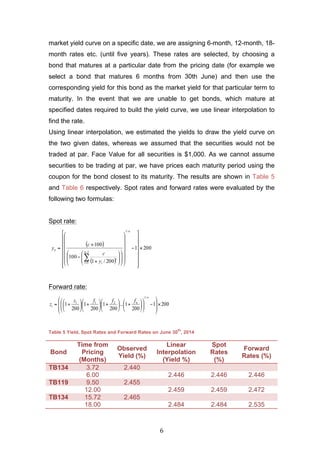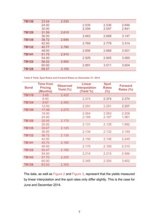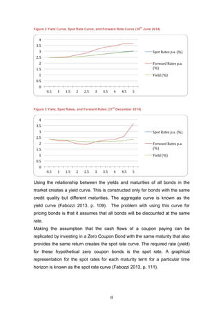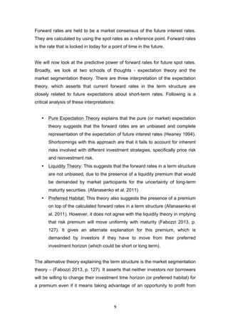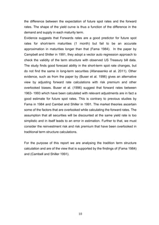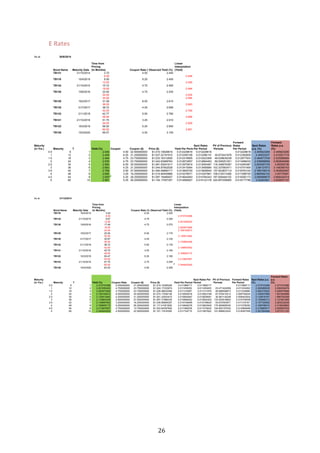- Yield curves, spot curves, and forward curves were constructed using bond data from the two dates. Forward rates were higher than spot rates, indicating an upward sloping yield curve and expected rising interest rates

1. Alexander
Vasiagin
-­‐
3526584
Devvrat
Patney
-­‐
3507599
Lea-­‐Marie
Lamm
-­‐
3481019
M a j o r
p r o j e c t
B A F I
1 0 6 5
M o n e y
M a r k e t s
a n d
F i x e d
I n c o m e
S e c u r i t i e s
Bond
Evaluation
and
Dealing
Simulation
Report

2. 1
Table of Contents
1 Introduction.................................................................................................2
2 Part 1: Prices, Modified Duration and Convexity ....................................2
3 Part 2: Yield Curve, Spot and Forward Rates ..........................................5
4 Part 3: Dealing Simulation Report ..........................................................11
Referencing ....................................................................................................15
Appendix.........................................................................................................16
Tables
Table 1 Bond Prices June 30th
, 2014.................................................................3
Table 2 Bond Duration and Convexity on June 30th
, 2014.................................3
Table 3 Holding Period Return (30/06-31/12/2014) ...........................................4
Table 4 Modified Duration and Convexity for Portfolio.......................................4
Table 5 Yield, Spot Rates and Forward Rates on June 30th
, 2014....................6
Table 6 Yield, Spot Rates and Forward Rates on December 31, 2014 .............7
Figures
Figure 1 Holding Period Returns........................................................................5
Figure 2 Yield Curve, Spot Rate Curve, and Forward Rate Curve (30th
June
2014)...........................................................................................................8
Figure 3 Yield, Spot Rates, and Forward Rates (31st
December 2014).............8
Figure 4 Comparison Forward Rates 30th June to Spot Rates 31st December
..................................................................................................................11
Figure 5 Yield Curve ........................................................................................12
Figure 6 Portfolio Comparison .........................................................................13

3. 2
1 Introduction
For fulfilling the required task of our major project we chose the following on-
the-run Australian Government Securities:
• 4.75% Treasury Bonds due to 21st
October 2015 (bond 134)
• 6.00% Treasury Bonds due to 15th
February 2017 (bond 120)
• 5.50% Treasury Bonds due to 21st
January 2018 (bond 132)
• 5.25% Treasury Bonds due to 15th
March 2019 (bond 122)
The data was extracted from the website of Reserve Bank of Australia, using
the ‘Indicative Mid Rates of Australian Government Securities - 2013 to
Current’ (appendix A). To gather more detailed information on the bonds, we
used the relevant term sheets (appendix B). All Treasury Bonds are long-term
securities paying regular coupons at the end of two 6-month compounding
periods per year. Moreover, the bonds pay the face value at maturity.
To examine the predictive ability of the yield, spot and forward rate curves, this
report will first define what these each curves represents, subsequently we will
analyse the various theories and schools of thought that attempt to explain
expectation theory and their underlying assumptions.
Part 3 of the report summarizes our experience with the two dealing simulation
sessions with respect to the current yield curve in the Australian stock market
and the set objective.
2 Part 1: Prices, Modified Duration and Convexity
Part 1 of the project includes calculations of dirty price, clean price, modified
duration and modified convexity on 30th
June 2014 and 31st
December 2014.
To calculate the dirty price we discounted the coupons in the required period to
evaluate the present value per period and summed these to compute the price

4. 3
on the given dates. However, we had to price the bonds during a coupon
period. Hence, we valued the bond at the beginning of the period and
compounded these forward to the pricing date (appendix C).
By calculating the days between the last coupon period and the actual pricing
dates, we measured the accrued interest on the bonds. Consequently, we
were able to compute the clean prices. As the data in Table 1 indicates, the
dirty and clean prices for bonds maturing between 5 to 22 months decreases
in the 6 months timeframe. Nevertheless, the dirty price of bonds with 2.5 to
approximately 4 years to maturity improves; consequently so does the clean
price. This is due to greater yield fluctuation. The longer the time to maturity,
the greater the yield uncertainty (volatility risk). If the yield increases the price
decrease and vice versa. Hence, in our example the price for the Treasury
securities with a maturity of more than two years rises.
Table 1 Bond Prices June 30
th
, 2014
Estimating modified duration and convexity we used the table approach
(appendix c).
Table 2 Bond Duration and Convexity on June 30
th
, 2014
To compute the holding period return (HPR) of the single bonds between 30th
June and 31st
December 2014, we added the coupon, the price difference, and
the interest of the reinvestment of the coupon and divided this by the bond
price on June 30th
, 2014.
Date Bond 134 Bond 120 Bond 132 Bond 122
Dirty Price 30/06/14 $1,038.30 $1,107.87 $1,115.83 $1,115.65
31/12/14 $1,028.65 $1,101.59 $1,123.42 $1,138.18
Clean Price 30/06/14 $1,029.22 $1,085.50 $1,091.52 $1,100.39
31/12/14 $1,004.91 $1,079.09 $1,099.06 $1,122.67
Date Bond 134 Bond 120 Bond 132 Bond 122
Modified
Duration
30/06/14 2.5186 4.7936 6.3573 8.2837
31/12/14 7.5207 5.5504 3.9386 1.5689
Modified
Convexity
30/06/14 8.9374 28.9860 49.5352 82.0854
31/12/14 67.8683 38.2012 20.1297 4.0345

5. 4
Table 3 Holding Period Return (30/06-31/12/2014)
Bond 134 Bond 120 Bond 132 Bond 122
Holding Period Return 1.3699% 2.1669% 3.1741% 4.3932%
In conclusion, the longer the time to maturity the higher the holding period
return, as well as a higher duration and convexity. Since, the modified duration
measures the sensitivity of a bond’s price to yield changes (Fabozzi, 2013), the
longer the time to maturity the stronger the sensitivity. For example bond 134
matures in 2015, and hence has a low modified duration of 2.5186 estimated
on June 30th
, 2014 (Table 2). However, the modified duration more than tripled
for bond 122 which matures in for year’s time (2019). Further, modified
convexity indicates the change of the curvature of the price-yield-curve
(Fabozzi, 2013). As said before, price changes with the duration of the bond.
Therefore, the modified convexity of the chosen bonds almost increases tenth
fold regarding their time to maturity from 8.9374, maturing this year, to
82.0854, maturing in 2019 (Table 2). The holding period return estimates the
earned return of an asset over a specific period of time (Pinto et al. 2010). The
greater amount of time of the period the higher the expected return for the
given time; illustrated by our calculations (Table 3).
With an equally weighted portfolio of the four bonds, modified duration and
convexity decrease between the two given dates, as time to maturity becomes
less (Table 4).
Table 4 Modified Duration and Convexity for Portfolio
Modified Duration Modified Convexity
30/06/2014 5.4883 42.3860
31/12/2014 4.6447 32.5584
The holding period return for the portfolio is 2.7799% (appendix D). Comparing
this to the particular HPRs of the single bonds, it shows that the HPR of the
portfolio is higher than the HPRs of bonds 134 (1.3591%) and 120 (2.1407%)
and lower than the HPRs of bonds 132 (3.1447%) and 122 (4.3722%). Since,
the portfolio includes bonds with maturity between 5 months and 4 years and

6. 5
all bonds are equally weighted, the HPR is almost the average of the four
single bonds. Accordingly, modified duration and convexity are the average of
the four single bonds.
Figure 1 Holding Period Returns
Including short- and long-term bonds in diversified portfolio can be
advantageous, as it uses the combination of low risk in shorter-term market
securities and the high yield of longer-term bonds. Investing in only long-term
bonds might result in a greater HPR, but will also result in a higher modified
duration and convexity, which involves interest rate risk. On the contrary,
having a portfolio with only short-term bonds consequences are lower returns
and modified duration and convexity. The investor's portfolio should be
comprised of numerous market securities in accordance to their investment
needs and personality. The investment fund manager should factor what
gradient of risk averseness that particular investors personality type is.
3 Part 2: Yield Curve, Spot and Forward Rates
Part 2 consists of computing and drawing the yield curve, spot rate curve, and
forward rate curve as well as analysing these.
To draw the yield, spot rate, and forward rate curve, we used all the available
bond data including our chosen Treasury Securities. In order to calculate a
Bond
134
Bond
120
Bond
132
Bond
122
Portfolio
0
0.5
1
1.5
2
2.5
3
3.5
4
4.5
5
Holding
Period
Return
in
%

7. 6
market yield curve on a specific date, we are assigning 6-month, 12-month, 18-
month rates etc. (until five years). These rates are selected, by choosing a
bond that matures at a particular date from the pricing date (for example we
select a bond that matures 6 months from 30th June) and then use the
corresponding yield for this bond as the market yield for that particular term to
maturity. In the event that we are unable to get bonds, which mature at
specified dates required to build the yield curve, we use linear interpolation to
find the rate.
Using linear interpolation, we estimated the yields to draw the yield curve on
the two given dates, whereas we assumed that the securities would not be
traded at par. Face Value for all securities is $1,000. As we cannot assume
securities to be trading at par, we have prices each maturity period using the
coupon for the bond closest to its maturity. The results are shown in Table 5
and Table 6 respectively. Spot rates and forward rates were evaluated by the
following two formulas:
Spot rate:
Forward rate:
Table 5 Yield, Spot Rates and Forward Rates on June 30
th
, 2014
Bond
Time from
Pricing
(Months)
Observed
Yield (%)
Linear
Interpolation
(Yield %)
Spot
Rates
(%)
Forward
Rates (%)
TB134 3.72 2.440
6.00 2.446 2.446 2.446
TB119 9.50 2.455
12.00 2.459 2.459 2.472
TB134 15.72 2.465
18.00 2.484 2.484 2.535
( )
( )
2001
200/1
100
100
/1
1
1
×
⎥
⎥
⎥
⎥
⎥
⎥
⎦
⎤
⎢
⎢
⎢
⎢
⎢
⎢
⎣
⎡
−
⎟
⎟
⎟
⎟
⎟
⎠
⎞
⎜
⎜
⎜
⎜
⎜
⎝
⎛
⎟
⎟
⎠
⎞
⎜
⎜
⎝
⎛
⎟
⎟
⎠
⎞
⎜
⎜
⎝
⎛
+
−
+
=
∑
−
=
n
n
t
t
t
n
y
c
c
y
2001
200
1...
200
1
200
1
200
1
/1
211
×
⎟
⎟
⎠
⎞
⎜
⎜
⎝
⎛
−⎟⎟
⎠
⎞
⎜⎜
⎝
⎛
⎟
⎠
⎞
⎜
⎝
⎛
+⎟
⎠
⎞
⎜
⎝
⎛
+⎟
⎠
⎞
⎜
⎝
⎛
+⎟
⎠
⎞
⎜
⎝
⎛
+=
n
n
t
fffz
z

8. 7
TB130 23.54 2.530
24.00 2.535 2.536 2.690
30.00 2.594 2.597 2.841
TB120 31.59 2.610
36.00 2.683 2.688 3.147
TB135 36.72 2.695
42.00 2.769 2.778 3.314
TB132 42.77 2.780
48.00 2.856 2.868 3.501
TB141 51.75 2.910
54.00 2.929 2.945 3.560
TB122 56.52 2.950
60.00 2.991 3.011 3.604
TB126 69.57 3.105
Table 6 Yield, Spot Rates and Forward Rates on December 31, 2014
Bond
Time from
Pricing
(Months)
Observed
Yield (%)
Linear
Interpolation
(Yield %)
Spot
Rates
(%)
Forward
Rates (%)
TB119 3.45 2.425
6.00 2.374 2.374 2.374
TB134 9.67 2.300
12.00 2.291 2.291 2.207
TB130 17.49 2.270
18.00 2.264 2.263 2.208
24.00 2.189 2.187 1.961
TB120 25.55 2.170
30.00 2.131 2.128 1.892
TB135 30.67 2.125
36.00 2.134 2.132 2.149
TB132 36.72 2.135
42.00 2.150 2.148 2.249
TB141 45.70 2.160
48.00 2.170 2.169 2.315
TB122 50.47 2.180
54.00 2.214 2.215 2.586
TB143 57.70 2.255
60.00 2.345 2.354 3.602
TB126 63.52 2.305
The data, as well as Figure 2 and Figure 3, represent that the yields measured
by linear interpolation and the spot rates only differ slightly. This is the case for
June and December 2014.

9. 8
Figure 2 Yield Curve, Spot Rate Curve, and Forward Rate Curve (30
th
June 2014)
Figure 3 Yield, Spot Rates, and Forward Rates (31
st
December 2014)
Using the relationship between the yields and maturities of all bonds in the
market creates a yield curve. This is constructed only for bonds with the same
credit quality but different maturities. The aggregate curve is known as the
yield curve (Fabozzi 2013, p. 109). The problem with using this curve for
pricing bonds is that it assumes that all bonds will be discounted at the same
rate.
Making the assumption that the cash flows of a coupon paying can be
replicated by investing in a Zero Coupon Bond with the same maturity that also
provides the same return creates the spot rate curve. The required rate (yield)
for these hypothetical zero coupon bonds is the spot rate. A graphical
representation for the spot rates for each maturity term for a particular time
horizon is known as the spot rate curve (Fabozzi 2013, p. 111).
0
0.5
1
1.5
2
2.5
3
3.5
4
0.5
1
1.5
2
2.5
3
3.5
4
4.5
5
Spot
Rates
p.a.
(%)
Forward
Rates
p.a.
(%)
Yield
(%)
0
0.5
1
1.5
2
2.5
3
3.5
4
0.5
1
1.5
2
2.5
3
3.5
4
4.5
5
Spot
Rates
p.a.
(%)
Forward
Rates
p.a.
(%)
Yield
(%)

10. 9
Forward rates are held to be a market consensus of the future interest rates.
They are calculated by using the spot rates as a reference point. Forward rates
is the rate that is locked in today for a point of time in the future.
We will now look at the predictive power of forward rates for future spot rates.
Broadly, we look at two schools of thoughts - expectation theory and the
market segmentation theory. There are three interpretation of the expectation
theory, which asserts that current forward rates in the term structure are
closely related to future expectations about short-term rates. Following is a
critical analysis of these interpretations:
• Pure Expectation Theory explains that the pure (or market) expectation
theory suggests that the forward rates are an unbiased and complete
representation of the expectation of future interest rates (Heaney 1994).
Shortcomings with this approach are that it fails to account for inherent
risks involved with different investment strategies, specifically price risk
and reinvestment risk.
• Liquidity Theory: This suggests that the forward rates in a term structure
are not unbiased, due to the presence of a liquidity premium that would
be demanded by market participants for the uncertainty of long-term
maturity securities. (Afanasenko et al. 2011)
• Preferred Habitat: This theory also suggests the presence of a premium
on top of the calculated forward rates in a term structure (Afanasenko et
al. 2011). However, it does not agree with the liquidity theory in implying
that risk premium will move uniformly with maturity (Fabozzi 2013, p.
127). It gives an alternate explanation for this premium, which is
demanded by investors if they have to move from their preferred
investment horizon (which could be short or long term).
The alternative theory explaining the term structure is the market segmentation
theory – (Fabozzi 2013, p. 127). It asserts that neither investors nor borrowers
will be willing to change their investment time horizon (or preferred habitat) for
a premium even if it means taking advantage of an opportunity to profit from

11. 10
the difference between the expectation of future spot rates and the forward
rates. The shape of the yield curve is thus a function of the difference in the
demand and supply in each maturity term.
Evidence suggests that Forwards rates are a good predictor for future spot
rates for short-term maturities (1 month) but fail to be an accurate
approximation in maturities longer than that (Fama 1984). In the paper by
Campbell and Shiller in 1991, they adopt a vector auto regression approach to
check the validity of the term structure with observed US Treasury bill data.
The study finds good forecast ability in the short-term spot rate changes, but
do not find the same in long-term securities (Afanasenko et al. 2011). Other
evidence, such as from the paper by (Buser et al. 1996) gives an alternative
view by adjusting forward rate calculations with risk premium and other
overlooked biases. Buser et al. (1996) suggest that forward rates between
1963- 1993 which have been calculated with relevant adjustments are in fact a
good estimate for future spot rates. This is contrary to previous studies by
Fama in 1984 and Cambel and Shiller in 1991. The market theories ascertain
some of the factors that are overlooked while calculating the forward rates. The
assumption that all securities will be discounted at the same yield rate is too
simplistic and in itself leads to an error in estimation. Further to that, we must
consider the reinvestment risk and risk premium that have been overlooked in
traditional term structure calculations.
For the purpose of this report we are analysing the tradition term structure
calculation and are of the view that is supported by the findings of (Fama 1984)
and (Cambell and Shiller 1991).

12. 11
Figure 4 Comparison Forward Rates 30th June to Spot Rates 31st December
Aligned with academic research referenced previously, we have found that the
forward rates are a good estimator for future spot rates in only the short term.
As evident from Figure 4, we can see that forward rates become a weak
estimator as maturity terms increase. Comparing the estimated forward rates
on 30th
of June to the spot rates on 31st
of December (appendix E), it actually
states that the forward rates do not match the calculated spot rates. Instead
the forward rates are much higher.
4 Part 3: Dealing Simulation Report
In part 3 we describe the current yield curve and our experience with the two
commenced dealing simulation sessions as well as our given objectives.
On 22nd
May 2015, the shape for the current yield curve in Australian
Commonwealth Government Securities was relatively flat until the 1-year
maturity period, following which the curve was upward sloping for the rest of
the 20-year time horizon (Figure
5).
0
0.5
1
1.5
2
2.5
3
3.5
4
1
2
3
4
5
6
7
8
9
10
Spot
/
Forward
Rates
Time
to
Maturity
Forward
Rates
p.a.
(%)
Spot
Rates
p.a.
(%)

13. 12
Figure
5
Yield
Curve
The expectation of the market for the 6- and 12-month period is evident from
the yield curve shown in Figure
5. It shows that the market yield expectation for
the 6- and 12-month maturity periods remains the same between the two
pricing dates (8 May and 22 May). The implications for fixed-interest fund
managers that the shape and level of the current yield curve in Australian
Commonwealth Government Securities would be that; they have to adjust the
bond price on current bonds in the market in accordance to the change in the
current yield and its relationship to the face value of the particular bond. The
main role of fixed-interest rate fund managers is to take advantage of potential
market inefficiencies and to give their customers higher than expected return
(abnormal returns) as the yield curve fluctuates.
At the commencement of the first dealing session our portfolio had the
following positions (appendix F):
• Cash: The portfolio had a zero cash balance
• Bills: market value: $99,317.95 face value: $100,000
• Bonds: market value: $2,765,720.041 face value: $ 2,400,000
• Modified duration: 8.7359

14. 13
During the two dealing sessions we were able to make profit and shorten our
portfolio (Figure
6). Hence, at the end of dealing session two our portfolio has
changed as followed (appendix G):
• Cash: $1,722,776
• Bills: Market Value: $ 1,666,207.096 Face Value: $ 1,676,000
• Bonds: Market Value: $ 1,214,353.663 Face Value: $ 1,050,000
• Modified duration: 2.9356
Figure
6
Portfolio
Comparisons
In addition, the interest rate risk profile of our portfolio has reduced from 8.7359
to 2.9356, which follows our objective to reduce the portfolio’s modified
duration. Thus, we met our objective reducing the duration by 66%. Our
strategy was to sell long-term bonds and purchase short-term bills with the
received funds. We adopted this strategy as the long-term bonds have a higher
degree of interest rate risk (modified duration).
The result implies that with a 1% change in yield the portfolio value will change
by 2.9356% at the end of the dealing session, compared to commencement
where it would have changed by 8.7359%.
$0
$500,000
$1,000,000
$1,500,000
$2,000,000
$2,500,000
$3,000,000
Cash
Bills
(MV)
Bills
(FV)
Bonds
(MV)
Bonds
(FC)
Session
1
Session
2

15. 14
In summary, we were able to grasp a better understanding of the roles of price
takers and makers from dealing sessions one and two. At the second dealing
session, we assigned one member to be a price taker and the other to be a
price maker to reduced confusion with the bid and ask prices which let to a
more smooth operation and more transactions. Further, we tried to achieve the
best possible outcome in terms of profit, whilst reaching our main objective of
reducing the modified duration of our portfolio.

16. 15
Referencing
Afanasenko, D, Gischer, H, & Reichling, P 2011, ‘The Predictive Power of
Forward Rates: A Re-examination for Germany’, Investment Management And
Financial Innovations, vol. 8, no. 1, pp. 125-139
Buser, SA, Karolyi, GA, & Sanders, AB, 1996, ‘Adjusted Forward Rates as
Predictors of Future Spot Rates’, Journal of Fixed Income, vol. 6, pp.29-42
Heaney, R 1994, ‘Predictive Power of the Term Structure in Australia in the
late 1980’s: a note’, Accounting & Finance, vol. 34, no. 1, pp. 37-46
Fabozzi, FJ 2013, ‘Bond Markets, Analysis, And Strategies’, Pearson, Boston,
Massachusetts
Fama, EF 1984, ‘The Information in the Term Structure’, Journal of Financial
Economics, vol. 13, no. 4, pp. 509-576
Pinto, J, Henry, E, Robinson, TR, & Stowe, JD, ‘Equity Asset Valuation’, John
Wiley & Sons, Hoboken, New Jersey

17. 16
Appendix
A
Bond
data

18. 17
B
Term
sheet
W ' ϭ
dĞƌŵ ^ŚĞĞƚ ĨŽƌ ϰ͘ϳϱй dƌĞĂƐƵƌLJ ŽŶĚƐ ĚƵĞ Ϯϭ KĐƚŽďĞƌ ϮϬϭϱ
dŚŝƐ dĞƌŵ ^ŚĞĞƚ ƌĞůĂƚĞƐ ƚŽ ƚŚĞ ƐĞƌŝĞƐ ŽĨ dƌĞĂƐƵƌLJ ŽŶĚƐ ƌĞĨĞƌƌĞĚ ƚŽ ĂďŽǀĞ͘ /ƚ ŝƐ ƐƵƉƉůĞŵĞŶƚĂƌLJ ƚŽ͕
ĂŶĚ ƐŚŽƵůĚ ďĞ ƌĞĂĚ͕ ĂƐ ĂƉƉƌŽƉƌŝĂƚĞ͕ ŝŶ ĐŽŶũƵŶĐƚŝŽŶ ǁŝƚŚ ĞŝƚŚĞƌ ƚŚĞ /ŶĨŽƌŵĂƚŝŽŶ DĞŵŽƌĂŶĚƵŵ ĨŽƌ
dƌĞĂƐƵƌLJ ŽŶĚƐ Žƌ ƚŚĞ /ŶǀĞƐƚŽƌ /ŶĨŽƌŵĂƚŝŽŶ ^ƚĂƚĞŵĞŶƚ ĨŽƌ džĐŚĂŶŐĞͲƚƌĂĚĞĚ dƌĞĂƐƵƌLJ ŽŶĚƐ͘
ĨŝŶĂŶĐŝĂů ĂĚǀŝƐĞƌ ƌĞĐŽŵŵĞŶĚŝŶŐ ƚŽ Ă ƌĞƚĂŝů ĐůŝĞŶƚ ƚŚĂƚ ƚŚĞLJ ŝŶǀĞƐƚ ŝŶ ƚŚŝƐ dƌĞĂƐƵƌLJ ŽŶĚ ǀŝĂ ĂŶ
džĐŚĂŶŐĞͲƚƌĂĚĞĚ dƌĞĂƐƵƌLJ ŽŶĚ ŵƵƐƚ ƉƌŽǀŝĚĞ Ă ĐŽƉLJ ŽĨ ƚŚŝƐ dĞƌŵ ^ŚĞĞƚ ĂŶĚ ƚŚĞ ĐƵƌƌĞŶƚ ǀĞƌƐŝŽŶ ŽĨ
ƚŚĞ /ŶǀĞƐƚŽƌ /ŶĨŽƌŵĂƚŝŽŶ ^ƚĂƚĞŵĞŶƚ ĨŽƌ džĐŚĂŶŐĞͲƚƌĂĚĞĚ dƌĞĂƐƵƌLJ ŽŶĚƐ ƚŽ ƚŚĞ ĐůŝĞŶƚ͘
/^^hZ ŽŵŵŽŶǁĞĂůƚŚ ŽĨ ƵƐƚƌĂůŝĂ
/E^dZhDEd dƌĞĂƐƵƌLJ ŽŶĚƐ
hZZEz ƵƐƚƌĂůŝĂŶ ĚŽůůĂƌƐ
^Z/^ EhDZ dϭϯϰ
h^dZ Z /^/E hϯdϬϬϬϬϭϭϵ
^y / /^/E hϬϬϬ'^^ϭϱϱ
^y K KZ y, E'ͲdZ
dZ ^hZz KE
'^^ϭϱ
/Z^d /^^h d ϭ :ƵůLJ ϮϬϭϭ
D dhZ/dz d Ϯϭ KĐƚŽďĞƌ ϮϬϭϱ
KhWKE ϰ͘ϳϱй ƉĞƌ ĂŶŶƵŵ ƉĂŝĚ ƐĞŵŝͲĂŶŶƵĂůůLJ ŝŶ ĂƌƌĞĂƌƐ
ŽŶ ƚŚĞ ĂĐĞ sĂůƵĞ ŽĨ ƚŚĞ ďŽŶĚƐ͘
ZDWd/KE WĂƌ
KhWKE W zDEd d^ Ϯϭ Ɖƌŝů ĂŶĚ Ϯϭ KĐƚŽďĞƌ ŝŶ ĞĂĐŚ LJĞĂƌ
ĐŽŵŵĞŶĐŝŶŐ ŽŶ Ϯϭ KĐƚŽďĞƌ ϮϬϭϭ͕ ƚŽ ĂŶĚ
ŝŶĐůƵĚŝŶŐ ƚŚĞ DĂƚƵƌŝƚLJ ĂƚĞ
z KhEd ĐƚƵĂůͬ ĐƚƵĂů

19. 18
W ' ϭ
dĞƌŵ ^ŚĞĞƚ ĨŽƌ ϲй dƌĞĂƐƵƌLJ ŽŶĚƐ ĚƵĞ ϭϱ ĞďƌƵĂƌLJ ϮϬϭϳ
dŚŝƐ dĞƌŵ ^ŚĞĞƚ ƌĞůĂƚĞƐ ƚŽ ƚŚĞ ƐĞƌŝĞƐ ŽĨ dƌĞĂƐƵƌLJ ŽŶĚƐ ƌĞĨĞƌƌĞĚ ƚŽ ĂďŽǀĞ͘ /ƚ ŝƐ ƐƵƉƉůĞŵĞŶƚĂƌLJ ƚŽ͕
ĂŶĚ ƐŚŽƵůĚ ďĞ ƌĞĂĚ͕ ĂƐ ĂƉƉƌŽƉƌŝĂƚĞ͕ ŝŶ ĐŽŶũƵŶĐƚŝŽŶ ǁŝƚŚ ĞŝƚŚĞƌ ƚŚĞ /ŶĨŽƌŵĂƚŝŽŶ DĞŵŽƌĂŶĚƵŵ ĨŽƌ
dƌĞĂƐƵƌLJ ŽŶĚƐ Žƌ ƚŚĞ /ŶǀĞƐƚŽƌ /ŶĨŽƌŵĂƚŝŽŶ ^ƚĂƚĞŵĞŶƚ ĨŽƌ džĐŚĂŶŐĞͲƚƌĂĚĞĚ dƌĞĂƐƵƌLJ ŽŶĚƐ͘
ĨŝŶĂŶĐŝĂů ĂĚǀŝƐĞƌ ƌĞĐŽŵŵĞŶĚŝŶŐ ƚŽ Ă ƌĞƚĂŝů ĐůŝĞŶƚ ƚŚĂƚ ƚŚĞLJ ŝŶǀĞƐƚ ŝŶ ƚŚŝƐ dƌĞĂƐƵƌLJ ŽŶĚ ǀŝĂ ĂŶ
džĐŚĂŶŐĞͲƚƌĂĚĞĚ dƌĞĂƐƵƌLJ ŽŶĚ ŵƵƐƚ ƉƌŽǀŝĚĞ Ă ĐŽƉLJ ŽĨ ƚŚŝƐ dĞƌŵ ^ŚĞĞƚ ĂŶĚ ƚŚĞ ĐƵƌƌĞŶƚ ǀĞƌƐŝŽŶ ŽĨ
ƚŚĞ /ŶǀĞƐƚŽƌ /ŶĨŽƌŵĂƚŝŽŶ ^ƚĂƚĞŵĞŶƚ ĨŽƌ džĐŚĂŶŐĞͲƚƌĂĚĞĚ dƌĞĂƐƵƌLJ ŽŶĚƐ ƚŽ ƚŚĞ ĐůŝĞŶƚ͘
/^^hZ ŽŵŵŽŶǁĞĂůƚŚ ŽĨ ƵƐƚƌĂůŝĂ
/E^dZhDEd dƌĞĂƐƵƌLJ ŽŶĚƐ
hZZEz ƵƐƚƌĂůŝĂŶ ĚŽůůĂƌƐ
^Z/^ EhDZ dϭϮϬ
h^dZ Z /^/E hϯϬϬdϬϭϮϬϴ
^y / /^/E hϬϬϬ'^ϭϳϱ
^y K KZ y, E'ͲdZ
dZ ^hZz KE
'^ϭϳ
/Z^d /^^h d ϴ :ƵŶĞ ϮϬϬϰ
D dhZ/dz d ϭϱ ĞďƌƵĂƌLJ ϮϬϭϳ
KhWKE ϲй ƉĞƌ ĂŶŶƵŵ ƉĂŝĚ ƐĞŵŝͲĂŶŶƵĂůůLJ ŝŶ ĂƌƌĞĂƌƐ ŽŶ
ƚŚĞ ĂĐĞ sĂůƵĞ ŽĨ ƚŚĞ ďŽŶĚƐ͘
ZDWd/KE WĂƌ
KhWKE W zDEd d^ ϭϱ ĞďƌƵĂƌLJ ĂŶĚ ϭϱ ƵŐƵƐƚ ŝŶ ĞĂĐŚ LJĞĂƌ
ĐŽŵŵĞŶĐŝŶŐ ŽŶ ϭϱ ƵŐƵƐƚ ϮϬϬϰ͕ ƚŽ ĂŶĚ
ŝŶĐůƵĚŝŶŐ ƚŚĞ DĂƚƵƌŝƚLJ ĂƚĞ
z KhEd ĐƚƵĂůͬ ĐƚƵĂů

20. 19
W ' ϭ
dĞƌŵ ^ŚĞĞƚ ĨŽƌ ϱ͘ϱй dƌĞĂƐƵƌLJ ŽŶĚƐ ĚƵĞ Ϯϭ :ĂŶƵĂƌLJ ϮϬϭϴ
dŚŝƐ dĞƌŵ ^ŚĞĞƚ ƌĞůĂƚĞƐ ƚŽ ƚŚĞ ƐĞƌŝĞƐ ŽĨ dƌĞĂƐƵƌLJ ŽŶĚƐ ƌĞĨĞƌƌĞĚ ƚŽ ĂďŽǀĞ͘ /ƚ ŝƐ ƐƵƉƉůĞŵĞŶƚĂƌLJ ƚŽ͕
ĂŶĚ ƐŚŽƵůĚ ďĞ ƌĞĂĚ͕ ĂƐ ĂƉƉƌŽƉƌŝĂƚĞ͕ ŝŶ ĐŽŶũƵŶĐƚŝŽŶ ǁŝƚŚ ĞŝƚŚĞƌ ƚŚĞ /ŶĨŽƌŵĂƚŝŽŶ DĞŵŽƌĂŶĚƵŵ ĨŽƌ
dƌĞĂƐƵƌLJ ŽŶĚƐ Žƌ ƚŚĞ /ŶǀĞƐƚŽƌ /ŶĨŽƌŵĂƚŝŽŶ ^ƚĂƚĞŵĞŶƚ ĨŽƌ džĐŚĂŶŐĞͲƚƌĂĚĞĚ dƌĞĂƐƵƌLJ ŽŶĚƐ͘
ĨŝŶĂŶĐŝĂů ĂĚǀŝƐĞƌ ƌĞĐŽŵŵĞŶĚŝŶŐ ƚŽ Ă ƌĞƚĂŝů ĐůŝĞŶƚ ƚŚĂƚ ƚŚĞLJ ŝŶǀĞƐƚ ŝŶ ƚŚŝƐ dƌĞĂƐƵƌLJ ŽŶĚ ǀŝĂ ĂŶ
džĐŚĂŶŐĞͲƚƌĂĚĞĚ dƌĞĂƐƵƌLJ ŽŶĚ ŵƵƐƚ ƉƌŽǀŝĚĞ Ă ĐŽƉLJ ŽĨ ƚŚŝƐ dĞƌŵ ^ŚĞĞƚ ĂŶĚ ƚŚĞ ĐƵƌƌĞŶƚ ǀĞƌƐŝŽŶ ŽĨ
ƚŚĞ /ŶǀĞƐƚŽƌ /ŶĨŽƌŵĂƚŝŽŶ ^ƚĂƚĞŵĞŶƚ ĨŽƌ džĐŚĂŶŐĞͲƚƌĂĚĞĚ dƌĞĂƐƵƌLJ ŽŶĚƐ ƚŽ ƚŚĞ ĐůŝĞŶƚ͘
/^^hZ ŽŵŵŽŶǁĞĂůƚŚ ŽĨ ƵƐƚƌĂůŝĂ
/E^dZhDEd dƌĞĂƐƵƌLJ ŽŶĚƐ
hZZEz ƵƐƚƌĂůŝĂŶ ĚŽůůĂƌƐ
^Z/^ EhDZ dϭϯϮ
h^dZ Z /^/E hϯdϬϬϬϬϬϵϯ
^y / /^/E hϬϬϬ'^ ϭϴϳ
^y K KZ y, E'ͲdZ
dZ ^hZz KE
'^ ϭϴ
/Z^d /^^h d Ϯϰ EŽǀĞŵďĞƌ ϮϬϭϬ
D dhZ/dz d Ϯϭ :ĂŶƵĂƌLJ ϮϬϭϴ
KhWKE ϱ͘ϱй ƉĞƌ ĂŶŶƵŵ ƉĂŝĚ ƐĞŵŝͲĂŶŶƵĂůůLJ ŝŶ ĂƌƌĞĂƌƐ ŽŶ
ƚŚĞ ĂĐĞ sĂůƵĞ ŽĨ ƚŚĞ ďŽŶĚƐ͘
ZDWd/KE WĂƌ
KhWKE W zDEd d^ Ϯϭ :ĂŶƵĂƌLJ ĂŶĚ Ϯϭ :ƵůLJ ŝŶ ĞĂĐŚ LJĞĂƌ ĐŽŵŵĞŶĐŝŶŐ
ŽŶ Ϯϭ :ĂŶƵĂƌLJ ϮϬϭϭ͕ ƚŽ ĂŶĚ ŝŶĐůƵĚŝŶŐ ƚŚĞ
DĂƚƵƌŝƚLJ ĂƚĞ
z KhEd ĐƚƵĂůͬ ĐƚƵĂů
h^/E^^ z^ ^LJĚŶĞLJ

21. 20
W ' ϭ
dĞƌŵ ^ŚĞĞƚ ĨŽƌ ϱ͘Ϯϱй dƌĞĂƐƵƌLJ ŽŶĚƐ ĚƵĞ ϭϱ DĂƌĐŚ ϮϬϭϵ
dŚŝƐ dĞƌŵ ^ŚĞĞƚ ƌĞůĂƚĞƐ ƚŽ ƚŚĞ ƐĞƌŝĞƐ ŽĨ dƌĞĂƐƵƌLJ ŽŶĚƐ ƌĞĨĞƌƌĞĚ ƚŽ ĂďŽǀĞ͘ /ƚ ŝƐ ƐƵƉƉůĞŵĞŶƚĂƌLJ ƚŽ͕
ĂŶĚ ƐŚŽƵůĚ ďĞ ƌĞĂĚ͕ ĂƐ ĂƉƉƌŽƉƌŝĂƚĞ͕ ŝŶ ĐŽŶũƵŶĐƚŝŽŶ ǁŝƚŚ ĞŝƚŚĞƌ ƚŚĞ /ŶĨŽƌŵĂƚŝŽŶ DĞŵŽƌĂŶĚƵŵ ĨŽƌ
dƌĞĂƐƵƌLJ ŽŶĚƐ Žƌ ƚŚĞ /ŶǀĞƐƚŽƌ /ŶĨŽƌŵĂƚŝŽŶ ^ƚĂƚĞŵĞŶƚ ĨŽƌ džĐŚĂŶŐĞͲƚƌĂĚĞĚ dƌĞĂƐƵƌLJ ŽŶĚƐ͘
ĨŝŶĂŶĐŝĂů ĂĚǀŝƐĞƌ ƌĞĐŽŵŵĞŶĚŝŶŐ ƚŽ Ă ƌĞƚĂŝů ĐůŝĞŶƚ ƚŚĂƚ ƚŚĞLJ ŝŶǀĞƐƚ ŝŶ ƚŚŝƐ dƌĞĂƐƵƌLJ ŽŶĚ ǀŝĂ ĂŶ
džĐŚĂŶŐĞͲƚƌĂĚĞĚ dƌĞĂƐƵƌLJ ŽŶĚ ŵƵƐƚ ƉƌŽǀŝĚĞ Ă ĐŽƉLJ ŽĨ ƚŚŝƐ dĞƌŵ ^ŚĞĞƚ ĂŶĚ ƚŚĞ ĐƵƌƌĞŶƚ ǀĞƌƐŝŽŶ ŽĨ
ƚŚĞ /ŶǀĞƐƚŽƌ /ŶĨŽƌŵĂƚŝŽŶ ^ƚĂƚĞŵĞŶƚ ĨŽƌ džĐŚĂŶŐĞͲƚƌĂĚĞĚ dƌĞĂƐƵƌLJ ŽŶĚƐ ƚŽ ƚŚĞ ĐůŝĞŶƚ͘
/^^hZ ŽŵŵŽŶǁĞĂůƚŚ ŽĨ ƵƐƚƌĂůŝĂ
/E^dZhDEd dƌĞĂƐƵƌLJ ŽŶĚƐ
hZZEz ƵƐƚƌĂůŝĂŶ ĚŽůůĂƌƐ
^Z/^ EhDZ dϭϮϮ
h^dZ Z /^/E hϯϬϬdϬϭϮϮϰ
^y / /^/E hϬϬϬ'^ϭϵϳ
^y K KZ y, E'ͲdZ
dZ ^hZz KE
'^ϭϵ
/Z^d /^^h d ϭϳ :ĂŶƵĂƌLJ ϮϬϬϲ
D dhZ/dz d ϭϱ DĂƌĐŚ ϮϬϭϵ
KhWKE ϱ͘Ϯϱй ƉĞƌ ĂŶŶƵŵ ƉĂŝĚ ƐĞŵŝͲĂŶŶƵĂůůLJ ŝŶ ĂƌƌĞĂƌƐ
ŽŶ ƚŚĞ ĂĐĞ sĂůƵĞ ŽĨ ƚŚĞ ďŽŶĚƐ͘
ZDWd/KE WĂƌ
KhWKE W zDEd d^ ϭϱ DĂƌĐŚ ĂŶĚ ϭϱ ^ĞƉƚĞŵďĞƌ ŝŶ ĞĂĐŚ LJĞĂƌ
ĐŽŵŵĞŶĐŝŶŐ ŽŶ ϭϱ DĂƌĐŚ ϮϬϬϲ͕ ƚŽ ĂŶĚ ŝŶĐůƵĚŝŶŐ
ƚŚĞ DĂƚƵƌŝƚLJ ĂƚĞ
z KhEd ĐƚƵĂůͬ ĐƚƵĂů

22. 21
C
Bond
Pricing
Bond%Details
Face Value $1,000.00
Coupon rate per annum 4.75%
Cash Flow per period $23.75
Final Cash Flow $1,023.75
Coupon Dates 21st April 21st October
Issue Date 1/7/2011
Maturity Date 21/10/2015
30/6/2014 2.465%
31/12/2014 2.30%
As%at%30th%June%%2014 Last coupon 21/4/2014 Days in coupon period 183
Date Time Period (t) Yield per periodCash Flow Present Value of CF PV of CF x (t) PV of CF x (t) x (t+1)
30/6/2014
21/10/2014 0.617486339 1.2325% $23.75 23.571032681 14.554790672 23.542175076
21/4/2015 1.617486339 1.2325% $23.75 23.284056682 37.661643595 98.578837607
21/10/2015 2.617486339 1.2325% $1,023.75 991.445820928 2,595.095891938 9,387.723936956
Totals 1,038.300910291 2,647.312326205 9,509.844949639
Dirty%Price $1,038.30
Accrued Interest $9.08
Clean%Price $1,029.22
Macaulay's Duration 2.549658100
Modified Duration 2.518616156
Macaulay's Convexity 9.159045182
Modified Convexity 8.937381099
As%at%31st%December%2014 Last Coupon 21/10/2014 Days in coupon period 182
Date Time Period (t) Yield per periodCash Flow Present Value of CF PV of CF x (t) PV of CF x (t) x (t+1)
31/12/2014
21/4/2015 0.60989011 1.1500% $23.75 23.584950470 14.384228034 23.157026450
21/10/2015 1.60989011 1.1500% $1,023.75 1,005.077109796 1,618.063698737 4,222.968444507
Totals 1,028.662060266 1,632.447926771 4,246.125470957
Dirty%Price $1,028.66
Accrued Interest $23.75
Clean%Price $1,004.91
Macaulay's Duration 1.586962317
Modified Duration 1.568919740
Macaulay's Convexity 4.127813822
Modified Convexity 4.034487059
HPR
Days in Period 184
Days for Reinvestment 71
Coupon Payment $23.75
Interest on Reinvestment
of Coupon 0.112955651
HPR 1.369940591%

23. 22
Bond%Details
Face Value $1,000.00
Coupon rate per annum 6.00%
Cash Flow per period $30.00
Final Cash Flow $1,030.00
Coupon Dates 15th February 15th August
Issue Date 8/6/2004
Maturity Date 15/2/2017
30/6/2014 2.610%
31/12/2014 2.170%
As%at%30th%June%2014 Last coupon 15/2/2014 Days in coupon period 181
Date Time Period (t) Yield per period Cash Flow Present Value of CF PV of CF x (t) PV of CF x (t) x (t+1)
30/6/2014
15/8/2014 0.254143646 1.3050% $30.00 29.901309077 7.599227721 9.530523164
15/2/2015 1.254143646 1.3050% $30.00 29.516123663 37.017458959 83.442669918
15/8/2015 2.254143646 1.3050% $30.00 29.135900166 65.676504242 213.720778996
15/2/2016 3.254143646 1.3050% $30.00 28.760574667 93.591041318 398.149733785
15/8/2016 4.254143646 1.3050% $30.00 28.390084069 120.775495765 634.571803716
15/2/2017 5.254143646 1.3050% $1,030.00 962.169902491 5,055.378879938 31,617.065702154
Totals 1,107.873894133 5,380.038607943 32,956.481211733
Dirty%Price $1,107.87
Accrued Interest $22.38
Clean%Price $1,085.50
Macaulay's Duration 4.856183214
Modified Duration 4.793626390
Macaulay's Convexity 29.7475023
Modified Convexity 28.98603051
As%at%31st%December%2014 Last coupon 15/8/2014 Days in coupon period 184
Date Time Period (t) Yield per period Cash Flow Present Value of CF PV of CF x (t) PV of CF x (t) x (t+1)
31/12/2014
15/2/2015 0.25 1.0850% $30.00 29.919172373 7.479793093 9.349741367
15/8/2015 1.25 1.0850% $30.00 29.598033707 36.997542134 83.244469802
15/2/2016 2.25 1.0850% $30.00 29.280341997 65.880769492 214.112500850
15/8/2016 3.25 1.0850% $30.00 28.966060243 94.139695790 400.093707106
15/2/2017 4.25 1.0850% $1,030.00 983.826880026 4,181.264240112 21,951.637260588
Totals 1101.590488346 4385.762040621 22658.437679712
Dirty%Price $1,101.59
Accrued Interest $22.50
Clean%Price $1,079.09
Macaulay's Duration 3.981299845
Modified Duration 3.9385664
Macaulay's Convexity 20.56883926
Modified Convexity 20.12965601
HPR
Days in Period 230
Days for Reinvestment 138
Coupon Payment $30.00
Interest on Reinvestment
of Coupon 0.290367123
HPR 2.166939889%

24. 23
Bond%Details
Face Value $1,000.00
Coupon rate per annum 5.50%
Cash Flow per period $27.50
Final Cash Flow $1,027.50
Coupon Dates 21st January 21st July
Issue Date 24/11/2010
Maturity Date 21/1/2018
30/6/2014 2.78%
31/12/2014 2.135%
As%at%30th%June%2014 Last coupon 21/1/2014 Days in coupon period181
Date Time Period (t) Yield per period Cash Flow Present Value of CF PV of CF x (t) PV of CF x (t) x (t+1)
30/6/2014
21/7/2014 0.116022099 1.3900% $27.50 27.455991206 3.185501742 3.555090342
21/1/2015 1.116022099 1.3900% $27.50 27.079584975 30.221415276 63.949182600
21/7/2015 2.116022099 1.3900% $27.50 26.708339062 56.515435695 176.103346584
21/1/2016 3.116022099 1.3900% $27.50 26.342182722 82.082823510 337.854715551
21/7/2016 4.116022099 1.3900% $27.50 25.981046180 106.938560244 547.100037493
21/1/2017 5.116022099 1.3900% $27.50 25.624860618 131.097353215 801.794309441
21/7/2017 6.116022099 1.3900% $27.50 25.273558159 154.573640233 1,099.949439892
21/1/2018 7.116022099 1.3900% $1,027.50 931.366048599 6,627.621384507 53,789.921623434
Totals 1,115.831611521 7,192.236114422 56,820.227745337
Dirty%Price $1,115.83
Accrued Interest $24.31
Clean%Price $1,091.52
Macaulay's Duration 6.44562857
Modified Duration 6.357262619
Macaulay's Convexity 50.92186595
Modified Convexity 49.53521624
As%at%31st%December%2014 Last coupon 21/7/2014 Days in coupon period184
Date Time Period (t) Yield per period Cash Flow Present Value of CF PV of CF x (t) PV of CF x (t) x (t+1)
31/12/2014
21/1/2015 0.114130435 1.0675% $27.50 27.466693337 3.134785653 3.492560102
21/7/2015 1.114130435 1.0675% $27.50 27.176583311 30.278258580 64.012187976
21/1/2016 2.114130435 1.0675% $27.50 26.889537498 56.847989601 177.032054574
21/7/2016 3.114130435 1.0675% $27.50 26.605523534 82.853070571 340.868339251
21/1/2017 4.114130435 1.0675% $27.50 26.324509396 108.302465288 553.872933892
21/7/2017 5.114130435 1.0675% $27.50 26.046463400 133.205011190 814.432812983
21/1/2018 6.114130435 1.0675% $1,027.50 962.911506685 5,887.366549027 41,883.493547156
Totals 1123.420817161 6301.988129910 43837.204435934
Dirty%Price $1,123.42
Accrued Interest $24.36
Clean%Price $1,099.06
Macaulay's Duration 5.609641582
Modified Duration 5.550391156
Macaulay's Convexity 39.02117868
Modified Convexity 38.20122919
HPR
Days in Period 184
Days for Reinvestment 163
Coupon Payment $27.50
Interest on Reinvestment
of Coupon 0.328511986
HPR 3.174109540%

25. 24
Bond%Details
Face Value $1,000.00
Coupon rate per annum 5.25%
Cash Flow per period $26.25
Final Cash Flow $1,026.25
Coupon Dates 15th March 15th September
Issue Date 17/1/2006
Maturity Date 15/3/2019
30/6/2014 2.95%
31/12/2014 2.18%
As%at%30th%June%2014 Last coupon 15/3/2014 Days in coupon period 184
Date Time Period (t) Yield per period Cash Flow Present Value of CF PV of CF x (t) PV of CF x (t) x (t+1)
30/6/2014
15/9/2014 0.418478261 1.4750% $26.25 26.089645580 10.917949509 15.486874032
15/3/2015 1.418478261 1.4750% $26.25 25.710416930 36.469667493 88.201098013
15/9/2015 2.418478261 1.4750% $26.25 25.336700596 61.276259594 209.471561330
15/3/2016 3.418478261 1.4750% $26.25 24.968416454 85.353988855 377.134744234
15/9/2016 4.418478261 1.4750% $26.25 24.605485542 108.718802965 589.090470413
15/3/2017 5.418478261 1.4750% $26.25 24.247830049 131.386339992 843.300367013
15/9/2017 6.418478261 1.4750% $26.25 23.895373293 153.371934014 1,137.786358308
15/3/2018 7.418478261 1.4750% $26.25 23.548039707 174.690620652 1,470.629192334
15/9/2018 8.418478261 1.4750% $26.25 23.205754823 195.357142507 1,839.966999804
15/3/2019 9.418478261 1.4750% $1,026.25 894.047312141 8,420.565173586 87,729.475205240
Totals 1,115.654975114 9,378.107879166 94,300.542870722
Dirty%Price $1,115.65
Accrued Interest $15.26
Clean%Price $1,100.39
Macaulay's Duration 8.405921265
Modified Duration 8.283736156
Macaulay's Convexity 84.5248262
Modified Convexity 82.0854468
As%at%31st%December%2014 Last coupon 15/9/2014 Days in coupon period 181
Date Time Period (t) Yield per period Cash Flow Present Value of CF PV of CF x (t) PV of CF x (t) x (t+1)
31/12/2014
15/3/2015 0.408839779 1.0900% $26.25 26.133911117 10.684582446 15.052864772
15/9/2015 1.408839779 1.0900% $26.25 25.852122977 36.421499221 87.733556135
15/3/2016 2.408839779 1.0900% $26.25 25.573373209 61.602158668 209.991888942
15/9/2016 3.408839779 1.0900% $26.25 25.297629052 86.235564227 380.198785929
15/3/2017 4.408839779 1.0900% $26.25 25.024858099 110.330589850 596.760483221
15/9/2017 5.408839779 1.0900% $26.25 24.755028290 133.895981747 858.117894072
15/3/2018 6.408839779 1.0900% $26.25 24.488107914 156.940360113 1,162.745982934
15/9/2018 7.408839779 1.0900% $26.25 24.224065599 179.472220820 1,509.153149656
15/3/2019 8.408839779 1.0900% $1,026.25 936.834120320 7,877.688017276 74,119.904383540
Totals 1138.183216577 8653.270974368 78939.658989201
Dirty%Price $1,138.18
Accrued Interest $15.52
Clean%Price $1,122.67
Macaulay's Duration 7.602704774
Modified Duration 7.52072883
Macaulay's Convexity 69.35584521
Modified Convexity 67.86825385
HPR
Days in Period 184
Days for Reinvestment 107
Coupon Payment $26.25
Interest on Reinvestment
of Coupon 0.234703767
HPR 4.393199181%

26. 25
D
Portfolio
Pricing
Bond%134 Bond%120 Bond%132 Bond%122
25% 25% 25% 25%
30/6/2014 $1,038.30 $1,107.87 $1,115.83 $1,115.65 $4,377.66
21/7/2014 $27.50
15/8/2014 $30.00
15/9/2014 $26.25
21/10/2014 $23.75
31/12/2014 $1,028.66 $1,101.59 $1,123.42 $1,138.18 $4,391.86
Holding%Period%Return%for%Portfolio%between%the%two%valuation%dates 2.80199218%
As%at%30th%June%2014
Weightage Modified;Duration
Weighted%Mod.%
Duration
Modified;
Convexity
Weighted%Mod.%
Convexity
Bond%134 25% 2.518616156 0.629654039 8.937381099 2.234345275
Bond%120 25% 4.793626390 1.198406597 28.98603051 7.246507627
Bond%132 25% 6.357262619 1.589315655 49.53521624 12.38380406
Bond%122 25% 8.283736156 2.070934039 82.0854468 20.5213617
Portfolio 100% 5.48831033 42.38601866
As%at%31st%December%2014
Weightage Modified;Duration
Weighted%Mod.%
Duration
Modified;
Convexity
Weighted%Mod.%
Convexity
Bond%134 25% 1.568919740 0.392229935 4.034487059 1.008621765
Bond%120 25% 3.9385664 0.9846416 20.12965601 5.032414002
Bond%132 25% 5.550391156 1.387597789 38.20122919 9.550307297
Bond%122 25% 7.52072883 1.880182207 67.86825385 16.96706346
Portfolio 100% 4.644651531 32.55840653
$108.47

27. 26
E
Rates
As at 30/6/2014
Bond Name Maturity Date
Time from
Pricing
(In Months) Coupon Rate (%)Observed Yield (%)
Linear
Interpolation
(Yield)
TB131 21/10/2014 3.72 4.50 2.440
6.00 2.446
TB119 15/4/2015 9.50 6.25 2.455
12.00 2.459
TB134 21/10/2015 15.72 4.75 2.465
18.00 2.484
TB130 15/6/2016 23.54 4.75 2.530
24.00 2.535
30.00 2.594
TB120 15/2/2017 31.59 6.00 2.610
36.00 2.683
TB135 21/7/2017 36.72 4.25 2.695
42.00 2.769
TB132 21/1/2018 42.77 5.50 2.780
48.00 2.856
TB141 21/10/2018 51.75 3.25 2.910
54.00 2.929
TB122 15/3/2019 56.52 5.25 2.950
60.00 2.991
TB126 15/4/2020 69.57 4.50 3.105
Maturity
(in Yrs.) Maturity T Yield (%) Coupon Coupon ($) Price ($) Yield Per Period
Spot Rates
Per Period
PV of Previous
Periods
Forward
Rates
Per Period
Spot Rates
p.a. (%)
Forward
Rates p.a.
(%)
0.5 6 1 2.446 4.50 22.500000000 $1,010.14629819 0.012229616 0.012229616 0.012229616 2.445923295 2.445923295
1 12 2 2.459 6.25 31.250000000 $1,037.22191910 0.012295106 0.012296110 30.872441876 0.012362609 2.45922207 2.472521718
1.5 18 3 2.484 4.75 23.750000000 $1,033.16312850 0.012419905 0.012423369 46.639635238 0.012677933 2.484673708 2.535586584
2 24 4 2.535 4.75 23.750000000 $1,042.93958764 0.012672857 0.012684483 69.526251501 0.013468232 2.536896699 2.693646499
2.5 30 5 2.594 6.00 30.000000000 $1,081.93041617 0.012970816 0.013000487 116.348876387 0.014265487 2.600097376 2.85309736
3 36 6 2.683 4.25 21.250000000 $1,044.87902528 0.013415064 0.013456884 102.337683471 0.015741954 2.69137673 3.148390743
3.5 42 7 2.769 5.50 27.500000000 $1,090.49895717 0.013845720 0.013928542 157.823837112 0.016763102 2.785708318 3.352620497
4 48 8 2.856 3.25 16.250000000 $1,014.80445866 0.014278571 0.014347961 108.018313356 0.017288755 2.869592102 3.45775097
4.5 54 9 2.929 5.25 26.250000000 $1,097.19489457 0.014644483 0.014784343 197.926464102 0.018282172 2.956868675 3.656434314
5 60 10 2.991 5.25 26.250000000 $1,104.17057307 0.014956927 0.015123178 220.957009565 0.018177786 3.02463561 3.635557157
As at 31/12/2014
Bond Name Maturity Date
Time from
Pricing
(In Months) Coupon Rate (%)Observed Yield (%)
Linear
Interpolation
(Yield)
TB119 15/4/2015 3.45 6.25 2.425
6.00 2.373743386
TB134 21/10/2015 9.67 4.75 2.300
12.00 2.291050420
TB130 15/6/2016 17.49 4.75 2.270
18.00 2.263673469
24.00 2.189183673
TB120 15/2/2017 25.55 6.00 2.170
30.00 2.130913462
TB135 21/7/2017 30.67 4.25 2.125
36.00 2.133804348
TB132 21/1/2018 36.72 5.50 2.135
42.00 2.149697802
TB141 21/10/2018 45.70 3.25 2.160
48.00 2.169655172
TB122 15/3/2019 50.47 5.25 2.180
54.00 2.213847607
TB143 21/10/2019 57.70 2.75 2.255
60.00 2.344943020
TB126 15/4/2020 63.52 4.50 2.305
Maturity
(in Yrs.) Maturity T Yield (%) Coupon Rate Coupon ($) Price ($) Yield Per Period
Spot Rates Per
Period
PV of Previous
Periods
Forward Rates
Per Period
Spot Rates p.a.
(%)
Forward Rates
p.a.
(%)
0.5 6 1 2.373743386 6.250000000 31.250000000 $1,019.15395026 0.011868717 0.011868717 0.011868717 2.373743386 2.373743386
1 12 2 2.291050420 4.750000000 23.750000000 $1,024.17333974 0.011455252 0.011450403 23.471424309 0.011032262 2.290080638 2.206452476
1.5 18 3 2.263673469 4.750000000 23.750000000 $1,036.46632269 0.011318367 0.011311876 46.686508673 0.011034880 2.262375293 2.206975988
2 24 4 2.189183673 6.000000000 30.000000000 $1,074.17548136 0.010945918 0.010923189 87.976410212 0.009758024 2.184637889 1.951604896
2.5 30 5 2.130913462 4.250000000 21.250000000 $1,051.32503474 0.010654567 0.010629081 82.661134249 0.009453502 2.125816167 1.890700359
3 36 6 2.133804348 5.500000000 27.500000000 $1,097.31966335 0.010669022 0.010642402 133.053916663 0.010709008 2.128480313 2.141801569
3.5 42 7 2.149697802 3.250000000 16.250000000 $1,036.90684297 0.010748489 0.010738625 93.870303971 0.011316161 2.147725092 2.263232248
4 48 8 2.169655172 5.250000000 26.250000000 $1,117.41001826 0.010848276 0.010843540 175.993858345 0.011578250 2.168708074 2.315649952
4.5 54 9 2.213847607 2.750000000 13.750000000 $1,022.84397605 0.011069238 0.011079425 104.800157630 0.012968488 2.215885077 2.593697633
5 60 10 2.344943020 4.500000000 22.500000000 $1,101.11816306 0.011724715 0.011807822 191.868833243 0.018387056 2.361564499 3.677411122

28. 27
F
Data
Dealing
Session
1

29. 28
G
Data
Dealing
Session
2