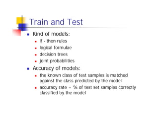
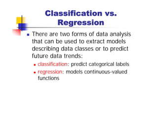
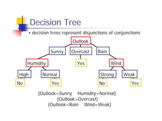
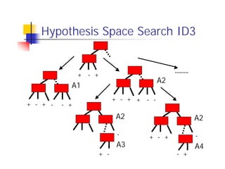
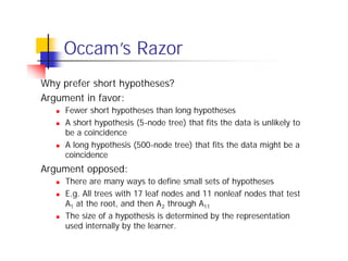
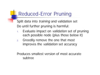
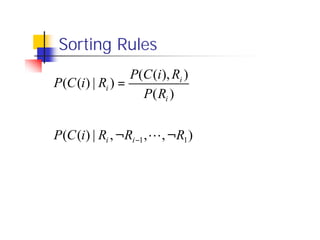
Here are the key steps in ID3's approach to selecting the "best" attribute at each node: 1. Calculate the entropy (impurity/uncertainty) of the target attribute for the examples reaching that node. 2. Calculate the information gain (reduction in entropy) from splitting on each candidate attribute. 3. Select the attribute with the highest information gain. This attribute best separates the examples according to the target class. So in this example, ID3 would calculate the information gain from splitting on attributes A1 and A2, and select the attribute with the highest gain. The goal is to pick the attribute that produces the "purest" partitions at each step.

1. Machine Learning in
Bioinformatics

2. Machine Learning Techniques
n Introduction
n Decision Trees
n Bayesian Methods
n Hidden Markov Models
n Support Vector Machines
n Neural Networks
n Clustering
n Genetic Algorithms
n Association Rules
n Reinforcement Learning
n Fuzzy Sets

3. Software Packages & Datasets
• Weka
• Data Mining Software in Java
• http://www.cs.waikato.ac.nz/~ml/weka
• MLC++
• Machine learning library in C++
• http://www.sig.com/Technology/mlc
• UCI
• Machine Learning Data Repository UC Irvine
• http://www.ics.uci.edu/~mlearn/ML/Repository.html

4. Classification: Definition
n assignment of objects into a set of
predefined categories (classes)
n classification of applicants or patients into
risk levels
n classification of protein sequences into
families
n classification of web pages into topics
n information filter, recommendation, …

5. Classification: Task
n Input: a training set of examples, each
labeled with one class label
n Output: a model (classifier) that assigns a
class label to each instance based on the
other attributes
n The model can be used to predict the
class of new instances, for which the
class label is missing or unknown

6. Patient Risk Prediction
n Given:
n 9714 patient records, each describing a pregnancy
and birth
n Each patient record contains 215 features
n Learn to predict:
n Classes of future patients at high risk for
Emergency Cesarean Section

7. Data Mining Result
One of 18 learned rules:
If No previous vaginal delivery, and
Abnormal 2nd Trimester Ultrasound, and
Malpresentation at admission
Then Probability of Emergency C-Section is 0.6
n Over training data: 26/41 = .63,
n Over test data: 12/20 = .60

8. Train and Test
n example =instance + class label
n Examples are divided into training set +
test set
n Classification model is built in two steps:
n training - build the model from the training
set
n test - check the accuracy of the model
using test set

9. Train and Test
n Kind of models:
n if - then rules
n logical formulae
n decision trees
n joint probabilities
n Accuracy of models:
n the known class of test samples is matched
against the class predicted by the model
n accuracy rate = % of test set samples correctly
classified by the model

10. Training step
Classification
algorithm
training
data
Classifier
Age Car Type Risk
20 Combi High (model)
18 Sports High
40 Sports High
50 Family Low if age < 31
35 Minivan Low
30 Combi High or Car Type =Sports
32 Family Low then Risk = High
14 4 class
2 3
40 Combi Low
attribute label

11. Test step
Classifier
(model)
test
data
Age Car Type Risk Risk
27 Sports High High
34 Family Low Low
66 Family High Low
44 Sports High High

12. Classification (prediction)
Classifier
(model)
new
data
Age Car Type Risk Risk
27 Sports High
34 Minivan Low
55 Family Low
34 Sports High

13. Classification vs.
Regression
n There are two forms of data analysis
that can be used to extract models
describing data classes or to predict
future data trends:
n classification: predict categorical labels
n regression: models continuous-valued
functions

14. Comparing Classification
Methods (1)
n Predictive accuracy: this refers to the ability
of the model to correctly predict the class
label of new or previously unseen data
n Speed: this refers to the computation costs
involved in generating and using the model
n Robustness: this is the ability of the model to
make correct predictions given noisy data or
data with missing values

15. Comparing Classification
Methods (2)
n Scalability: this refers to the ability to
construct the model efficiently given large
amount of data
n Interpretability: this refers to the level of
understanding and insight that is provided by
the model
n Simplicity:
n decision tree size
n rule compactness
n Domain-dependent quality indicators

16. Problem formulation
Given records in the database with
class label – find model for each class.
Age Car Type Risk Age < 31
20 Combi High
18 Sports High Car Type
40 Sports High
is sports
50 Family Low
35 Minivan Low High
30 Combi High
32 Family Low
40 Combi Low High Low

17. Decision Trees

18. Outline
n Decision tree representation
n ID3 learning algorithm
n Entropy, information gain
n Overfitting

19. Decision Trees
n A decision tree is a tree structure, where
n each internal node denotes a test on an
attribute,
n each branch represents the outcome of the
test,
n leaf nodes represent classes or class
distributions Age < 31
Y N
Car Type
is sports
High
High Low

20. Decision Tree
n widely used in inductive inference
n for approximating discrete valued
functions
n can be represented as if-then rules for
human readability
n complete hypothesis space
n successfully applied to many applications
n medical diagnosis
n credit risk prediction

21. Training Examples
Day Outlook Temp. Humidity Wind Play Tennis
D1 Sunny Hot High Weak No
D2 Sunny Hot High Strong No
D3 Overcast Hot High Weak Yes
D4 Rain Mild High Weak Yes
D5 Rain Cool Normal Weak Yes
D6 Rain Cool Normal Strong No
D7 Overcast Cool Normal Weak Yes
D8 Sunny Mild High Weak No
D9 Sunny Cold Normal Weak Yes
D10 Rain Mild Normal Strong Yes
D11 Sunny Mild Normal Strong Yes
D12 Overcast Mild High Strong Yes
D13 Overcast Hot Normal Weak Yes
D14 Rain Mild High Strong No

22. Decision Tree for PlayTennis
Outlook
Sunny Overcast Rain
Humidity Yes Wind
High Normal Strong Weak
No Yes No Yes

23. Decision Tree for C-Section
Risk Prediction
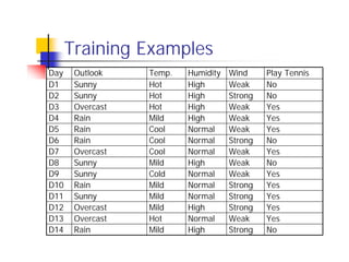
n Learned from medical records of 100 women
[833+,167-] .83+ .17-
Fetal_Presentation = 1: [822+,116-] .88+ .12-
| Previous_Csection = 0: [767+,81-] .90+ .10-
| | Primiparous = 0: [399+,13-] .97+ .03-
| | Primiparous = 1: [368+,68-] .84+ .16-
| | | Fetal_Distress = 0: [334+,47-] .88+ .12-
| | | | Birth_Weight < 3349: [201+,10.6 -] .95+ .05-
| | | | Birth_Weight >= 3349: [133+,36.4 -] .78+ .22-
| | | Fetal_Distress = 1: [34+,21-] .62+ .38-
| Previous_Csection = 1: [55+,35-] .61+ .39-
Fetal_Presentation = 2: [3+,29-] .11+ .89-
Fetal_Presentation = 3: [8+,22-] .27+ .73-

24. Decision Tree for PlayTennis
Outlook
Sunny Overcast Rain
Humidity Each internal node tests an attribute
High Normal Each branch corresponds to an
attribute value node
No Yes Each leaf node assigns a classification

25. Decision Tree for PlayTennis
Outlook Temperature Humidity Wind PlayTennis
Sunny Hot High Weak ?No
Outlook
Sunny Overcast Rain
Humidity Yes Wind
High Normal Strong Weak
No Yes No Yes

26. Decision Tree
• decision trees represent disjunctions of conjunctions
Outlook
Sunny Overcast Rain
Humidity Yes Wind
High Normal Strong Weak
No Yes No Yes
(Outlook=Sunny ∧ Humidity=Normal)
∨ (Outlook=Overcast)
∨ (Outlook=Rain ∧ Wind=Weak)

27. When to consider Decision
Trees
n Instances describable by attribute-value pairs
n Target function is discrete valued
n Disjunctive hypothesis may be required
n Possibly noisy training data
n Missing attribute values
n Examples:
n Medical diagnosis
n Credit risk analysis
n Object classification for robot manipulator (Tan 1993)

28. Top-Down Induction of
Decision Trees ID3
1. A ← the “best” decision attribute for next node
2. Assign A as decision attribute for node
3. For each value of A create new descendant
4. Sort training examples to leaf node according to
the attribute value of the branch
5. If all training examples are perfectly classified
(same value of target attribute) stop, else
iterate over new leaf nodes.

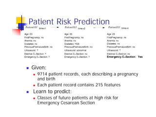
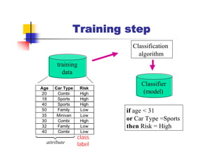
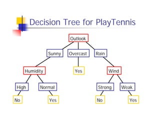
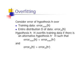
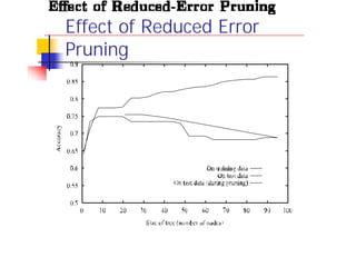
29. Which Attribute is ”best”?
[29+,35-] A1=? A2=? [29+,35-]
True False True False
[21+, 5-] [8+, 30-] [18+, 33-] [11+, 2-]

30. Entropy
n S is a sample of training examples
n p+ is the proportion of positive examples
n p- is the proportion of negative examples
n Entropy measures the impurity of S
Entropy(S) = -p+ log2 p+ - p- log2 p-

31. Entropy
n Entropy(S)= expected number of bits needed to
encode class (+ or -) of randomly drawn
members of S (under the optimal, shortest
length-code)
Why?
n Information theory optimal length code assign
–log2 p bits to messages having probability p.
n So the expected number of bits to encode
(+ or -) of random member of S:
-p+ log2 p+ - p- log2 p-

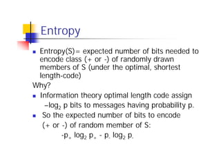
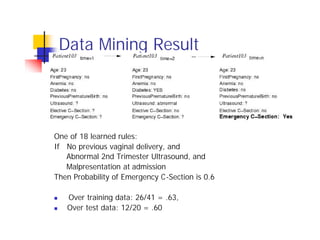
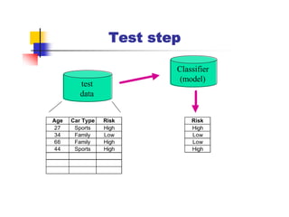
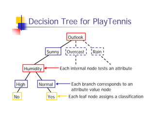
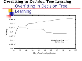
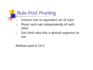
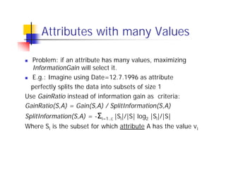
32. Information Gain
n Gain(S,A): expected reduction in entropy due
to sorting S on attribute A
Gain(S,A)=Entropy(S) - ∑v∈values(A) |Sv|/|S| Entropy(Sv)
Entropy([29+,35-]) = -29/64 log2 29/64 – 35/64 log2 35/64
= 0.99
[29+,35-] A1=? A2=? [29+,35-]
True False True False
[21+, 5-] [8+, 30-] [18+, 33-] [11+, 2-]

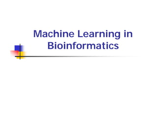
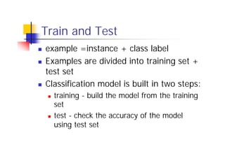
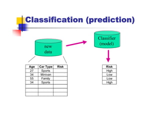
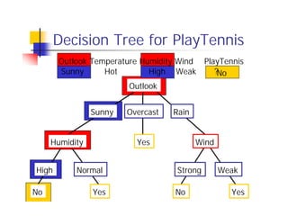
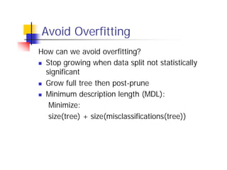
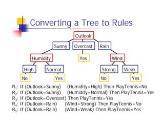
33. Information Gain
Entropy([21+,5-]) = 0.71 Entropy([18+,33-]) = 0.94
Entropy([8+,30-]) = 0.74 Entropy([8+,30-]) = 0.62
Gain(S,A1)=Entropy(S) Gain(S,A2)=Entropy(S)
-26/64*Entropy([21+,5-]) -51/64*Entropy([18+,33-])
-38/64*Entropy([8+,30-]) -13/64*Entropy([11+,2-])
=0.27 =0.12
[29+,35-] A1=? A2=? [29+,35-]
True False True False
[21+, 5-] [8+, 30-] [18+, 33-] [11+, 2-]

34. Training Examples
Day Outlook Temp. Humidity Wind Play Tennis
D1 Sunny Hot High Weak No
D2 Sunny Hot High Strong No
D3 Overcast Hot High Weak Yes
D4 Rain Mild High Weak Yes
D5 Rain Cool Normal Weak Yes
D6 Rain Cool Normal Strong No
D7 Overcast Cool Normal Weak Yes
D8 Sunny Mild High Weak No
D9 Sunny Cold Normal Weak Yes
D10 Rain Mild Normal Strong Yes
D11 Sunny Mild Normal Strong Yes
D12 Overcast Mild High Strong Yes
D13 Overcast Hot Normal Weak Yes
D14 Rain Mild High Strong No

35. Selecting the Next Attribute
S=[9+,5-] S=[9+,5-]
E=0.940 E=0.940
Humidity Wind
High Normal Weak Strong
[3+, 4-] [6+, 1-] [6+, 2-] [3+, 3-]
E=0.985 E=0.592 E=0.811 E=1.0
Gain(S,Humidity) Gain(S,Wind)
=0.940-(7/14)*0.985 =0.940-(8/14)*0.811
– (7/14)*0.592 – (6/14)*1.0
=0.151 =0.048

36. Selecting the Next Attribute
S=[9+,5-]
E=0.940
Outlook
Over
Sunny Rain
cast
[2+, 3-] [4+, 0] [3+, 2-]
E=0.971 E=0.0 E=0.971
Gain(S,Outlook)
=0.940-(5/14)*0.971
-(4/14)*0.0 – (5/14)*0.0971
=0.247

37. ID3 Algorithm
[D1,D2,… ,D14] Outlook
[9+,5-]
Sunny Overcast Rain
Ssunny=[D1,D2,D8,D9,D11] [D3,D7,D12,D13] [D4,D5,D6,D10,D14]
[2+,3-] [4+,0-] [3+,2-]
? Yes ?
Gain(Ssunny , Humidity)=0.970-(3/5)0.0 – 2/5(0.0) = 0.970
Gain(Ssunny , Temp.)=0.970-(2/5)0.0 –2/5(1.0)-(1/5)0.0 = 0.570
Gain(Ssunny , Wind)=0.970= -(2/5)1.0 – 3/5(0.918) = 0.019

38. ID3 Algorithm
Outlook
Sunny Overcast Rain
Humidity Yes Wind
[D3,D7,D12,D13]
High Normal Strong Weak
No Yes No Yes
[D1,D2] [D8,D9,D11] [D6,D14] [D4,D5,D10]

39. Hypothesis Space Search ID3
+ - +
A2
A1
+ - + + - -
+ - + - - +
A2 A2
- + - + -
A3 A4
+ - - +

40. Hypothesis Space Search ID3
n Hypothesis space is complete!
n Target function surely in there…
n Outputs a single hypothesis
n No backtracking on selected attributes (greedy search)
n Local minimal (suboptimal splits)
n Statistically-based search choices
n Robust to noisy data
n Inductive bias (search bias)
n Prefer shorter trees over longer ones
n Place high information gain attributes close to the root

41. Inductive Bias in ID3
n H is the power set of instances X
n Unbiased ?
n Preference for short trees, and for those with high
information gain attributes near the root
n Greedy approximation of BFS-ID3
n BFS through progressively complex trees to find the shortest
consistent tree.
n Bias is a preference imposed by search strategy for
some hypotheses, rather than a restriction of the
hypothesis space H
n Occam’ razor: prefer the shortest (simplest)
s
hypothesis that fits the data

42. Occam’ Razor
s
Why prefer short hypotheses?
Argument in favor:
n Fewer short hypotheses than long hypotheses
n A short hypothesis (5-node tree) that fits the data is unlikely to
be a coincidence
n A long hypothesis (500-node tree) that fits the data might be a
coincidence
Argument opposed:
n There are many ways to define small sets of hypotheses
n E.g. All trees with 17 leaf nodes and 11 nonleaf nodes that test
A1 at the root, and then A 2 through A11
n The size of a hypothesis is determined by the representation
used internally by the learner.

43. Overfitting
Consider error of hypothesis h over
n Training data: error train(h)
n Entire distribution D of data: error D(h)
Hypothesis h∈H overfits training data if there is
∈H
an alternative hypothesis h’ such that
errortrain(h) < errortrain(h’
)
and
errorD(h) > errorD(h’ )

44. Overfitting in Decision Tree
Learning

45. Avoid Overfitting
How can we avoid overfitting?
n Stop growing when data split not statistically
significant
n Grow full tree then post-prune
n Minimum description length (MDL):
Minimize:
size(tree) + size(misclassifications(tree))

46. Reduced-Error Pruning
Split data into training and validation set
Do until further pruning is harmful:
1. Evaluate impact on validation set of pruning
each possible node (plus those below it)
2. Greedily remove the one that most
improves the validation set accuracy
Produces smallest version of most accurate
subtree

47. Effect of Reduced Error
Pruning

48. Rule-Post Pruning
1. Convert tree to equivalent set of rules
2. Prune each rule independently of each
other
3. Sort final rules into a desired sequence to
use
Method used in C4.5

49. Converting a Tree to Rules
Outlook
Sunny Overcast Rain
Humidity Yes Wind
High Normal Strong Weak
No Yes No Yes
R1: If (Outlook=Sunny) ∧ (Humidity=High) Then PlayTennis=No
R2: If (Outlook=Sunny) ∧ (Humidity=Normal) Then PlayTennis=Yes
R3: If (Outlook=Overcast) Then PlayTennis=Yes
R4: If (Outlook=Rain) ∧ (Wind=Strong) Then PlayTennis=No
R5: If (Outlook=Rain) ∧ (Wind=Weak) Then PlayTennis=Yes

50. Sorting Rules
P(C (i ), Ri )
P (C (i ) | Ri ) =
P ( Ri )
P (C (i ) | Ri , ¬Ri −1 , L , ¬R1 )

51. Continuous Valued Attributes
Create a discrete attribute to test continuous
n Temperature = 24.5 0C
n (Temperature > 20.0 0C) = {true, false}
Where to set the threshold?
Temperatur 150C 180C 190C 220C 240C 270C
PlayTennis No No Yes Yes Yes No
(see paper by [Fayyad, Irani 1993]

52. Attributes with many Values
n Problem: if an attribute has many values, maximizing
InformationGain will select it.
n E.g.: Imagine using Date=12.7.1996 as attribute
perfectly splits the data into subsets of size 1
Use GainRatio instead of information gain as criteria:
GainRatio(S,A) = Gain(S,A) / SplitInformation(S,A)
SplitInformation(S,A) = -Σi=1..c |Si|/|S| log2 |Si|/|S|
Where Si is the subset for which attribute A has the value v i

53. Attributes with Cost
Consider:
n Medical diagnosis : blood test costs 1000 SEK
n Robotics: width_from_one_feet has cost 23 secs.
How to learn a consistent tree with low expected
cost?
Replace Gain by :
Gain2(S,A)/Cost(A) [Tan, Schimmer 1990]
2Gain(S,A)-1/(Cost(A)+1)w w ∈[0,1] [Nunez 1988]