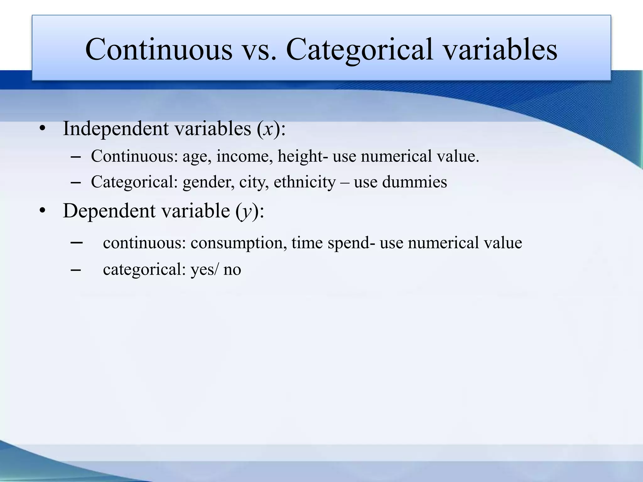
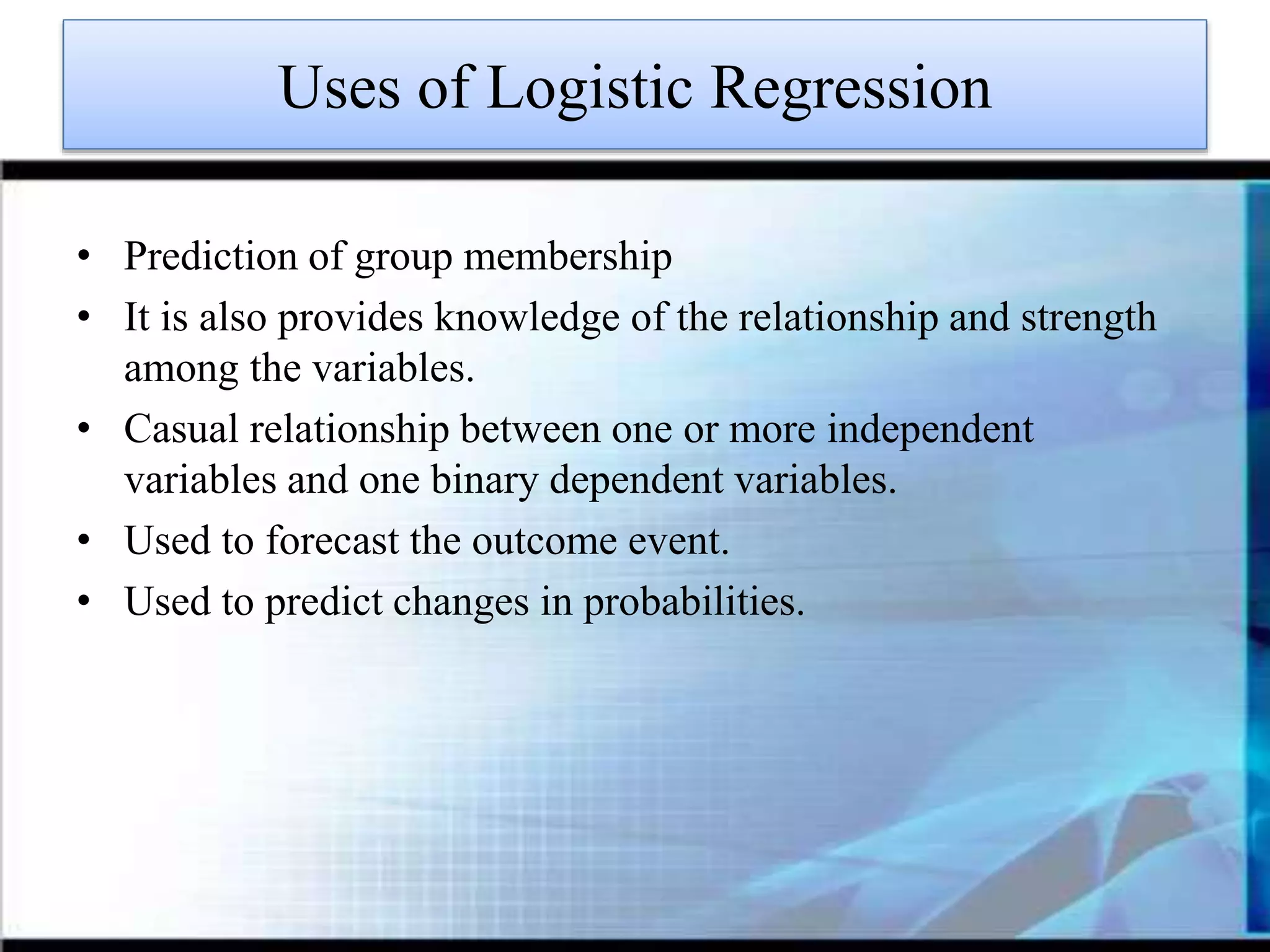
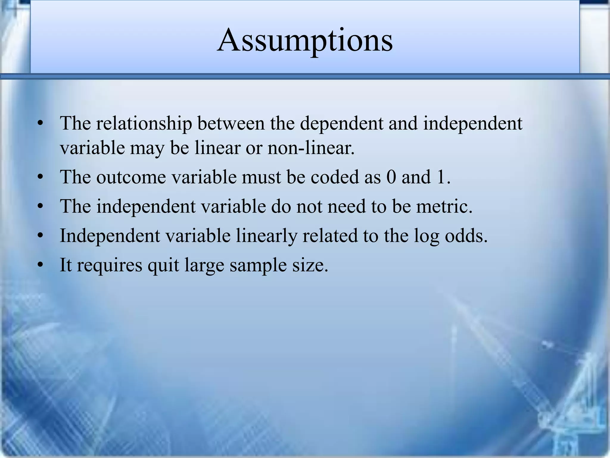
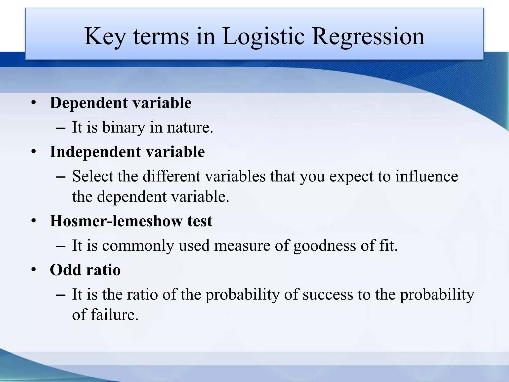
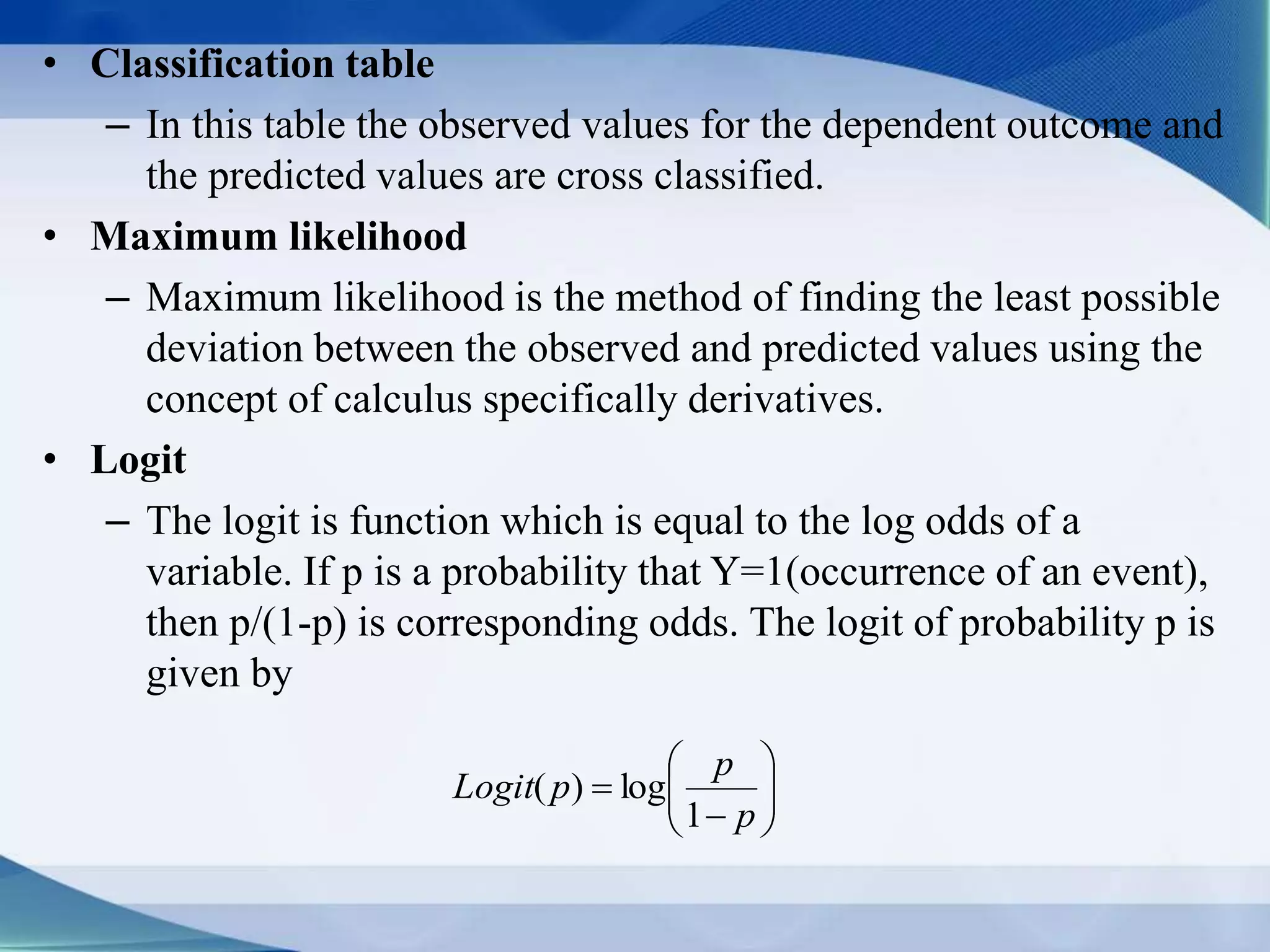
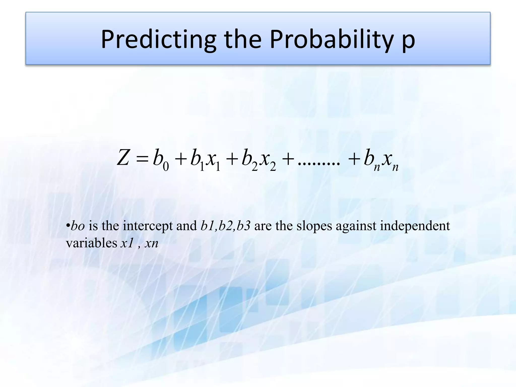
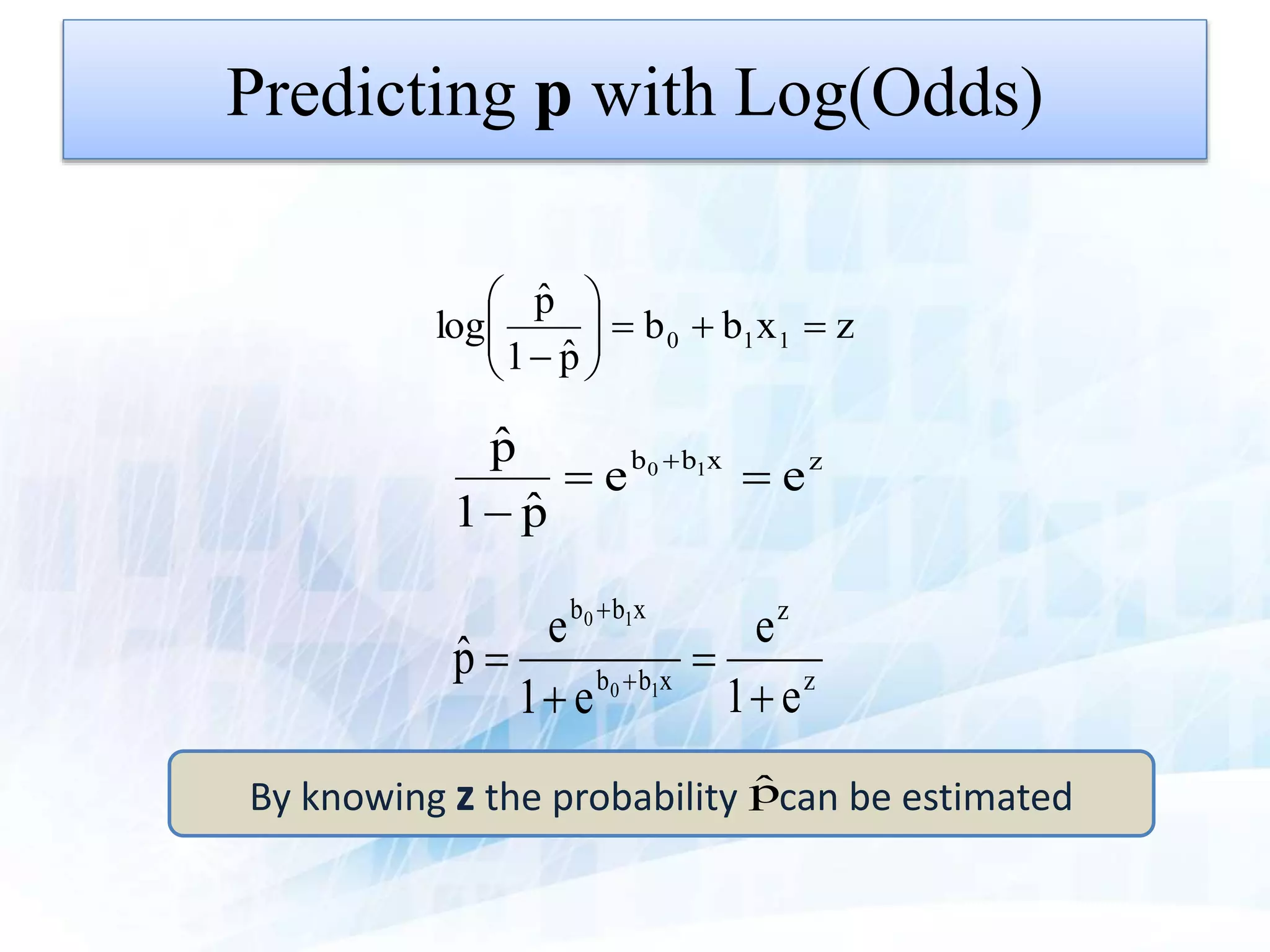
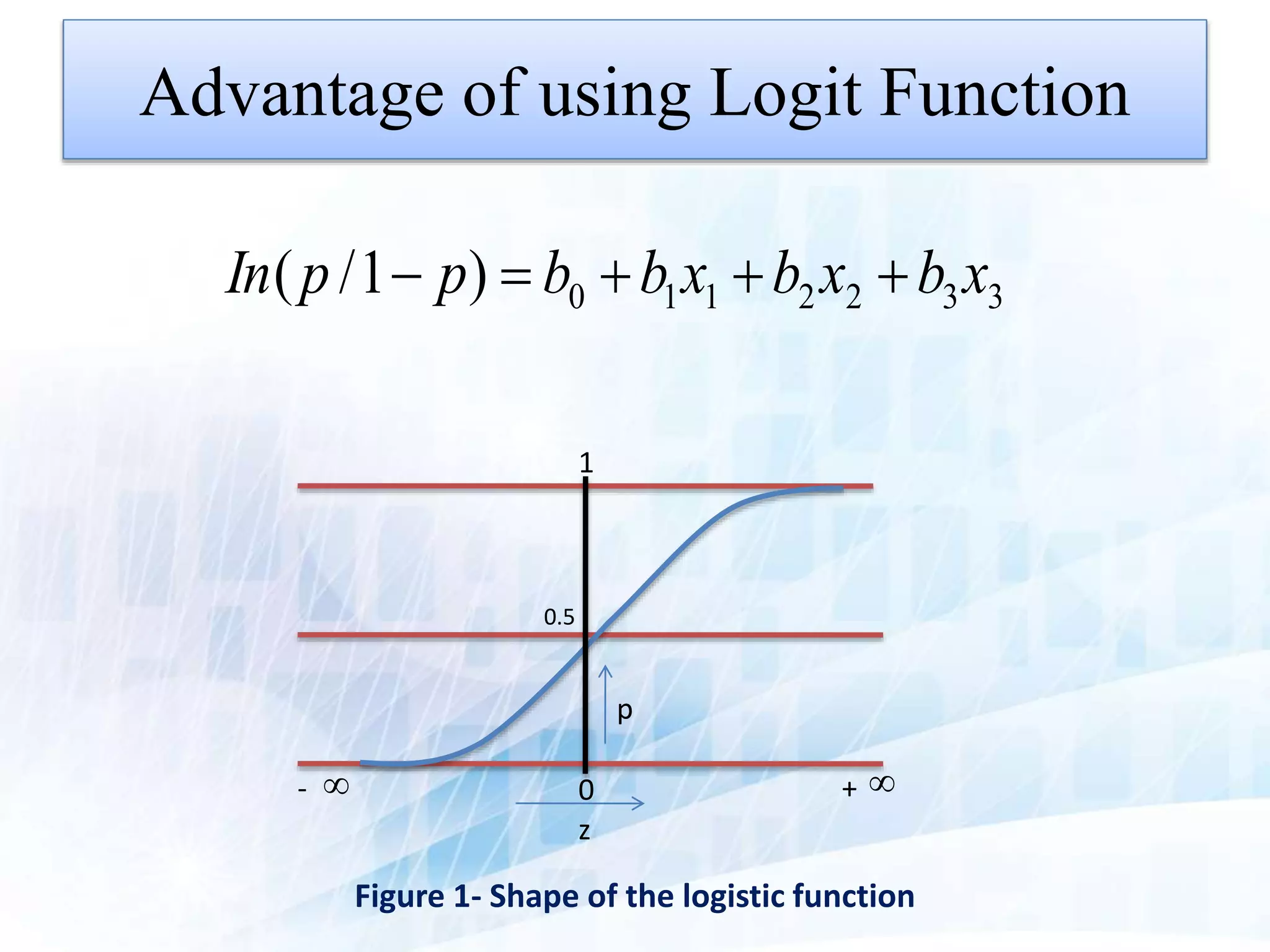
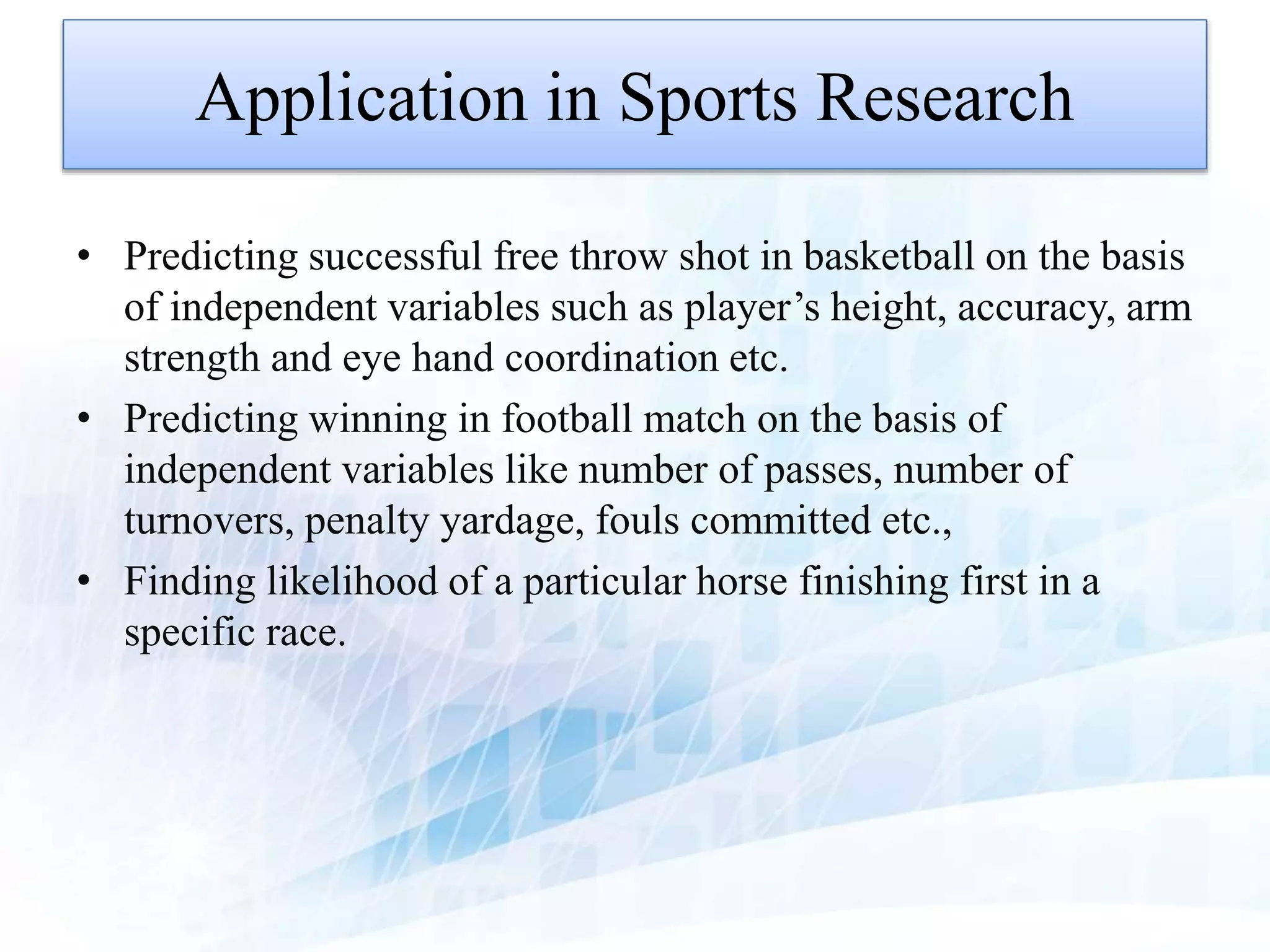
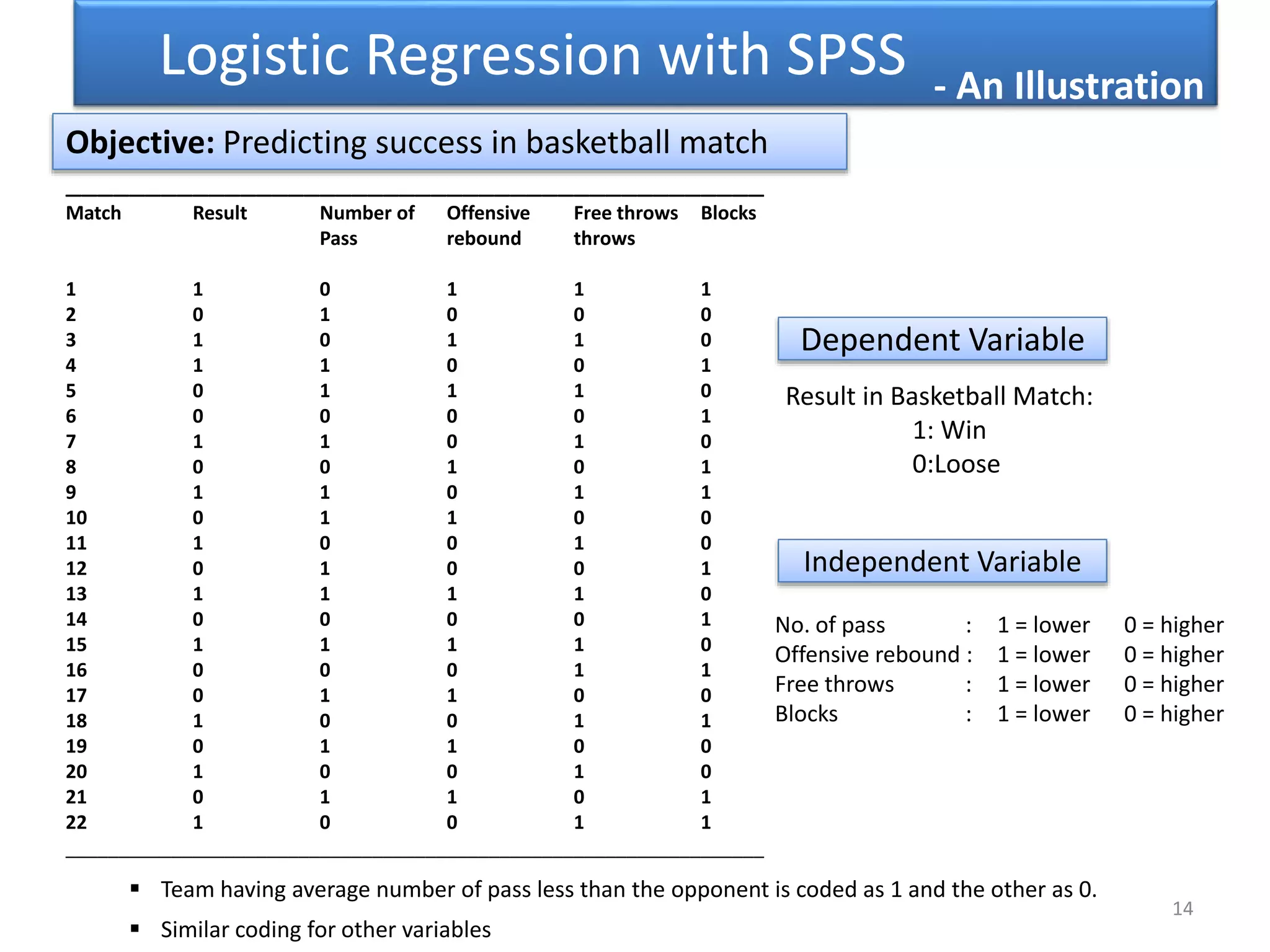
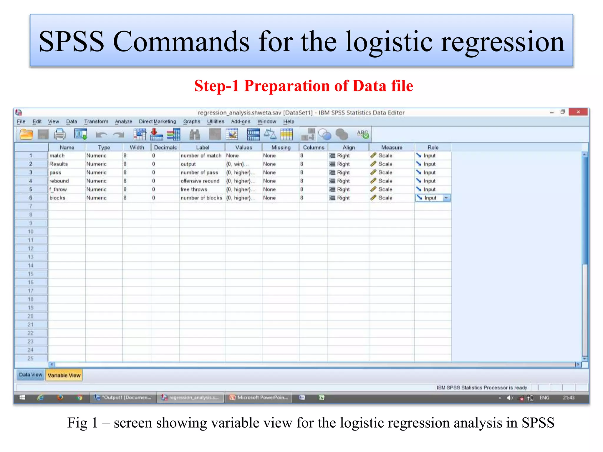
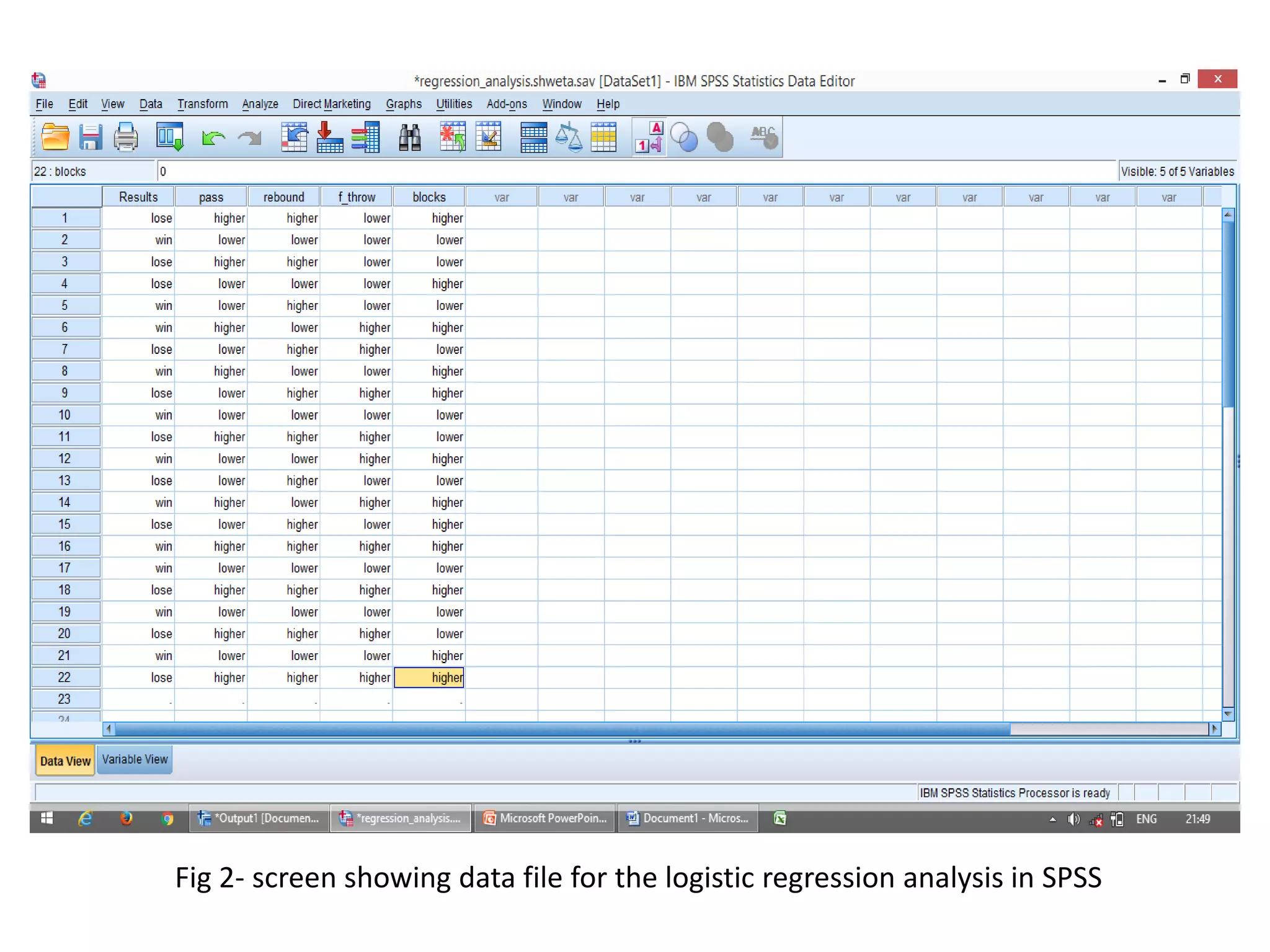
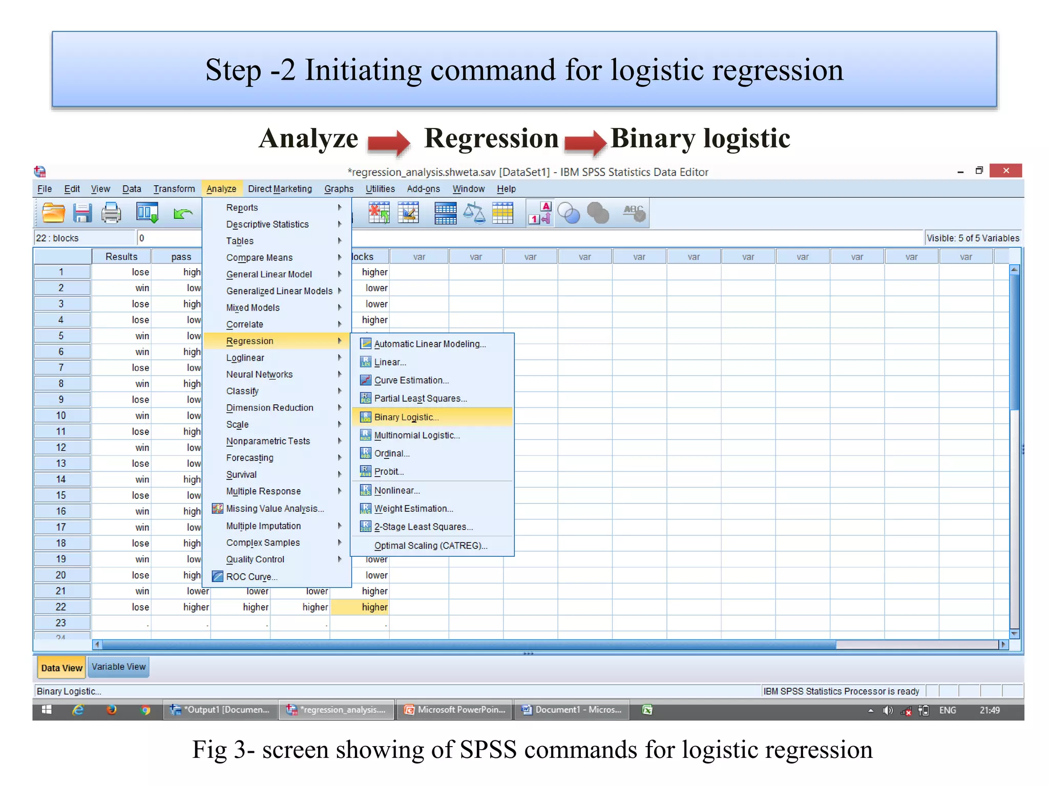
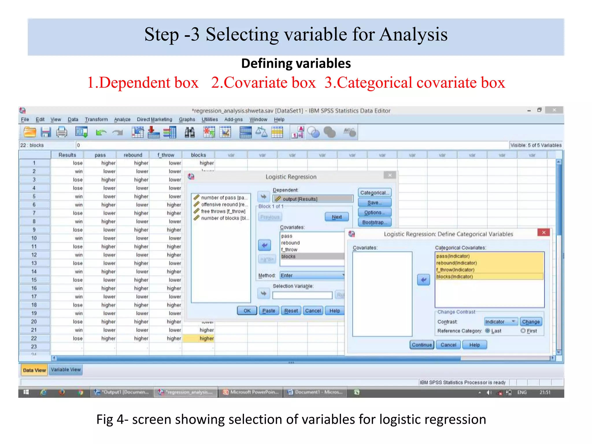
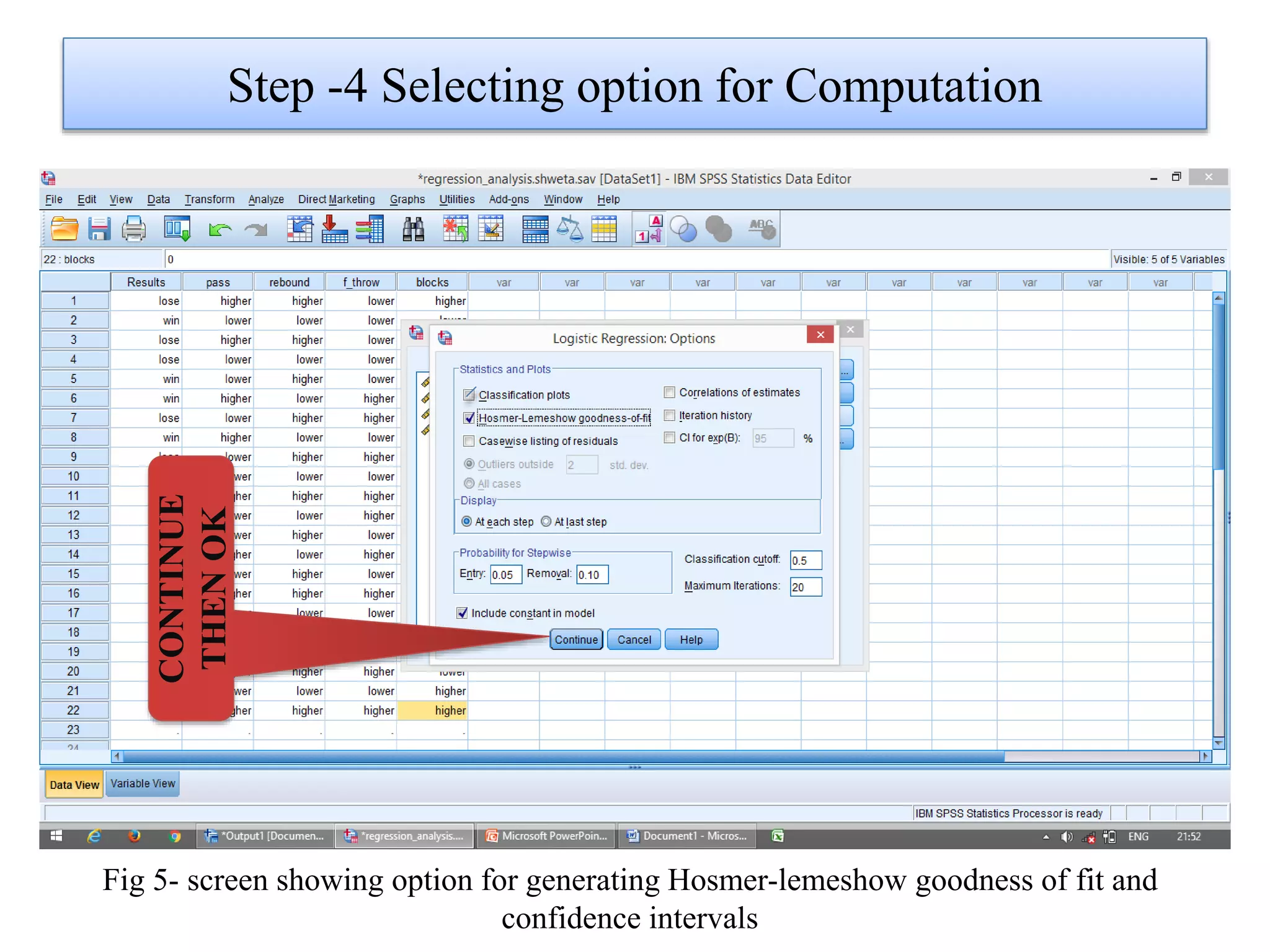
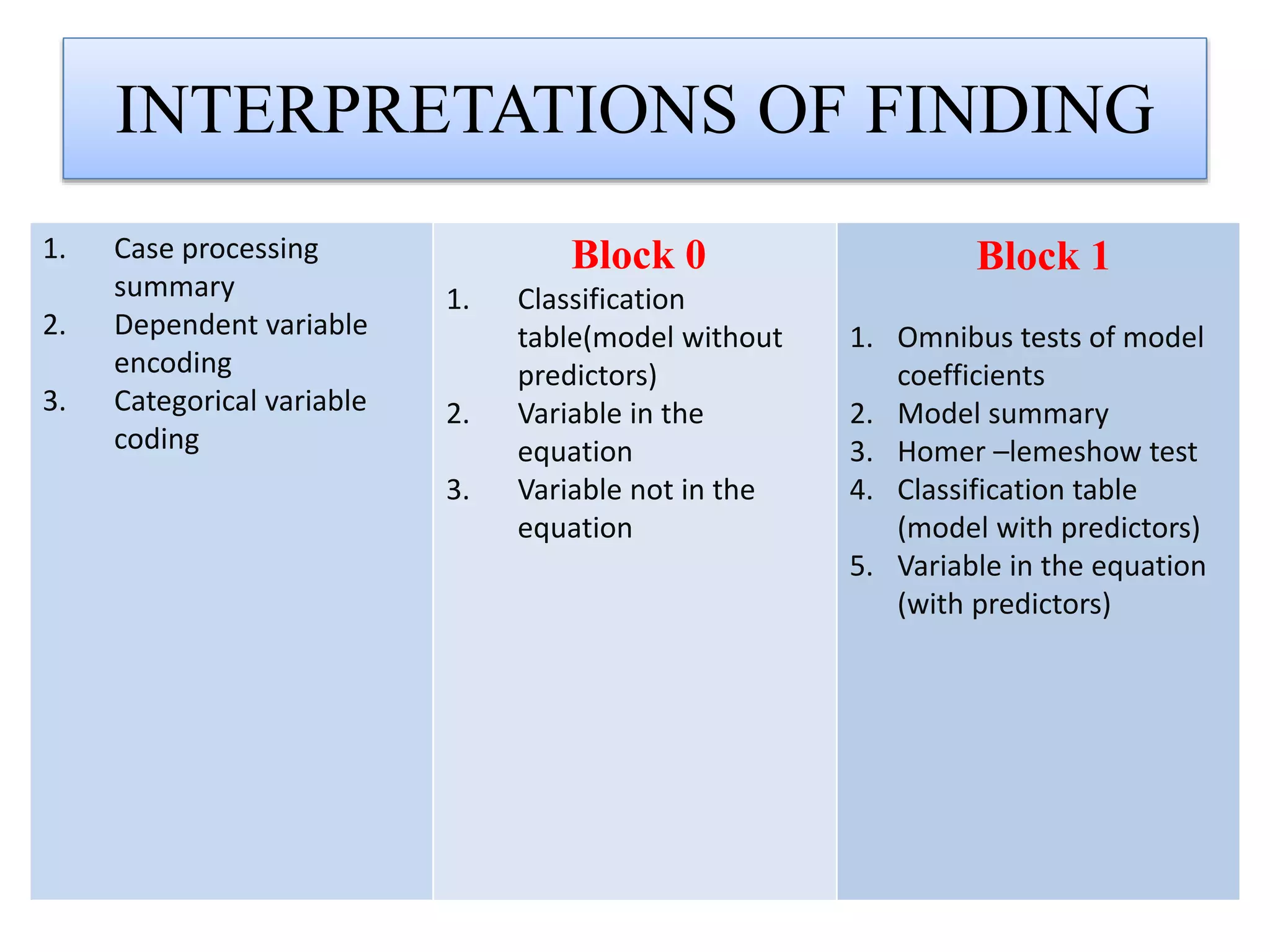
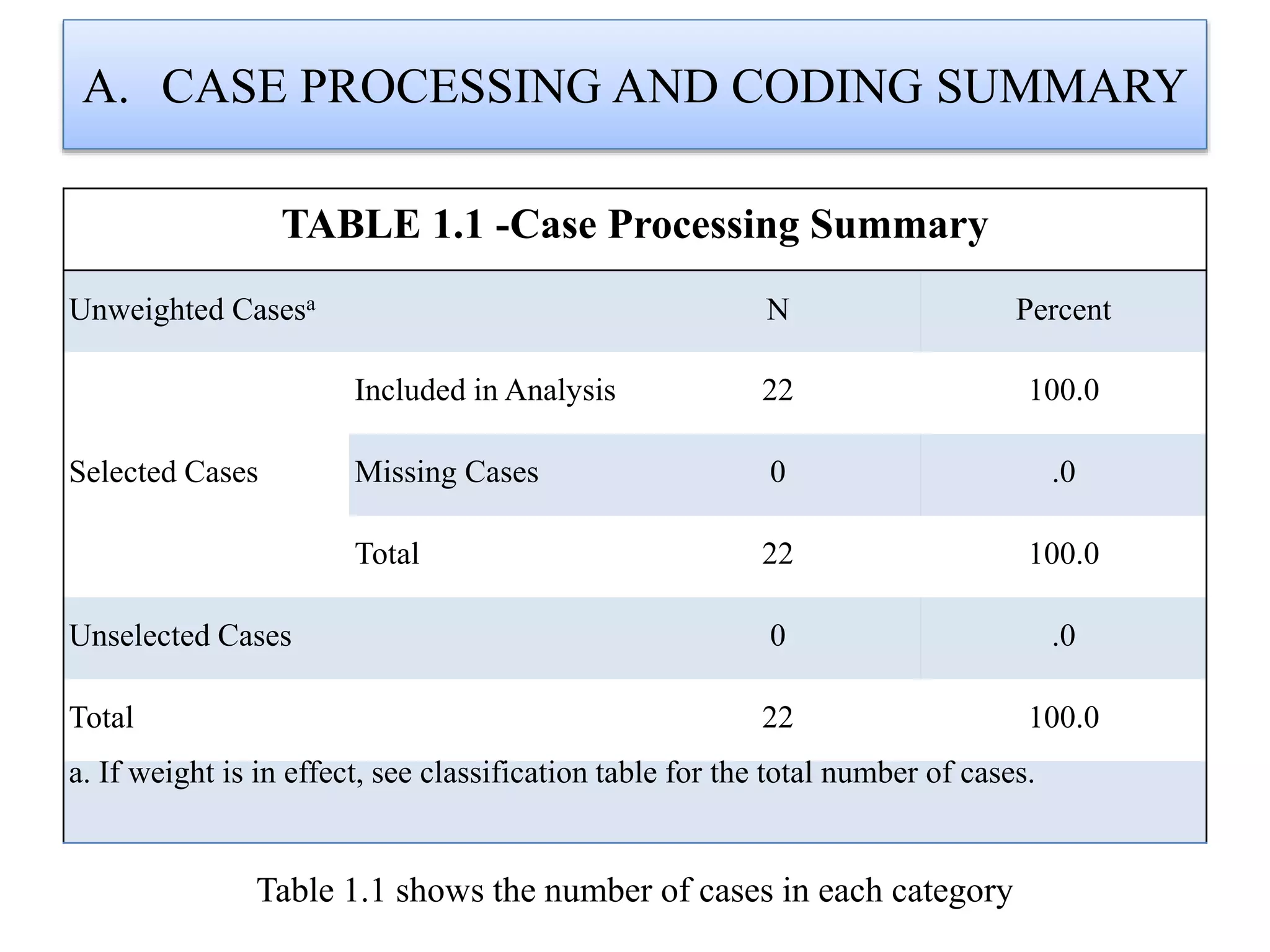
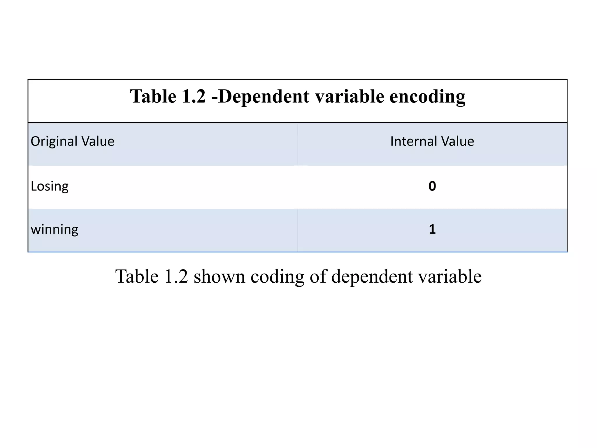
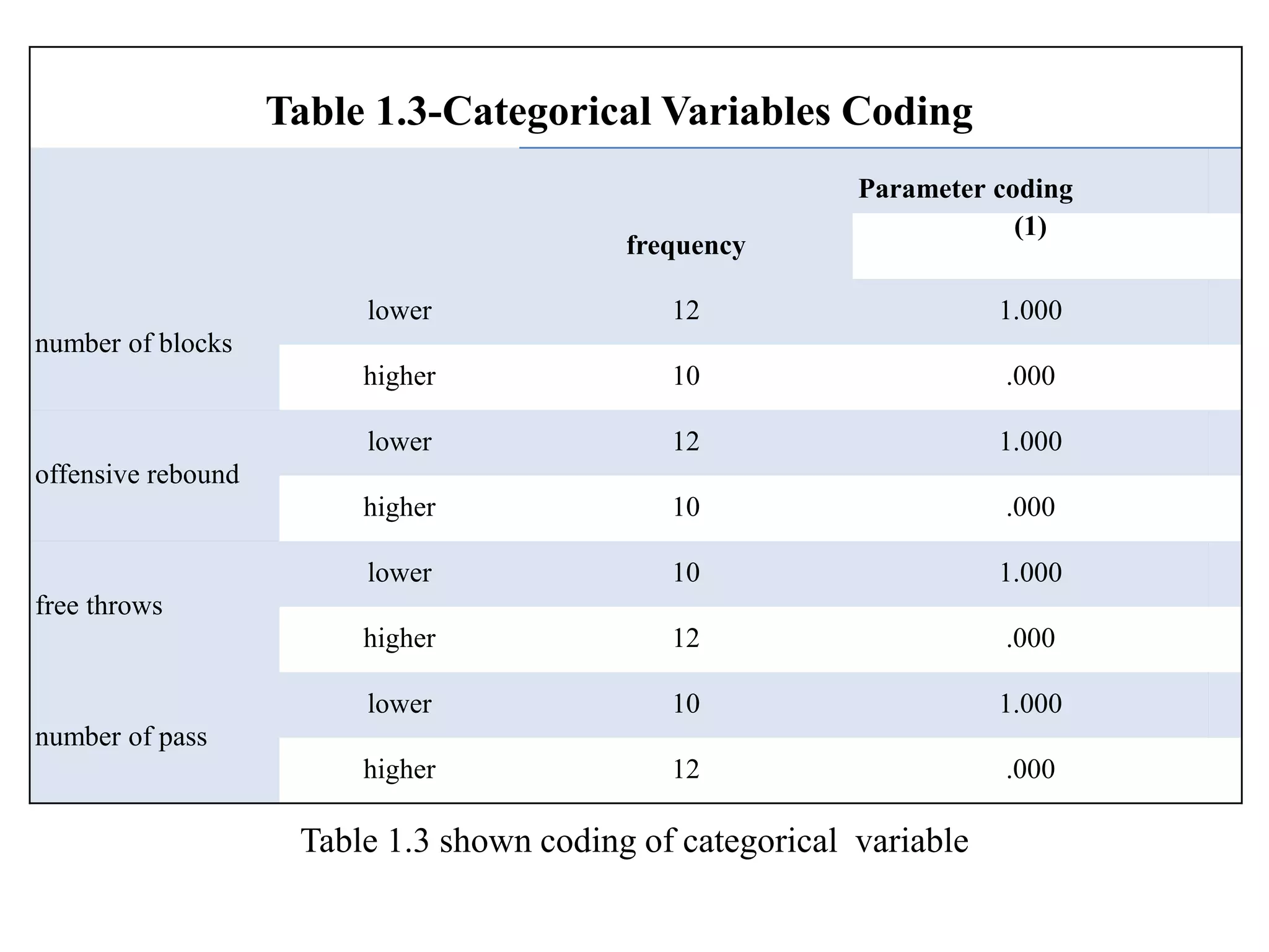
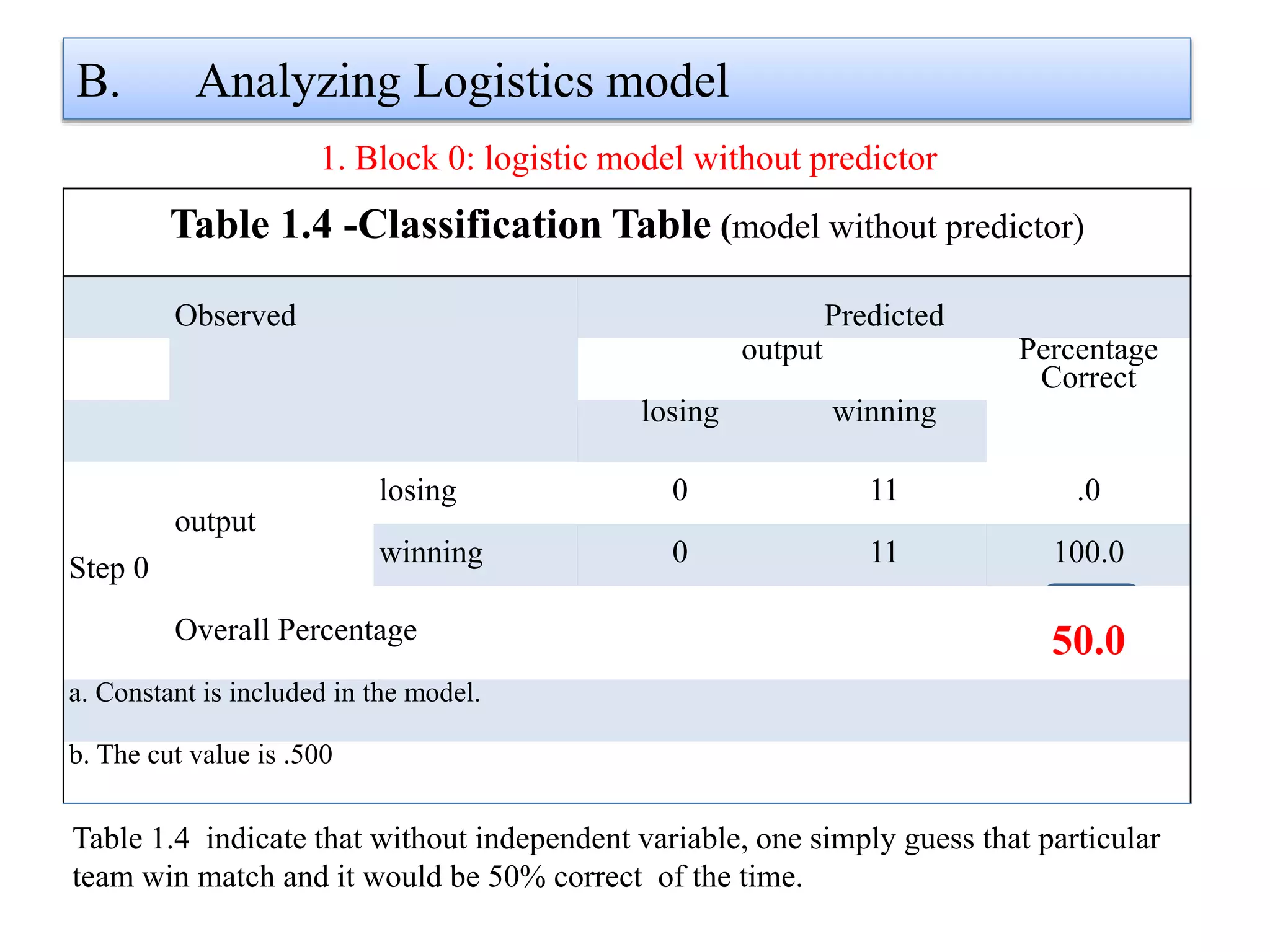
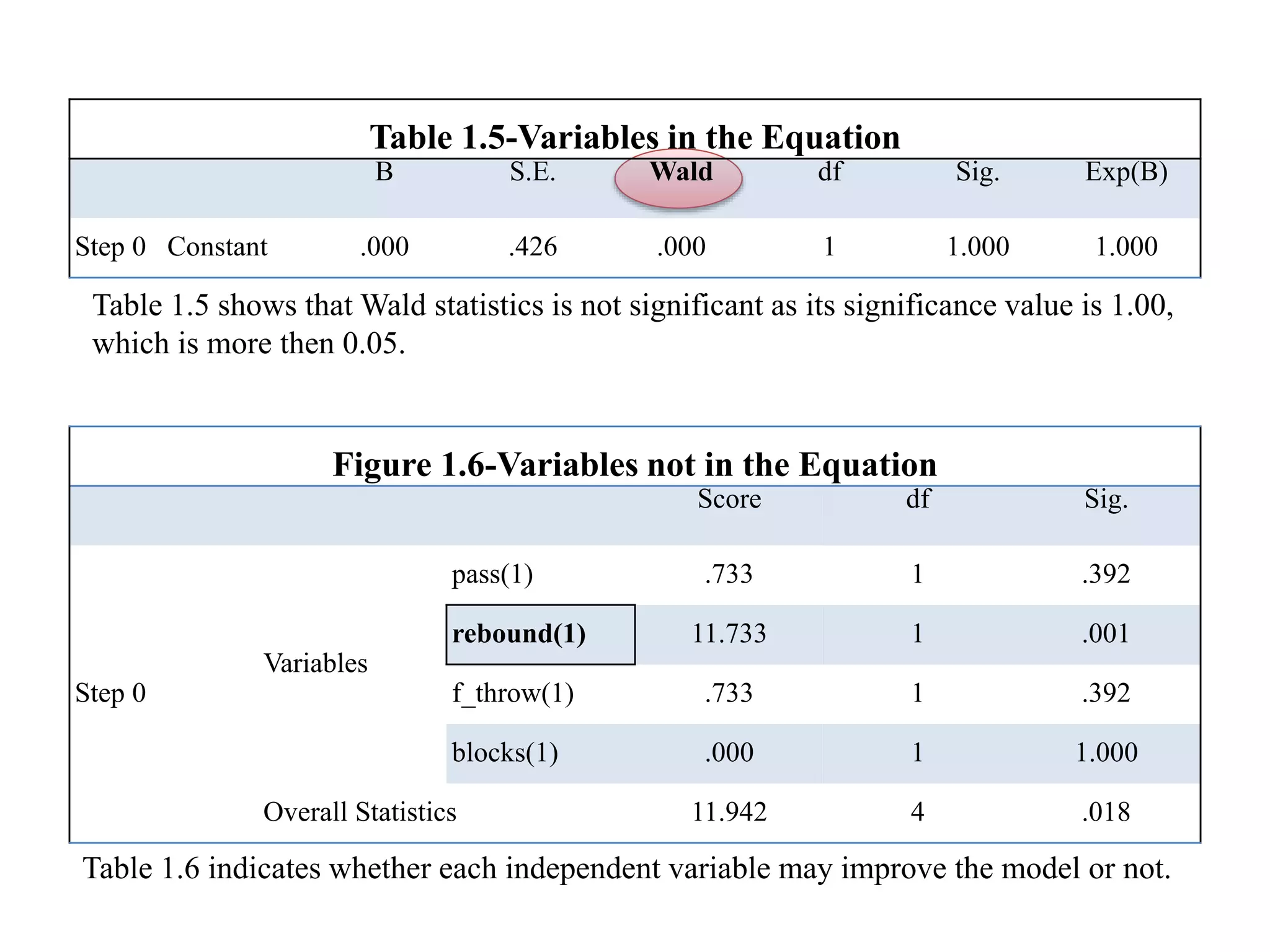
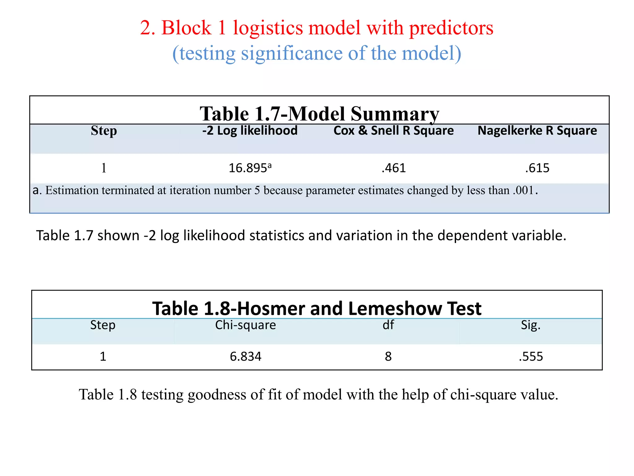
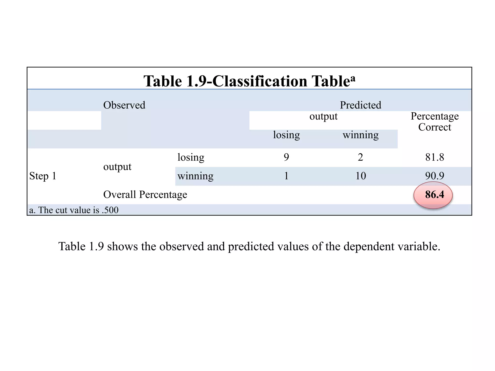
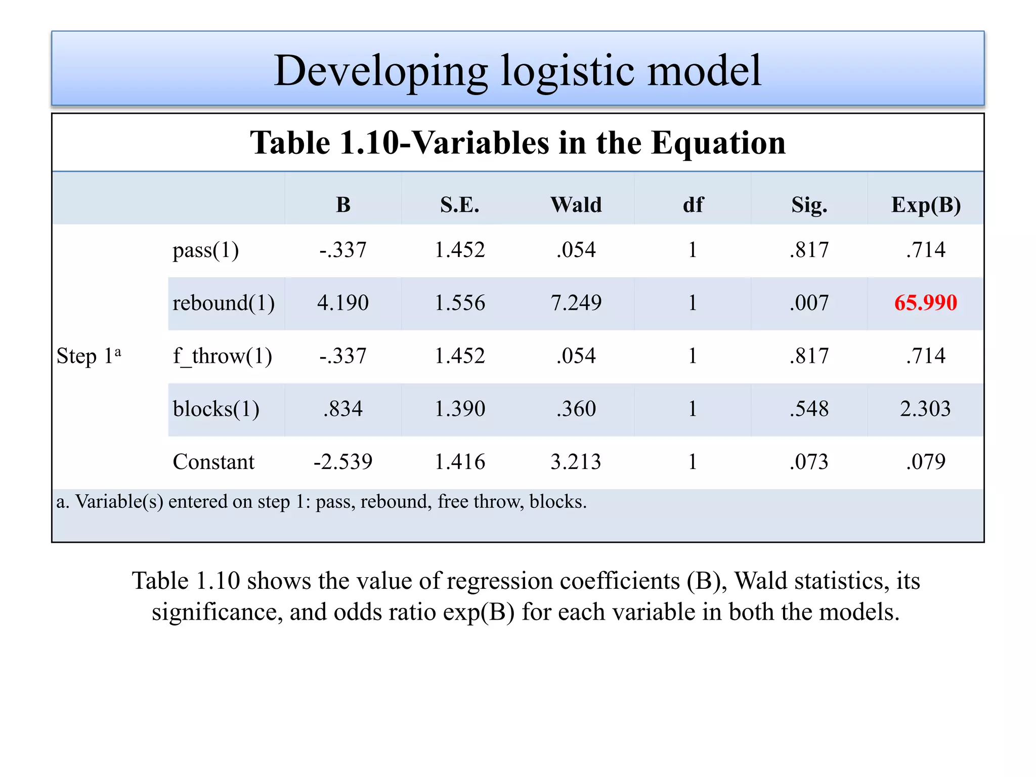
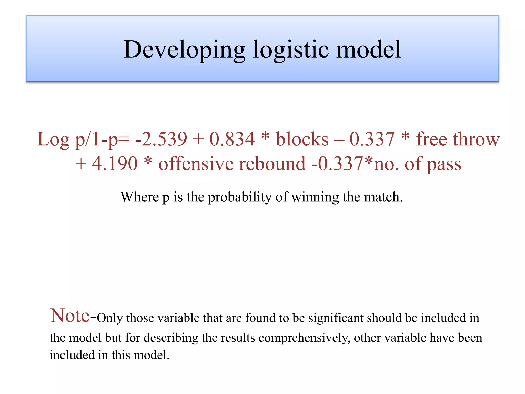
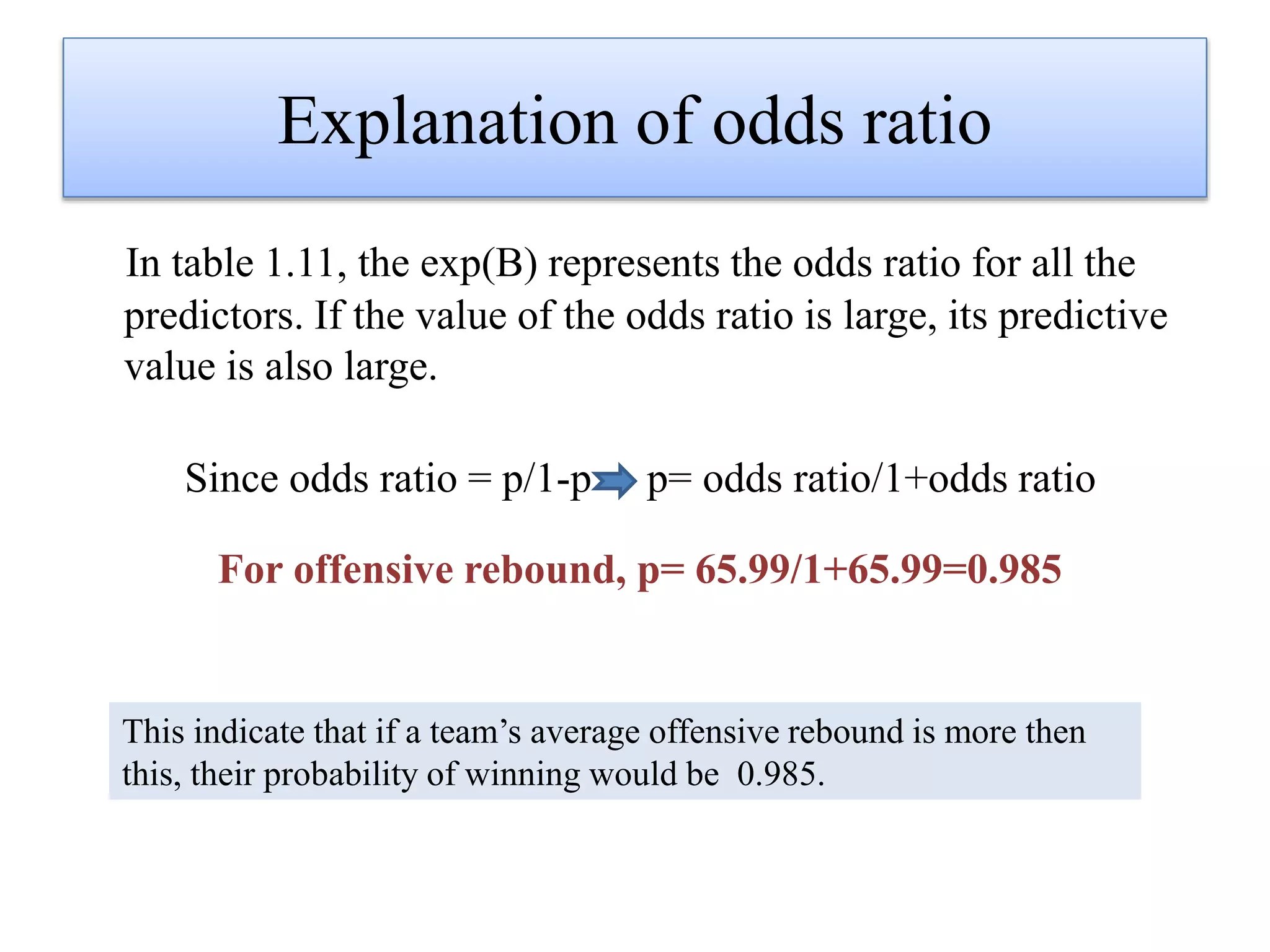
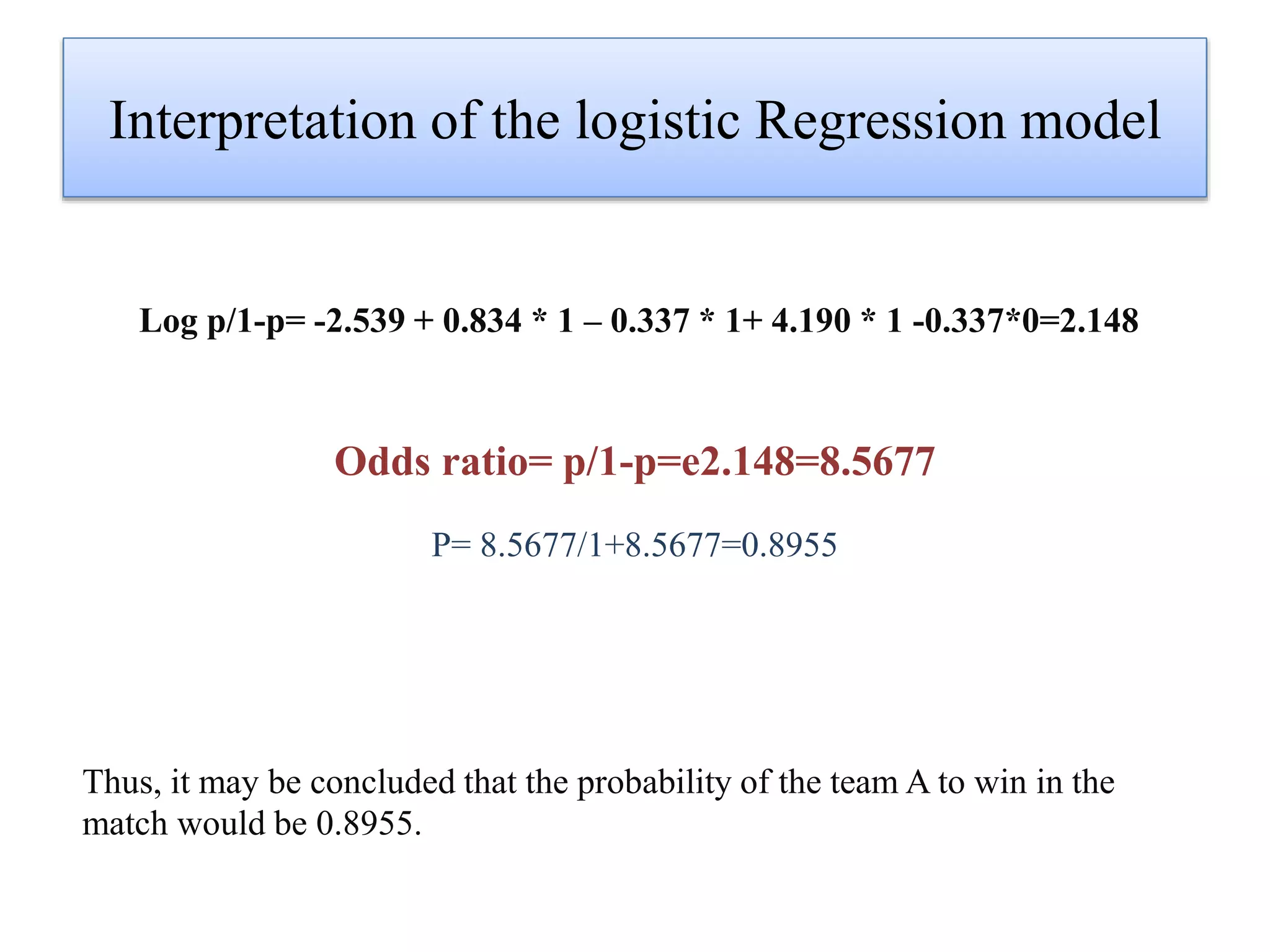
Logistic regression is used to predict categorical outcomes. The presented document discusses logistic regression, including its objectives, assumptions, key terms, and an example application to predicting basketball match outcomes. Logistic regression uses maximum likelihood estimation to model the relationship between a binary dependent variable and independent variables. The document provides an illustrated example of conducting logistic regression in SPSS to predict match results based on variables like passes, rebounds, free throws, and blocks.

1. LOGISTIC REGRESSION
Presented by
Mr. Vijay Singh Rawat
Ms. Shweta
(Research Scholar)
Ph. D
Course work 2017-18
Lakshmibai National Institute of Physical Education, Gwalior, India
(Deemed to be University)

2. INTRODUCTION
• Logistic regression is a predictive analysis.
• Used in a situation when a researcher is interested to predict
the occurrence of any happenings.

3. Objective of Logistic Regression
• The objective of Logistic regression is to find the best fitting
model to describe the relationship between the dichotomous
characteristics of interest and a set of independent variables.

4. Continuous vs. Categorical variables
• Independent variables (x):
– Continuous: age, income, height- use numerical value.
– Categorical: gender, city, ethnicity – use dummies
• Dependent variable (y):
– continuous: consumption, time spend- use numerical value
– categorical: yes/ no

5. Examples of Binary Outcomes
• Should a bank give a person loan or not.
• What determines admittance into a school.
• Which consumers are more likely to buy a new product.

6. Uses of Logistic Regression
• Prediction of group membership
• It is also provides knowledge of the relationship and strength
among the variables.
• Casual relationship between one or more independent
variables and one binary dependent variables.
• Used to forecast the outcome event.
• Used to predict changes in probabilities.

7. Assumptions
• The relationship between the dependent and independent
variable may be linear or non-linear.
• The outcome variable must be coded as 0 and 1.
• The independent variable do not need to be metric.
• Independent variable linearly related to the log odds.
• It requires quit large sample size.

8. Key terms in Logistic Regression
• Dependent variable
– It is binary in nature.
• Independent variable
– Select the different variables that you expect to influence
the dependent variable.
• Hosmer-lemeshow test
– It is commonly used measure of goodness of fit.
• Odd ratio
– It is the ratio of the probability of success to the probability
of failure.

9. • Classification table
– In this table the observed values for the dependent outcome and
the predicted values are cross classified.
• Maximum likelihood
– Maximum likelihood is the method of finding the least possible
deviation between the observed and predicted values using the
concept of calculus specifically derivatives.
• Logit
– The logit is function which is equal to the log odds of a
variable. If p is a probability that Y=1(occurrence of an event),
then p/(1-p) is corresponding odds. The logit of probability p is
given by








p
p
pLogit
1
log)(

10. Predicting the Probability p
nn xbxbxbbZ  .........22110
•bo is the intercept and b1,b2,b3 are the slopes against independent
variables x1 , xn

11. Predicting p with Log(Odds)
zxbb
pˆ1
pˆ
log 110 






zxbb
ee
pˆ1
pˆ 10



z
z
xbb
xbb
e1
e
e1
e
pˆ
10
10



 

By knowing z the probability can be estimatedpˆ

12. Advantage of using Logit Function
3322110)1/( xbxbxbbppIn 
+-
0.5
p
1
z
0
Figure 1- Shape of the logistic function

13. Application in Sports Research
• Predicting successful free throw shot in basketball on the basis
of independent variables such as player’s height, accuracy, arm
strength and eye hand coordination etc.
• Predicting winning in football match on the basis of
independent variables like number of passes, number of
turnovers, penalty yardage, fouls committed etc.,
• Finding likelihood of a particular horse finishing first in a
specific race.

14. Logistic Regression with SPSS
Objective: Predicting success in basketball match
____________________________________________
Match Result Number of Offensive Free throws Blocks
Pass rebound throws
1 1 0 1 1 1
2 0 1 0 0 0
3 1 0 1 1 0
4 1 1 0 0 1
5 0 1 1 1 0
6 0 0 0 0 1
7 1 1 0 1 0
8 0 0 1 0 1
9 1 1 0 1 1
10 0 1 1 0 0
11 1 0 0 1 0
12 0 1 0 0 1
13 1 1 1 1 0
14 0 0 0 0 1
15 1 1 1 1 0
16 0 0 0 1 1
17 0 1 1 0 0
18 1 0 0 1 1
19 0 1 1 0 0
20 1 0 0 1 0
21 0 1 1 0 1
22 1 0 0 1 1
__________________________________________________________________
Dependent Variable
Independent Variable
Result in Basketball Match:
1: Win
0:Loose
No. of pass : 1 = lower 0 = higher
Offensive rebound : 1 = lower 0 = higher
Free throws : 1 = lower 0 = higher
Blocks : 1 = lower 0 = higher
 Team having average number of pass less than the opponent is coded as 1 and the other as 0.
 Similar coding for other variables
- An Illustration
14

15. SPSS Commands for the logistic regression
Step-1 Preparation of Data file
Fig 1 – screen showing variable view for the logistic regression analysis in SPSS

16. Fig 2- screen showing data file for the logistic regression analysis in SPSS

17. Step -2 Initiating command for logistic regression
Fig 3- screen showing of SPSS commands for logistic regression
Analyze Regression Binary logistic

18. Fig 4- screen showing selection of variables for logistic regression
Defining variables
1.Dependent box 2.Covariate box 3.Categorical covariate box
Step -3 Selecting variable for Analysis

19. Step -4 Selecting option for Computation
Fig 5- screen showing option for generating Hosmer-lemeshow goodness of fit and
confidence intervals
CONTINUE
THENOK

20. Step-5 Selecting method for entering independent
variable in logistic regression
A. Confirmatory study
B. Exploratory study
• Clicking the option ok to get the output
Step-6 Getting the output

21. The logistic regression in SPSS is run in two steps
• First step (block 0)
– It includes no predictors and just the intercept.
• Second step (block 1)
– It includes the variable in the analysis and coding of
independent and dependent variable..

22. INTERPRETATIONS OF FINDING
1. Case processing
summary
2. Dependent variable
encoding
3. Categorical variable
coding
Block 0
1. Classification
table(model without
predictors)
2. Variable in the
equation
3. Variable not in the
equation
Block 1
1. Omnibus tests of model
coefficients
2. Model summary
3. Homer –lemeshow test
4. Classification table
(model with predictors)
5. Variable in the equation
(with predictors)

23. A. CASE PROCESSING AND CODING SUMMARY
TABLE 1.1 -Case Processing Summary
Unweighted Casesa N Percent
Selected Cases
Included in Analysis 22 100.0
Missing Cases 0 .0
Total 22 100.0
Unselected Cases 0 .0
Total 22 100.0
a. If weight is in effect, see classification table for the total number of cases.
Table 1.1 shows the number of cases in each category

24. Table 1.2 shown coding of dependent variable
Table 1.2 -Dependent variable encoding
Original Value Internal Value
Losing 0
winning 1

25. Table 1.3-Categorical Variables Coding
frequency
Parameter coding
(1)
number of blocks
lower 12 1.000
higher 10 .000
offensive rebound
lower 12 1.000
higher 10 .000
free throws
lower 10 1.000
higher 12 .000
number of pass
lower 10 1.000
higher 12 .000
Table 1.3 shown coding of categorical variable

26. B. Analyzing Logistics model
Table 1.4 -Classification Table (model without predictor)
Observed Predicted
output Percentage
Correct
losing winning
Step 0
output
losing 0 11 .0
winning 0 11 100.0
Overall Percentage 50.0
a. Constant is included in the model.
b. The cut value is .500
Table 1.4 indicate that without independent variable, one simply guess that particular
team win match and it would be 50% correct of the time.
1. Block 0: logistic model without predictor

27. Table 1.5-Variables in the Equation
B S.E. Wald df Sig. Exp(B)
Step 0 Constant .000 .426 .000 1 1.000 1.000
Figure 1.6-Variables not in the Equation
Score df Sig.
Step 0
Variables
pass(1) .733 1 .392
rebound(1) 11.733 1 .001
f_throw(1) .733 1 .392
blocks(1) .000 1 1.000
Overall Statistics 11.942 4 .018
Table 1.5 shows that Wald statistics is not significant as its significance value is 1.00,
which is more then 0.05.
Table 1.6 indicates whether each independent variable may improve the model or not.

28. 2. Block 1 logistics model with predictors
(testing significance of the model)
Table 1.7-Model Summary
Step -2 Log likelihood Cox & Snell R Square Nagelkerke R Square
1 16.895a .461 .615
a. Estimation terminated at iteration number 5 because parameter estimates changed by less than .001.
Table 1.7 shown -2 log likelihood statistics and variation in the dependent variable.
Table 1.8-Hosmer and Lemeshow Test
Step Chi-square df Sig.
1 6.834 8 .555
Table 1.8 testing goodness of fit of model with the help of chi-square value.

29. Table 1.9-Classification Tablea
Observed Predicted
output Percentage
Correct
losing winning
Step 1
output
losing 9 2 81.8
winning 1 10 90.9
Overall Percentage 86.4
a. The cut value is .500
Table 1.9 shows the observed and predicted values of the dependent variable.

30. Developing logistic model
Table 1.10-Variables in the Equation
B S.E. Wald df Sig. Exp(B)
Step 1a
pass(1) -.337 1.452 .054 1 .817 .714
rebound(1) 4.190 1.556 7.249 1 .007 65.990
f_throw(1) -.337 1.452 .054 1 .817 .714
blocks(1) .834 1.390 .360 1 .548 2.303
Constant -2.539 1.416 3.213 1 .073 .079
a. Variable(s) entered on step 1: pass, rebound, free throw, blocks.
Table 1.10 shows the value of regression coefficients (B), Wald statistics, its
significance, and odds ratio exp(B) for each variable in both the models.

31. Developing logistic model
Where p is the probability of winning the match.
Note-Only those variable that are found to be significant should be included in
the model but for describing the results comprehensively, other variable have been
included in this model.
Log p/1-p= -2.539 + 0.834 * blocks – 0.337 * free throw
+ 4.190 * offensive rebound -0.337*no. of pass

32. Explanation of odds ratio
In table 1.11, the exp(B) represents the odds ratio for all the
predictors. If the value of the odds ratio is large, its predictive
value is also large.
Since odds ratio = p/1-p = p= odds ratio/1+odds ratio
For offensive rebound, p= 65.99/1+65.99=0.985
This indicate that if a team’s average offensive rebound is more then
this, their probability of winning would be 0.985.

33. Interpretation of the logistic Regression model
Log p/1-p= -2.539 + 0.834 * 1 – 0.337 * 1+ 4.190 * 1 -0.337*0=2.148
Odds ratio= p/1-p=e2.148=8.5677
P= 8.5677/1+8.5677=0.8955
Thus, it may be concluded that the probability of the team A to win in the
match would be 0.8955.

34. s