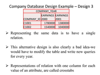
RDBMS - Unit II
Chapter 7
Relational Database Design
Prepared By
Dr. S.Murugan, Associate Professor
Department of Computer Science,
AlagappaGovernment Arts College, Karaikudi.
(Affiliated by AlagappaUniversity)
Mailid: muruganjit@gmail.com
Reference Book:
Database System Concepts by Abraham Silberschatz, Henry
F.Korth , S. Sudharshan
7.1 Features of Good Relational Database Design
➢ The goal of a relational database design is to generate a set of
relation schemas which is used to store information without
unnecessary redundancy.
7.1.1 Design Alternative: Larger Schema
➢ The database design for maintaining a loan details are look like
as follows:
➢ Good Database Design (Less Data Redundancy)
➢ Borrower = (customer_id, loan_number)
➢ loan=(loan_number, amount)
➢ The above database design may be re-designed (natural join of
borrower and loan) as follows
➢ Bad Database Design (High Data Redundancy)
➢ Bor_loan= (customer_id, loan_number, amount)
7.1.1 Design Alternative 1: Larger Schema
➢ Three customers may avail the single loan amount Rs.10000
with the loan number L-100.
➢ In bor_loan relation, the value of loan number and amount is
repeated.
➢ In loan and borrower relation, the amount of each loan exactly
once.
7.1.1 Design Alternative 2: Larger Schema
➢ Another alternative design loan_amt_branch is derived from
loan and loan_branch.
7.1.2 Design Alternative: Smaller Schemas
➢ An Employee relation may be decomposed into two relation.
➢ If the resultant of natural join of the decomposed relation is
similar to the original relation then the decomposed relational
database design is good decomposition. Otherwise bad Database
decomposition.
➢ In the fig. 7.4, the original relation and the result of natural join
is not similar. i.e., Loss of information. (The start date of the
natural join is repeated and it is meaningless)
➢ In Fig, 7.2 and 7.3 there is no loss of information.
7.1.2 Design Alternative: Smaller Schemas
7.2 Atomic Domains and First Normal Form
➢ A relation schema R is in first normal form (1NF) if
the domains of all attributes of R are atomic.
➢ A domain is atomic if elements of the domain are
considered to be indivisible units.
➢ A domain is non-atomic if elements of the domain are
considered to be divisible units.
➢ Example for atomic domain: Age, Rollnumber
➢ Example for non-atomic domain : Address (door no,
street, city, etc), Name (Firstname, Lastname, middle
name)
7.2 Atomic Domains and First Normal Form
Example: depositor table.
7.3 Decomposition Using Functional Dependencies
➢ A functional dependency (FD) is a relationship between two
attributes, typically between the PK and other non-key attributes
within a table.
For Ex: Registernumber → Name
Name is functionally dependent on Register number.
Name: Dependent attribute, Register number : Independent
➢ Decomposition is the process of decomposing a larger table in to
more than one table without unnecessary redundancy.
For Ex:
Original Table: Bor_loan= (customer_id, loan_number, amount)
Decomposition Table:
➢ Borrower = (customer_id, loan_number)
➢ loan=(loan_number, amount)
7.3.1 Keys and Functional Dependencies
➢ A key which is uniquely identified the record. If more
than one key is uniquely identified then it is called as
super key. Minimum number of super key is called
candidate key.
➢ Keys and functional dependencies, are constraints on
the database that require relations to satisfy certain
properties.
➢ The functional dependencies can be used in two ways:
1. If a relation r is legal under a set F of
functional dependencies, we say that r
satisfies F.
2. If a relation r is legal under a set F of
functional dependencies, we say that F
holds on r.
7.3.1 Keys and Functional Dependencies
For example, the functional dependency
customer_street → city, holds on relation R; but not
satisfied. Because two different cities may have the
same street name.
So we cannot uniquely determined.
7.3.1 Keys and Functional Dependencies
➢ Trivial Functional Dependency: A functional
dependency of the form
➢ {Student_Id, Student_Name} -> Student_Id is a
trivial functional dependency as Student_Id is a
subset of {Student_Id, Student_Name}.
➢ That makes sense because if we know the values of
Student_Id and Student_Name then the value of
Student_Id can be uniquely determined.
7.3.2 Boyce-Codd Normal Form
Bor_loan= (customer_id, loan_number, amount)
In the above relation, the functional dependency loanno → amount
holds, but loan_number is not a super key. Because many customers
may have same loan number.
To avoid the above problem, the Bor_loan table divided into two
table;
➢ Borrower = (customer_id, loan_number)
➢ loan=(loan_number, amount)
In the above relation, the functional dependency loanno →
amount holds, and loan_number is a super key(Actually, in
this case primary key)
7.3.3 BCNF and Dependency Preservation
➢ Decomposition into BCNF can prevent efficient testing
of certain functional dependencies.
➢ A customer may have only one employee as "personal
banker." This follows from the relationship set cust-
banker being many-to-one from customer to employee
as shown in Fig:1.
7.3.3 BCNF and Dependency Preservation
Fig 1: Customer – Bank Relation ship (many to one)
7.3.3 BCNF and Dependency Preservation
➢ Suppose, a customer may have more than one personal
banker, but at most one at a given branch . (i.e., A
customer may have different account in different
branch, they operate their account via different manager
many to many relationship)
➢ The E-R design by making the cust-banker relationship
set many-to-many (since a customer may now have
more than one personal banker), and by adding a new
relationship set, works-in, between employee and
branch indicating employee-branch pairs where the
employee works in the branch as shown in Fig:7.6.
7.3.3 BCNF and Dependency Preservation
7.3.4 Third Normal Form
consider cust-banker-branch relationship and the functional dependency
cust_banker_branch=(customer_id, employee_id, branch_name, type)
Employeejd → branch-name. (Refer Fig 7.7)
7.3.4 Third Normal Form
7.3.5 Higher Normal Forms
➢ Multi-valued functional dependencies are treated as
higher normal Form.
➢ For ex, the employee entity set, the employee may
have several phone numbers, some of which may be
shared by multiple employees.
7.4 Functional-Dependency Theory
7.4.1 Closure of a Set of Functional Dependencies
Let F be a set of functional dependencies. The closure of
F, denoted by -F+, is the set of all functional dependencies
logically implied by F.
7.4 Functional-Dependency Theory
7.4.1 Closure of a Set of Functional Dependencies
The following three rules to find logically implied
functional dependencies. By applying these rules
repeatedly, we can find all of F+, given F. This collection
of rules is called Armstrong's axioms.
7.4 Functional-Dependency Theory
7.4.1 Closure of a Set of Functional Dependencies
To simplify the functional dependency, the additional list
of rules are given below:
7.4 Functional-Dependency Theory
7.4.1 Closure of a Set of Functional Dependencies
Figure 7.8 shows a procedure that demonstrates formally
how to use Armstrong's axioms to compute f+.
7.4 Functional-Dependency Theory
7.4.1 Closure of a Set of Functional Dependencies
➢ The left-hand and right-hand sides of a functional
dependency are both subsets of R.
➢ Since a set of size n has 2n subsets, there are a total of
2n x 2n : 22n possible functional dependencies, where n
is the number of attributes in R.
➢ If n=3, then possible functional dependencies are
2*(22*3)=128
7.4 Functional-Dependency Theory
7.4.4 Lossless Decomposition
7.6 Decomposition using Multivalued Dependencies
7.6.1 Multivalued Dependencies
➢ Functional Dependencies does not allow the same A
value but different B value (if A→B). For this reason,
functional dependencies sometimes are referred to as
equality generating dependencies.
➢ Multi valued Dependencies allows the same A value
with different B value. For this reason, multivalued
dependencies are referred to as tuple generating
Dependencies.
7.6 Decomposition using Multivalued Dependencies
7.6.1 Multivalued Dependencies
7.6.2 Fourth Normal Form
Consider the banking example. Assume that, in an
alternative design for the bank database schema, we
have the schema
cust-loan: (loan-number, customer-id, customer-name,
customer-street, customer_city)
customer-id → customer_name, customer_street,
customer_city
customer-id is not a key for cust-Ioan. However,
assume that our bank is attracting wealthy customers
who have several addresses (say, a winter home and
a summer home).
7.6.2 Fourth Normal Form
➢ The above relation contains data redundancy. The
functional dependency does not allows the data
redundancy.
➢ The multivalued dependency allows the data
redundancy. The address of each residence of a
customer once for each loan that customer has.
➢ To solve this problem by decomposing R into:
loancust-id = (loan-numebr, customer-id)
cust_residence= (customer-id, customer-street,
customer-city)
7.7 More Normal Forms
➢ The fourth normal form is by no means the
"ultimate" normal form.
➢ There are two types of normal form namely project
join normal form and domain key normal form
using generalized multi valued dependency.
7.8 Database-Design Process
➢ The database design may be one of the following
➢ R could have been generated in converting an E-R
diagram to a set of relation schemas.
➢ R could have been a single relation containing all
attributes. The normalization process then breaks
up R into smaller relations.
➢ The designer can test whether the database design
follows the normal form rules.
7.8.1 E-R Model and Normalization
➢ If the database designer perfectly design the ER
model then no need to go for normalization process.
➢ It is difficult to identify the functional dependency
from the ER model.
➢ For instance, suppose an employee relation had an
attributes department-number and department-
address and there is a functional dependency
department-number → department-address.
➢ In this situation, The employee relation should be
normalized.
7.8.1 E-R Model and Normalization
➢ In the above example, if we had designed the E-R
diagram correctly, we would have created a department
relation with attribute department-address and a
relationship between employee and department.
Before Normalization
Employee : Department-number, Department Address
After Normalization
Department : Department-number, Department Address
Employee: Department-number, Employee-no, Employee-
name
7.8.2 Naming of Attributes and Relationships
➢ Each attribute name has a unique meaning in the database.
➢ The order of attribute names in a schema does not matter,
it is convention to list primary-key attributes first.
➢ In large database schemas, relationship sets (and schemas
derived therefrom) are often named via a concatenation of
the names of related entity sets with hyphen or underscore.
For Example: loan_branch.
➢ Different organizations have different conventions for
naming entities. For example, The entity set of customers
may call either customer or customers. Using either
singular or plural is acceptable.
7.8.3 Denormalization for Performance
➢ The process of taking a normalized schema and making
it non-normalized is called denormalization.
➢ The denormalization uses the data redundancy to
improve performance for better application. But it
needs additional storage space and time overheads.
7.8.4 Other Design lssues
➢ Data pertaining to time or to ranges of time have
several issues.
➢ Consider a company database want to store earnings of
companies in different years.
Company Database Design Example – Design 1
EARNINGS
COMPANY_ID YEAR AMOUNT
C1001 2000 1780000
C1002 2000 1540000
C1001 2001 1380000
C1002 2001 1040000
➢ The only functional dependency on this relation is
company-id, year → amount and the relation is in
BCNF.
➢ This is a best database design, because no need to
create new relation for every year and no need to
write queries for every year.
Company Database Design Example – Design 2
EARNINGS 2000
COMPANY_ID AMOUNT
C1001 1780000
C1002 1540000
EARNINGS 2001
COMPANY_ID AMOUNT
C1001 1380000
C1002 1040000
➢ An alternative design is to use multiple relations, each
storing the earnings for a different year.
➢ The only functional dependency here on each relation
would be company-id → earnings, so these relations
are also in BCNF.
➢ This alternative design is clearly a bad idea-we would
have to create a new relation for every year.
Company Database Design Example – Design 3
COMPANY_YEAR
COMPANY_ID
EARNINGS
2000
EARNINGS
2001
C1001 1780000 1380000
C1002 1540000 1040000
➢ Representing the same data is to have a single
relation.
➢ This alternative design is also clearly a bad idea-we
would have to modify the table and write new queries
for every year.
➢ Representations of relation with one column for each
value of an attribute, are called crosstabs
7.9 Modeling Temporal Data
➢ In general, temporal data are data that have an
associated time interval during which they are valid.
➢ We use the term snapshot of data to mean the value of
the data at a particular point in time.
➢ For example, Find all customers who lived in Princeton
in 1981.
7.9 Modeling Temporal Data
➢ A customer-id has only one customerstreet and
customer-city value for any given time t.
➢ A temporal functional dependency can be represented
as follows:
7.9 Modeling Temporal Data
➢ The original primary key for a temporal relation
would no longer uniquely identify a tuple.
➢ To resolve this problem, we could add the start and
end time attributes to the primary key.
➢ The customer have different address with different
time.
Customer
CustomerName Address Customer_Id Start_time End_time
7.9 Modeling Temporal Data
➢ Instead of storing start and end time attribute, create a
corresponding history relation that has temporal
information, for past values.
➢ For example, in our bank database, All historical
information is moved to historical relations.
➢ The customer relation may store only the current
address, while a relation customer history may
contain all the attributes of customer, with additional
start-time and end-time attributes.
Company Database Design Example – Design 1
History
Customer_Id Start_time End_time
Customer
CustomerName Address Customer_Id
➢ The customer
have only one
address at a time.
The period of
living duration
can be moved
into History
relation.

Lecture Notes Unit2 chapter7 RelationalDatabaseDesign

  • 1.
    RDBMS - UnitII Chapter 7 Relational Database Design Prepared By Dr. S.Murugan, Associate Professor Department of Computer Science, AlagappaGovernment Arts College, Karaikudi. (Affiliated by AlagappaUniversity) Mailid: muruganjit@gmail.com Reference Book: Database System Concepts by Abraham Silberschatz, Henry F.Korth , S. Sudharshan
  • 2.
    7.1 Features ofGood Relational Database Design ➢ The goal of a relational database design is to generate a set of relation schemas which is used to store information without unnecessary redundancy.
  • 3.
    7.1.1 Design Alternative:Larger Schema ➢ The database design for maintaining a loan details are look like as follows: ➢ Good Database Design (Less Data Redundancy) ➢ Borrower = (customer_id, loan_number) ➢ loan=(loan_number, amount) ➢ The above database design may be re-designed (natural join of borrower and loan) as follows ➢ Bad Database Design (High Data Redundancy) ➢ Bor_loan= (customer_id, loan_number, amount)
  • 4.
    7.1.1 Design Alternative1: Larger Schema ➢ Three customers may avail the single loan amount Rs.10000 with the loan number L-100. ➢ In bor_loan relation, the value of loan number and amount is repeated. ➢ In loan and borrower relation, the amount of each loan exactly once.
  • 5.
    7.1.1 Design Alternative2: Larger Schema ➢ Another alternative design loan_amt_branch is derived from loan and loan_branch.
  • 6.
    7.1.2 Design Alternative:Smaller Schemas ➢ An Employee relation may be decomposed into two relation. ➢ If the resultant of natural join of the decomposed relation is similar to the original relation then the decomposed relational database design is good decomposition. Otherwise bad Database decomposition. ➢ In the fig. 7.4, the original relation and the result of natural join is not similar. i.e., Loss of information. (The start date of the natural join is repeated and it is meaningless) ➢ In Fig, 7.2 and 7.3 there is no loss of information.
  • 7.
  • 8.
    7.2 Atomic Domainsand First Normal Form ➢ A relation schema R is in first normal form (1NF) if the domains of all attributes of R are atomic. ➢ A domain is atomic if elements of the domain are considered to be indivisible units. ➢ A domain is non-atomic if elements of the domain are considered to be divisible units. ➢ Example for atomic domain: Age, Rollnumber ➢ Example for non-atomic domain : Address (door no, street, city, etc), Name (Firstname, Lastname, middle name)
  • 9.
    7.2 Atomic Domainsand First Normal Form Example: depositor table.
  • 10.
    7.3 Decomposition UsingFunctional Dependencies ➢ A functional dependency (FD) is a relationship between two attributes, typically between the PK and other non-key attributes within a table. For Ex: Registernumber → Name Name is functionally dependent on Register number. Name: Dependent attribute, Register number : Independent ➢ Decomposition is the process of decomposing a larger table in to more than one table without unnecessary redundancy. For Ex: Original Table: Bor_loan= (customer_id, loan_number, amount) Decomposition Table: ➢ Borrower = (customer_id, loan_number) ➢ loan=(loan_number, amount)
  • 11.
    7.3.1 Keys andFunctional Dependencies ➢ A key which is uniquely identified the record. If more than one key is uniquely identified then it is called as super key. Minimum number of super key is called candidate key. ➢ Keys and functional dependencies, are constraints on the database that require relations to satisfy certain properties. ➢ The functional dependencies can be used in two ways: 1. If a relation r is legal under a set F of functional dependencies, we say that r satisfies F. 2. If a relation r is legal under a set F of functional dependencies, we say that F holds on r.
  • 12.
    7.3.1 Keys andFunctional Dependencies For example, the functional dependency customer_street → city, holds on relation R; but not satisfied. Because two different cities may have the same street name. So we cannot uniquely determined.
  • 13.
    7.3.1 Keys andFunctional Dependencies ➢ Trivial Functional Dependency: A functional dependency of the form ➢ {Student_Id, Student_Name} -> Student_Id is a trivial functional dependency as Student_Id is a subset of {Student_Id, Student_Name}. ➢ That makes sense because if we know the values of Student_Id and Student_Name then the value of Student_Id can be uniquely determined.
  • 14.
  • 15.
    7.3.2 Boyce-Codd NormalForm Bor_loan= (customer_id, loan_number, amount) In the above relation, the functional dependency loanno → amount holds, but loan_number is not a super key. Because many customers may have same loan number. To avoid the above problem, the Bor_loan table divided into two table; ➢ Borrower = (customer_id, loan_number) ➢ loan=(loan_number, amount) In the above relation, the functional dependency loanno → amount holds, and loan_number is a super key(Actually, in this case primary key)
  • 16.
    7.3.3 BCNF andDependency Preservation ➢ Decomposition into BCNF can prevent efficient testing of certain functional dependencies. ➢ A customer may have only one employee as "personal banker." This follows from the relationship set cust- banker being many-to-one from customer to employee as shown in Fig:1.
  • 17.
    7.3.3 BCNF andDependency Preservation Fig 1: Customer – Bank Relation ship (many to one)
  • 18.
    7.3.3 BCNF andDependency Preservation ➢ Suppose, a customer may have more than one personal banker, but at most one at a given branch . (i.e., A customer may have different account in different branch, they operate their account via different manager many to many relationship) ➢ The E-R design by making the cust-banker relationship set many-to-many (since a customer may now have more than one personal banker), and by adding a new relationship set, works-in, between employee and branch indicating employee-branch pairs where the employee works in the branch as shown in Fig:7.6.
  • 19.
    7.3.3 BCNF andDependency Preservation
  • 20.
    7.3.4 Third NormalForm consider cust-banker-branch relationship and the functional dependency cust_banker_branch=(customer_id, employee_id, branch_name, type) Employeejd → branch-name. (Refer Fig 7.7)
  • 21.
  • 22.
    7.3.5 Higher NormalForms ➢ Multi-valued functional dependencies are treated as higher normal Form. ➢ For ex, the employee entity set, the employee may have several phone numbers, some of which may be shared by multiple employees.
  • 23.
    7.4 Functional-Dependency Theory 7.4.1Closure of a Set of Functional Dependencies Let F be a set of functional dependencies. The closure of F, denoted by -F+, is the set of all functional dependencies logically implied by F.
  • 24.
    7.4 Functional-Dependency Theory 7.4.1Closure of a Set of Functional Dependencies The following three rules to find logically implied functional dependencies. By applying these rules repeatedly, we can find all of F+, given F. This collection of rules is called Armstrong's axioms.
  • 25.
    7.4 Functional-Dependency Theory 7.4.1Closure of a Set of Functional Dependencies To simplify the functional dependency, the additional list of rules are given below:
  • 26.
    7.4 Functional-Dependency Theory 7.4.1Closure of a Set of Functional Dependencies Figure 7.8 shows a procedure that demonstrates formally how to use Armstrong's axioms to compute f+.
  • 27.
    7.4 Functional-Dependency Theory 7.4.1Closure of a Set of Functional Dependencies ➢ The left-hand and right-hand sides of a functional dependency are both subsets of R. ➢ Since a set of size n has 2n subsets, there are a total of 2n x 2n : 22n possible functional dependencies, where n is the number of attributes in R. ➢ If n=3, then possible functional dependencies are 2*(22*3)=128
  • 28.
  • 29.
    7.6 Decomposition usingMultivalued Dependencies 7.6.1 Multivalued Dependencies ➢ Functional Dependencies does not allow the same A value but different B value (if A→B). For this reason, functional dependencies sometimes are referred to as equality generating dependencies. ➢ Multi valued Dependencies allows the same A value with different B value. For this reason, multivalued dependencies are referred to as tuple generating Dependencies.
  • 30.
    7.6 Decomposition usingMultivalued Dependencies 7.6.1 Multivalued Dependencies
  • 31.
  • 32.
    7.6.2 Fourth NormalForm Consider the banking example. Assume that, in an alternative design for the bank database schema, we have the schema cust-loan: (loan-number, customer-id, customer-name, customer-street, customer_city) customer-id → customer_name, customer_street, customer_city customer-id is not a key for cust-Ioan. However, assume that our bank is attracting wealthy customers who have several addresses (say, a winter home and a summer home).
  • 33.
    7.6.2 Fourth NormalForm ➢ The above relation contains data redundancy. The functional dependency does not allows the data redundancy. ➢ The multivalued dependency allows the data redundancy. The address of each residence of a customer once for each loan that customer has. ➢ To solve this problem by decomposing R into: loancust-id = (loan-numebr, customer-id) cust_residence= (customer-id, customer-street, customer-city)
  • 34.
    7.7 More NormalForms ➢ The fourth normal form is by no means the "ultimate" normal form. ➢ There are two types of normal form namely project join normal form and domain key normal form using generalized multi valued dependency.
  • 35.
    7.8 Database-Design Process ➢The database design may be one of the following ➢ R could have been generated in converting an E-R diagram to a set of relation schemas. ➢ R could have been a single relation containing all attributes. The normalization process then breaks up R into smaller relations. ➢ The designer can test whether the database design follows the normal form rules.
  • 36.
    7.8.1 E-R Modeland Normalization ➢ If the database designer perfectly design the ER model then no need to go for normalization process. ➢ It is difficult to identify the functional dependency from the ER model. ➢ For instance, suppose an employee relation had an attributes department-number and department- address and there is a functional dependency department-number → department-address. ➢ In this situation, The employee relation should be normalized.
  • 37.
    7.8.1 E-R Modeland Normalization ➢ In the above example, if we had designed the E-R diagram correctly, we would have created a department relation with attribute department-address and a relationship between employee and department. Before Normalization Employee : Department-number, Department Address After Normalization Department : Department-number, Department Address Employee: Department-number, Employee-no, Employee- name
  • 38.
    7.8.2 Naming ofAttributes and Relationships ➢ Each attribute name has a unique meaning in the database. ➢ The order of attribute names in a schema does not matter, it is convention to list primary-key attributes first. ➢ In large database schemas, relationship sets (and schemas derived therefrom) are often named via a concatenation of the names of related entity sets with hyphen or underscore. For Example: loan_branch. ➢ Different organizations have different conventions for naming entities. For example, The entity set of customers may call either customer or customers. Using either singular or plural is acceptable.
  • 39.
    7.8.3 Denormalization forPerformance ➢ The process of taking a normalized schema and making it non-normalized is called denormalization. ➢ The denormalization uses the data redundancy to improve performance for better application. But it needs additional storage space and time overheads.
  • 40.
    7.8.4 Other Designlssues ➢ Data pertaining to time or to ranges of time have several issues. ➢ Consider a company database want to store earnings of companies in different years.
  • 41.
    Company Database DesignExample – Design 1 EARNINGS COMPANY_ID YEAR AMOUNT C1001 2000 1780000 C1002 2000 1540000 C1001 2001 1380000 C1002 2001 1040000 ➢ The only functional dependency on this relation is company-id, year → amount and the relation is in BCNF. ➢ This is a best database design, because no need to create new relation for every year and no need to write queries for every year.
  • 42.
    Company Database DesignExample – Design 2 EARNINGS 2000 COMPANY_ID AMOUNT C1001 1780000 C1002 1540000 EARNINGS 2001 COMPANY_ID AMOUNT C1001 1380000 C1002 1040000 ➢ An alternative design is to use multiple relations, each storing the earnings for a different year. ➢ The only functional dependency here on each relation would be company-id → earnings, so these relations are also in BCNF. ➢ This alternative design is clearly a bad idea-we would have to create a new relation for every year.
  • 43.
    Company Database DesignExample – Design 3 COMPANY_YEAR COMPANY_ID EARNINGS 2000 EARNINGS 2001 C1001 1780000 1380000 C1002 1540000 1040000 ➢ Representing the same data is to have a single relation. ➢ This alternative design is also clearly a bad idea-we would have to modify the table and write new queries for every year. ➢ Representations of relation with one column for each value of an attribute, are called crosstabs
  • 44.
    7.9 Modeling TemporalData ➢ In general, temporal data are data that have an associated time interval during which they are valid. ➢ We use the term snapshot of data to mean the value of the data at a particular point in time. ➢ For example, Find all customers who lived in Princeton in 1981.
  • 45.
    7.9 Modeling TemporalData ➢ A customer-id has only one customerstreet and customer-city value for any given time t. ➢ A temporal functional dependency can be represented as follows:
  • 46.
    7.9 Modeling TemporalData ➢ The original primary key for a temporal relation would no longer uniquely identify a tuple. ➢ To resolve this problem, we could add the start and end time attributes to the primary key. ➢ The customer have different address with different time. Customer CustomerName Address Customer_Id Start_time End_time
  • 47.
    7.9 Modeling TemporalData ➢ Instead of storing start and end time attribute, create a corresponding history relation that has temporal information, for past values. ➢ For example, in our bank database, All historical information is moved to historical relations. ➢ The customer relation may store only the current address, while a relation customer history may contain all the attributes of customer, with additional start-time and end-time attributes.
  • 48.
    Company Database DesignExample – Design 1 History Customer_Id Start_time End_time Customer CustomerName Address Customer_Id ➢ The customer have only one address at a time. The period of living duration can be moved into History relation.