Downloaded 245 times
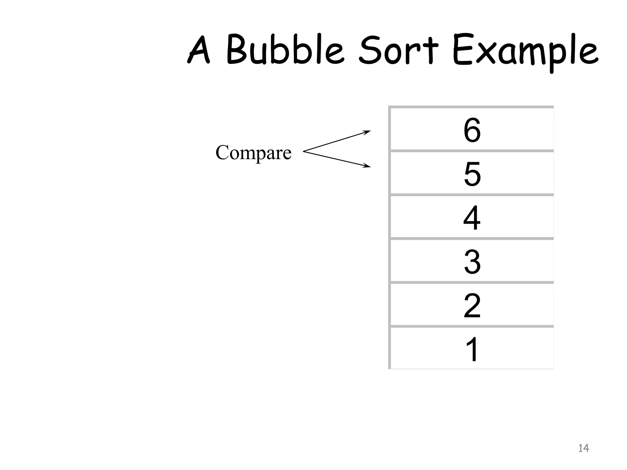
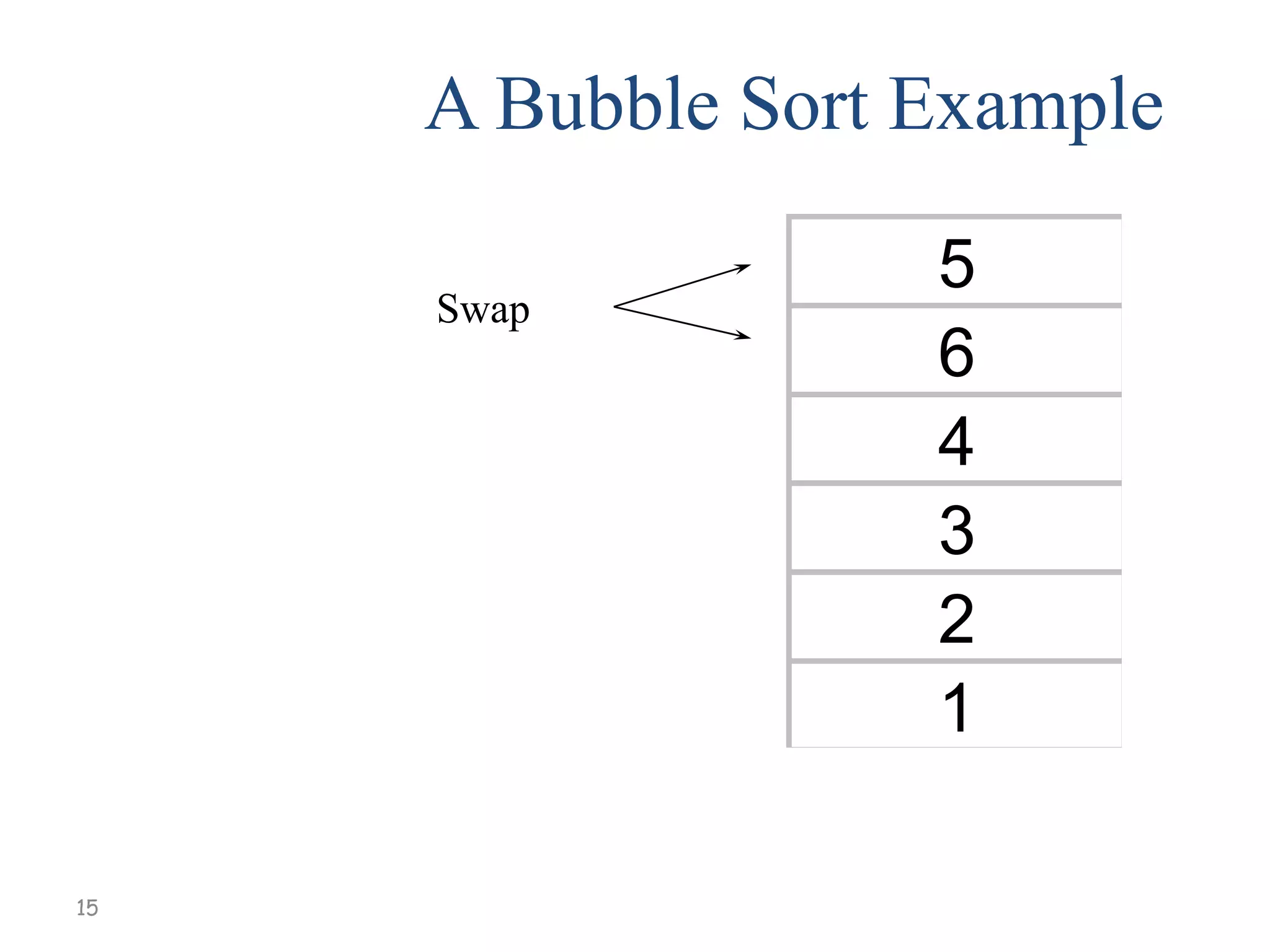
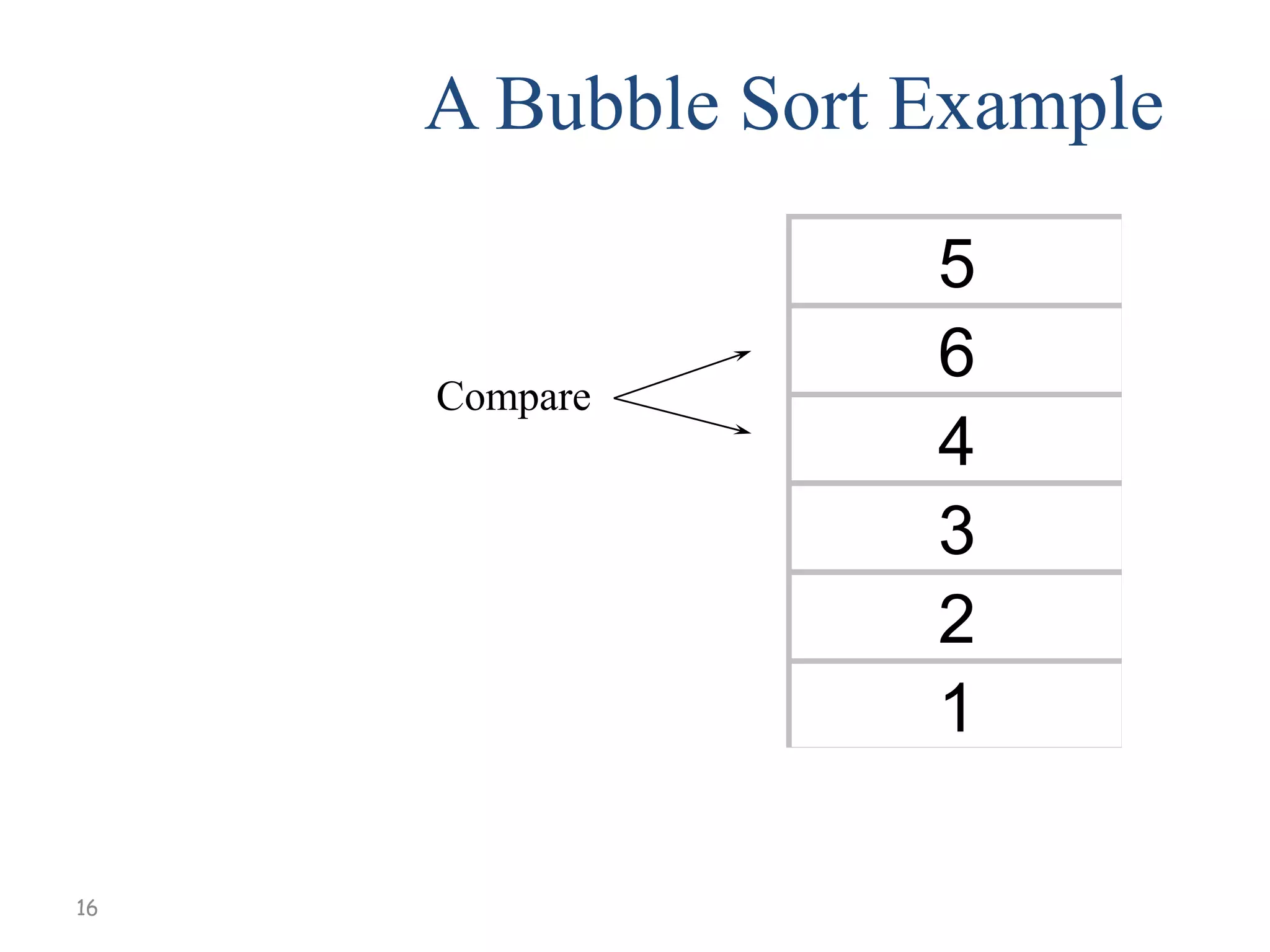
![Bubble Sort
Suppose the list of number A[1], [2], A[3], …,
A[N] is in memory. Algorithm works as
follows.
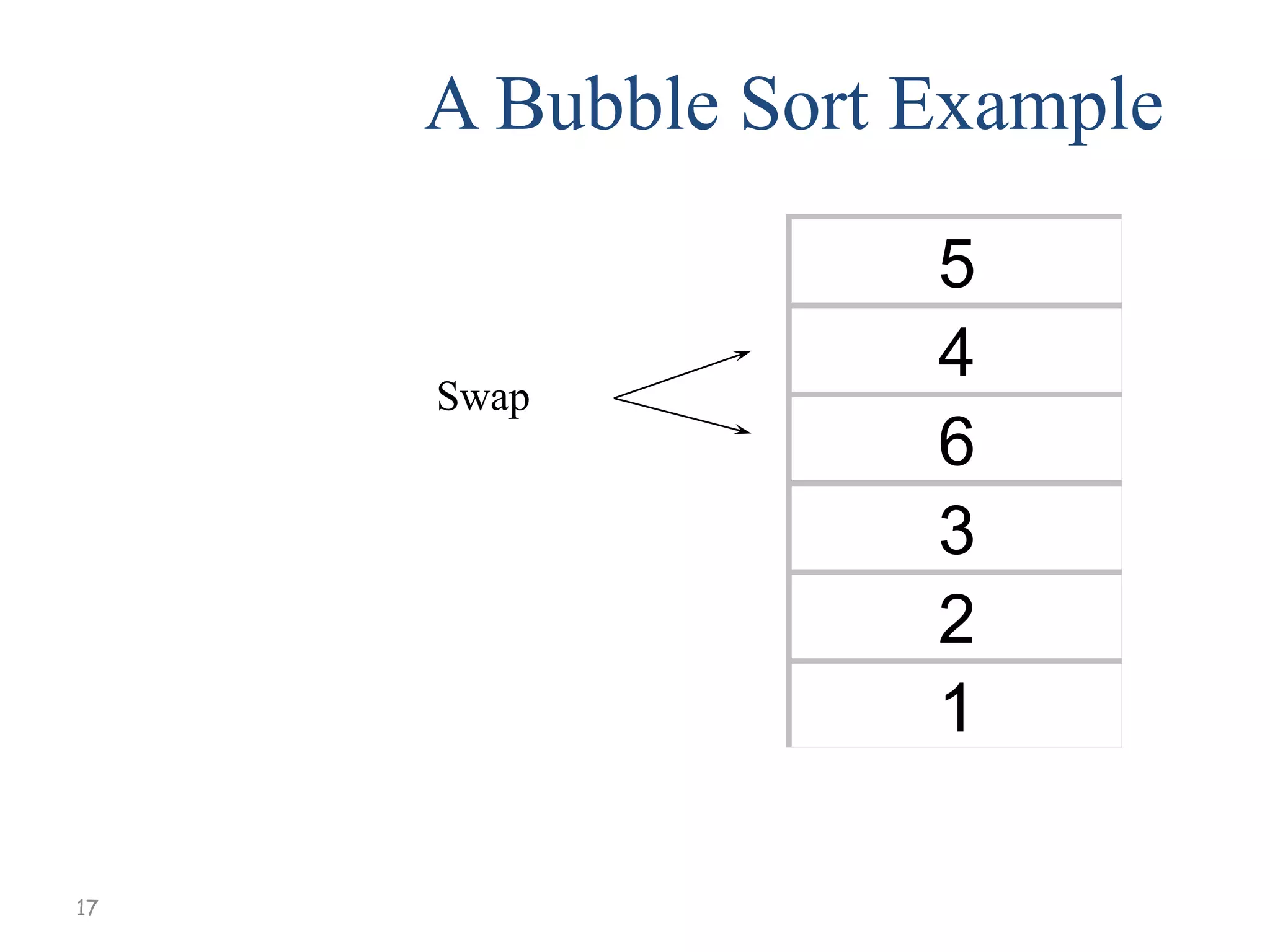
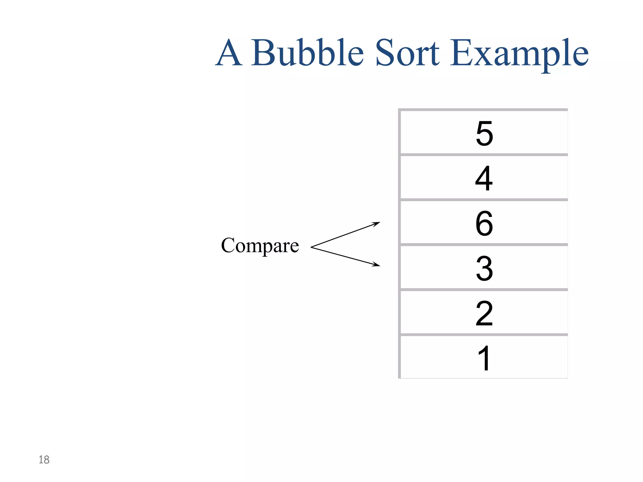
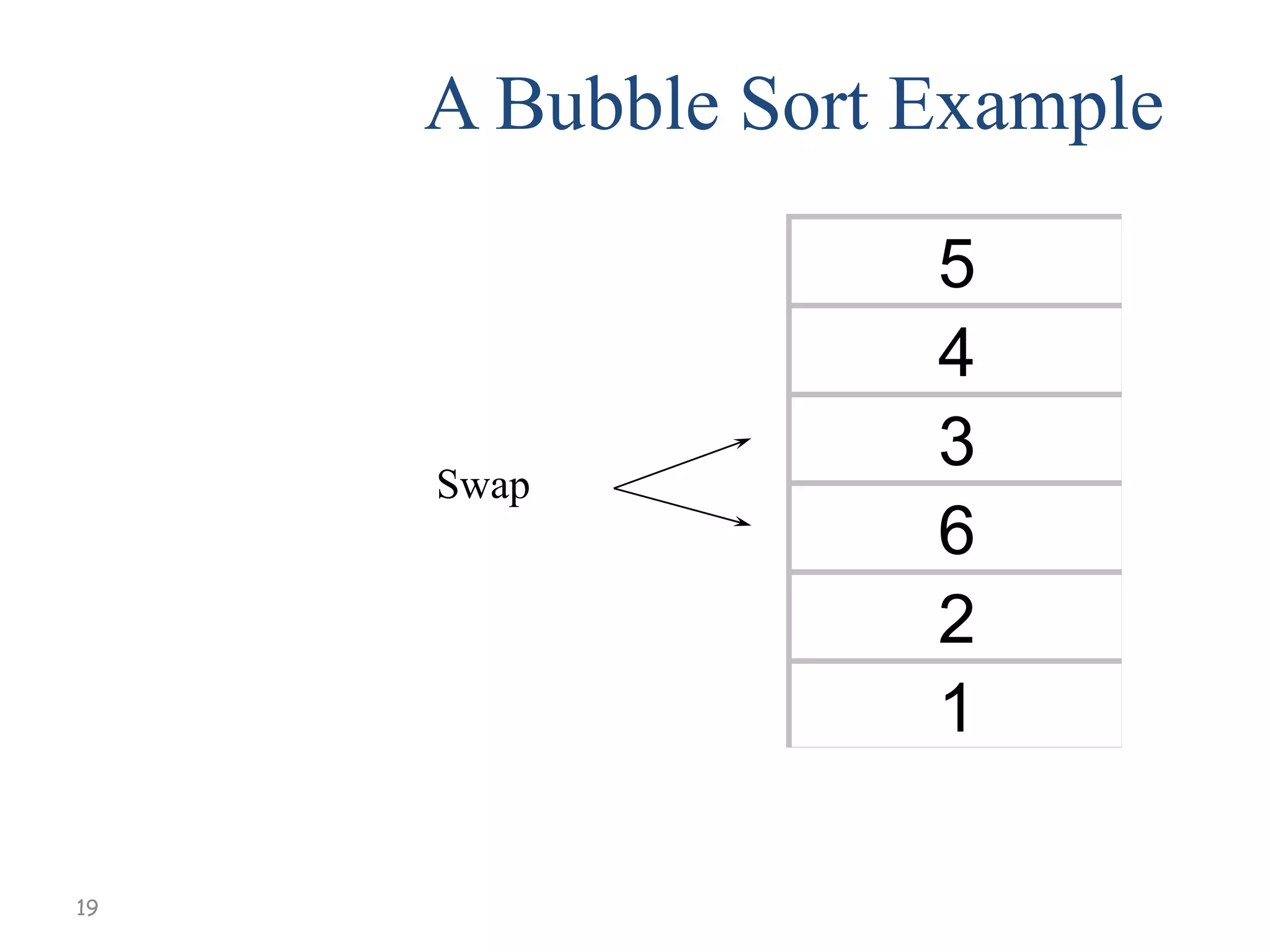
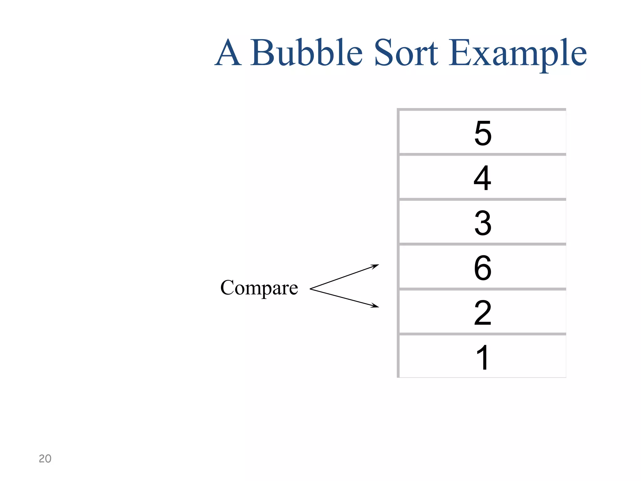
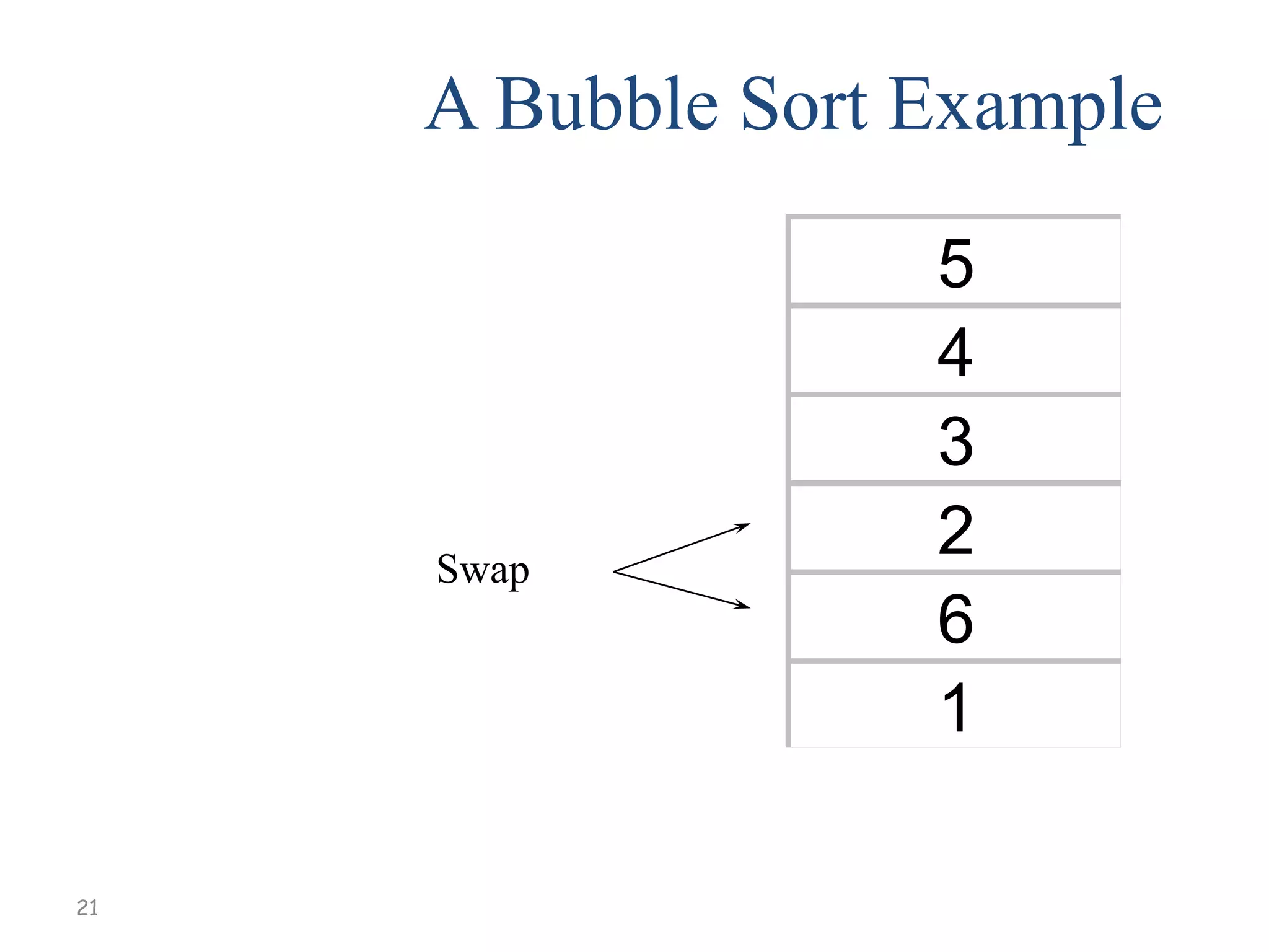
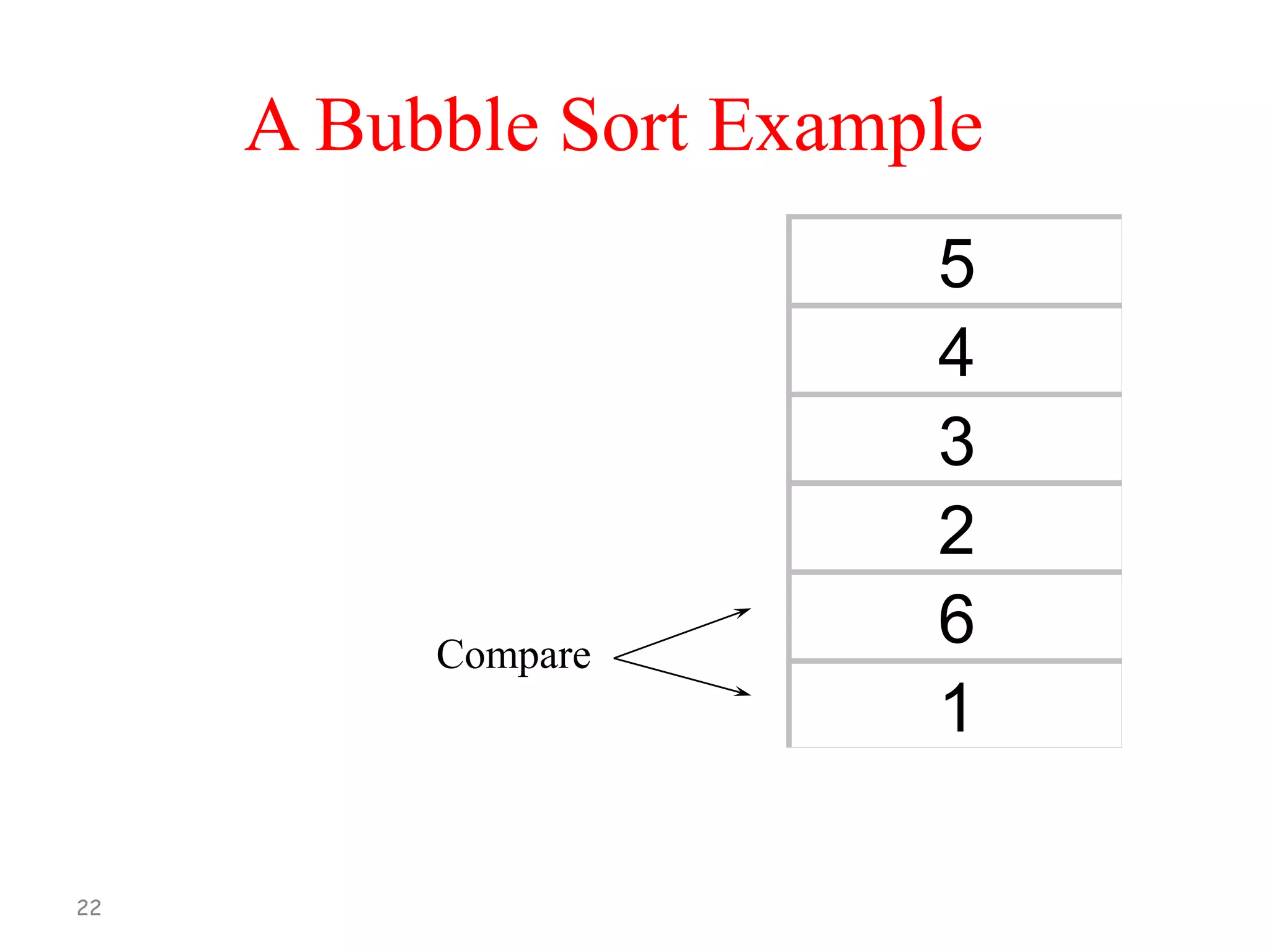
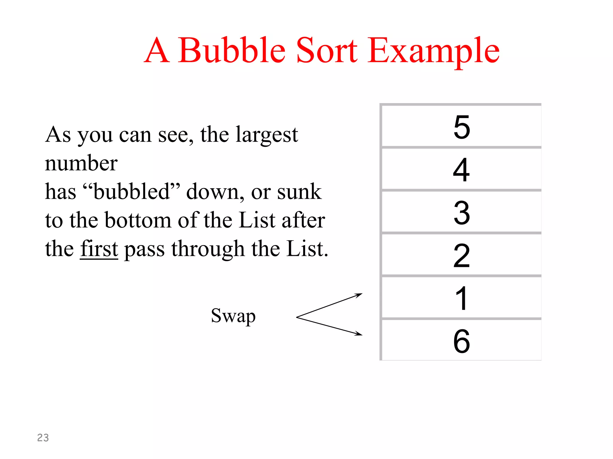
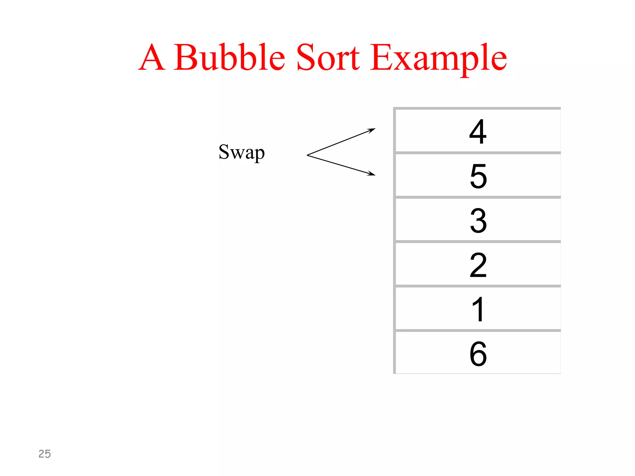
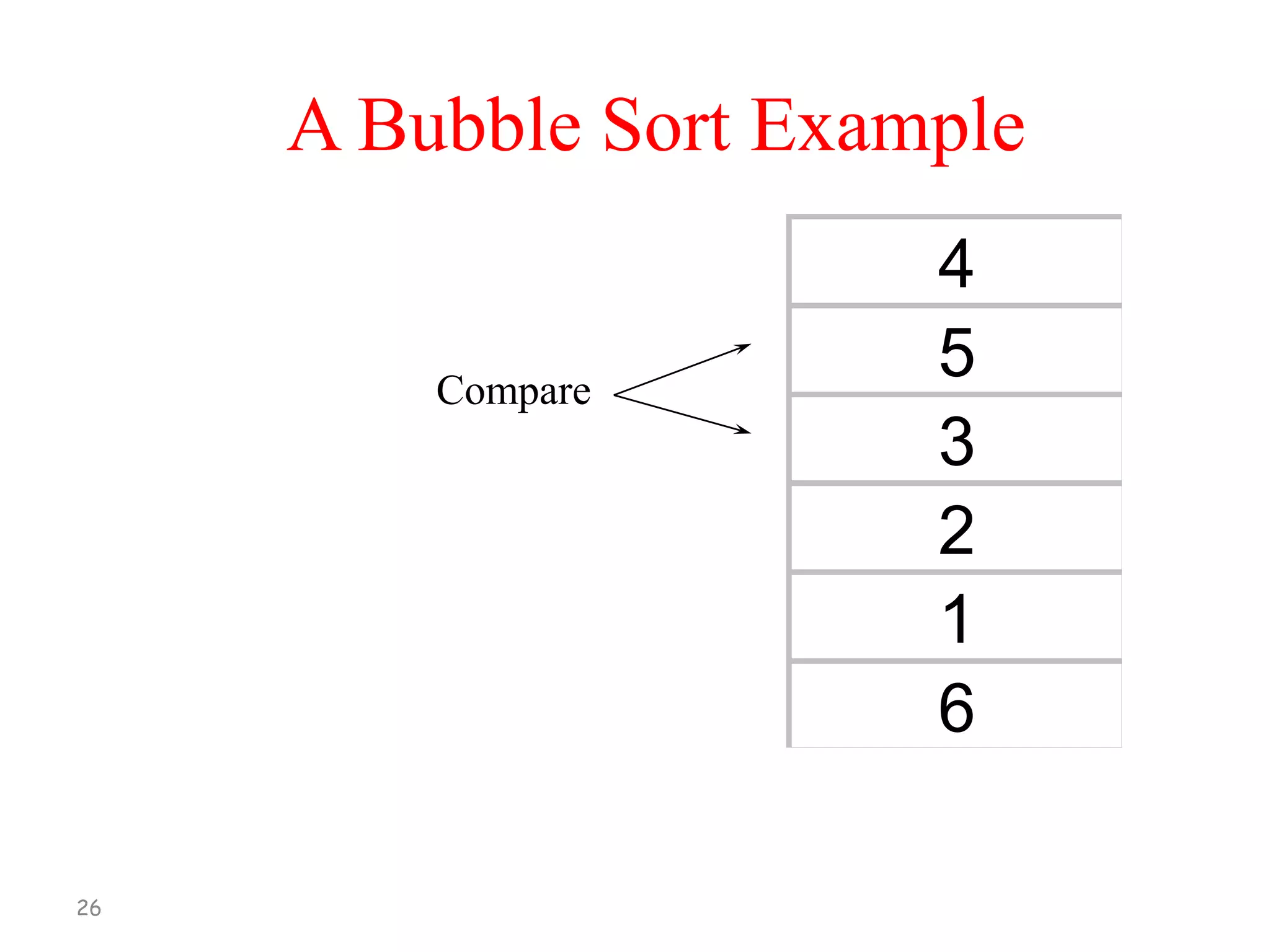
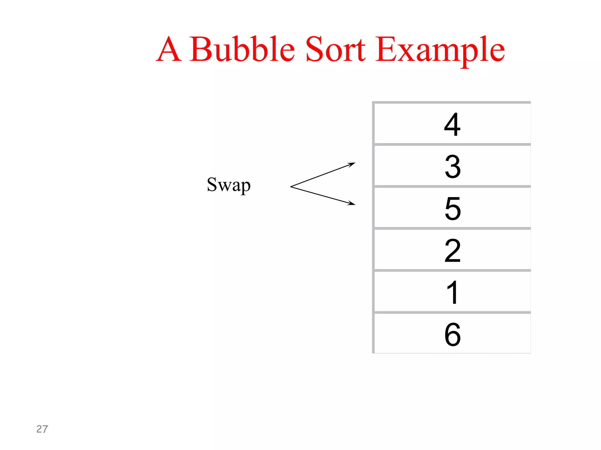
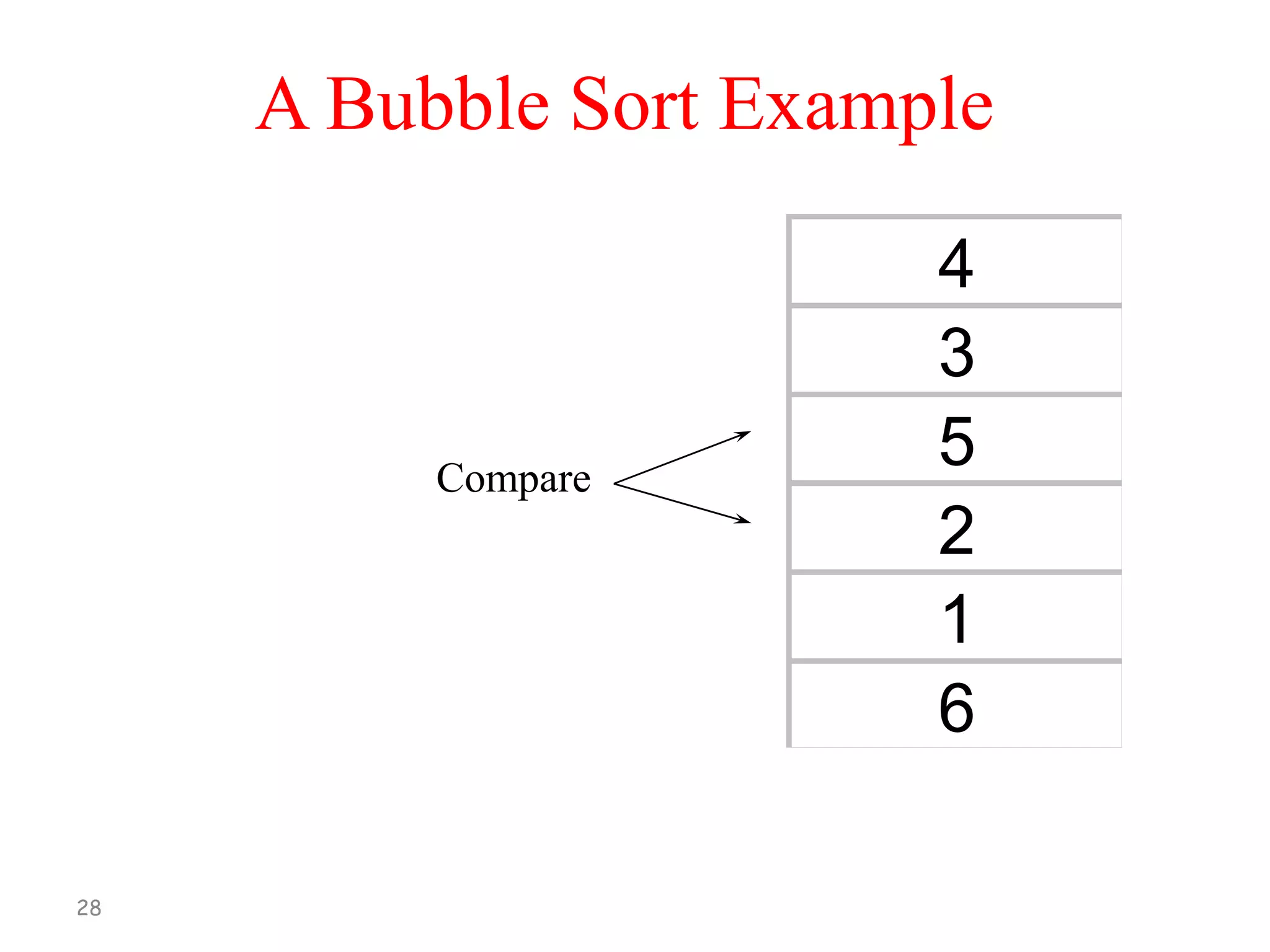
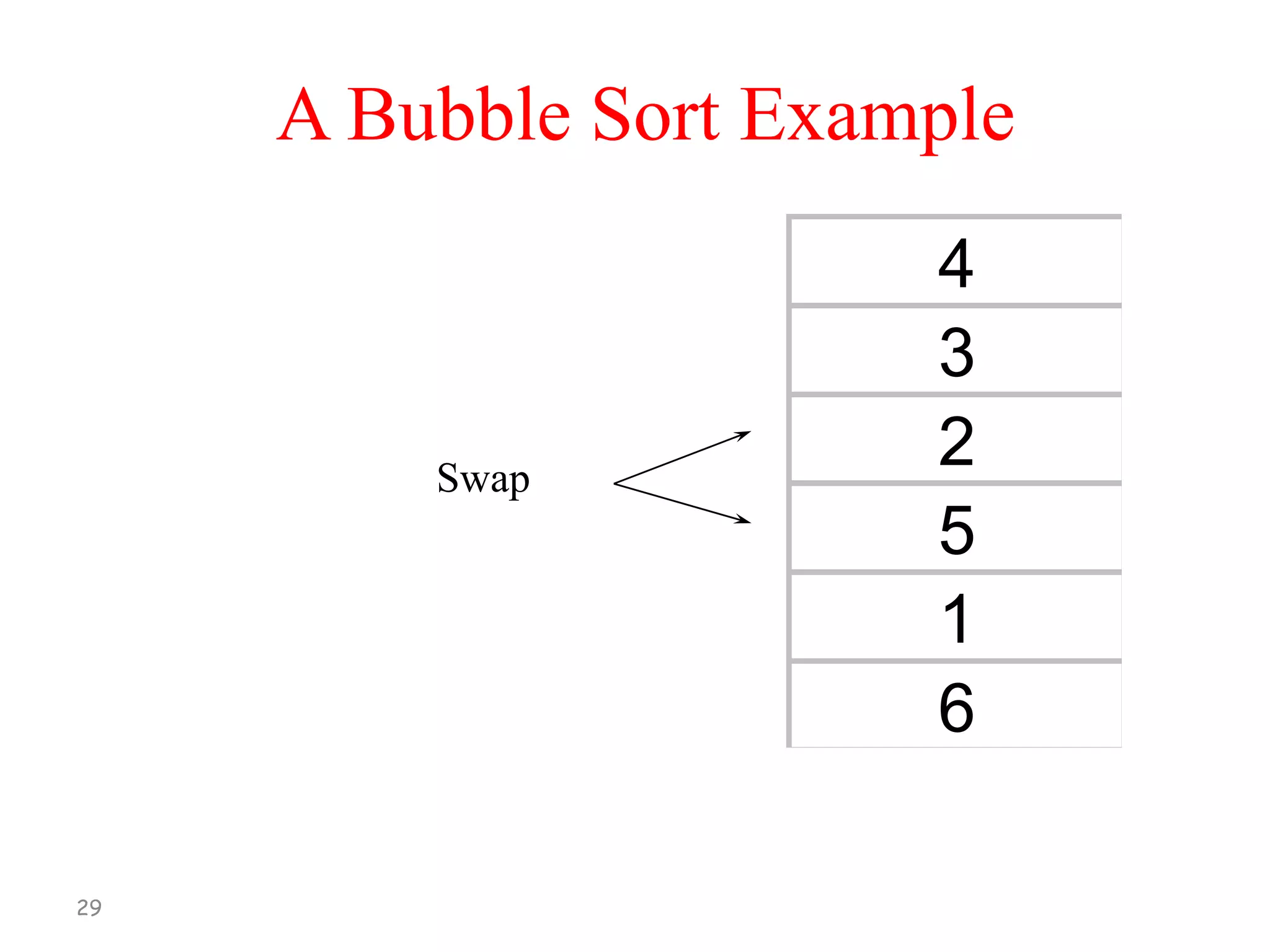
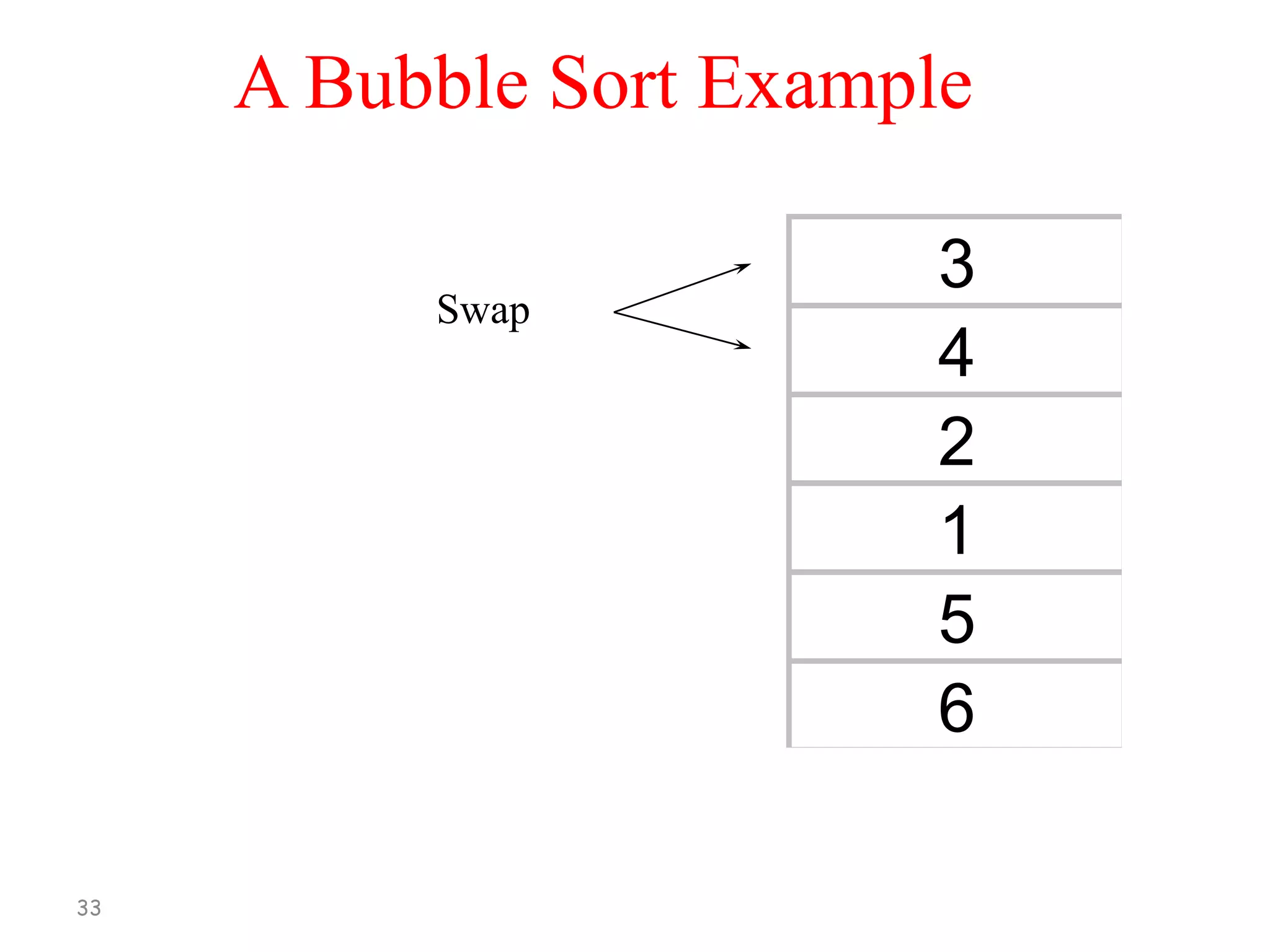
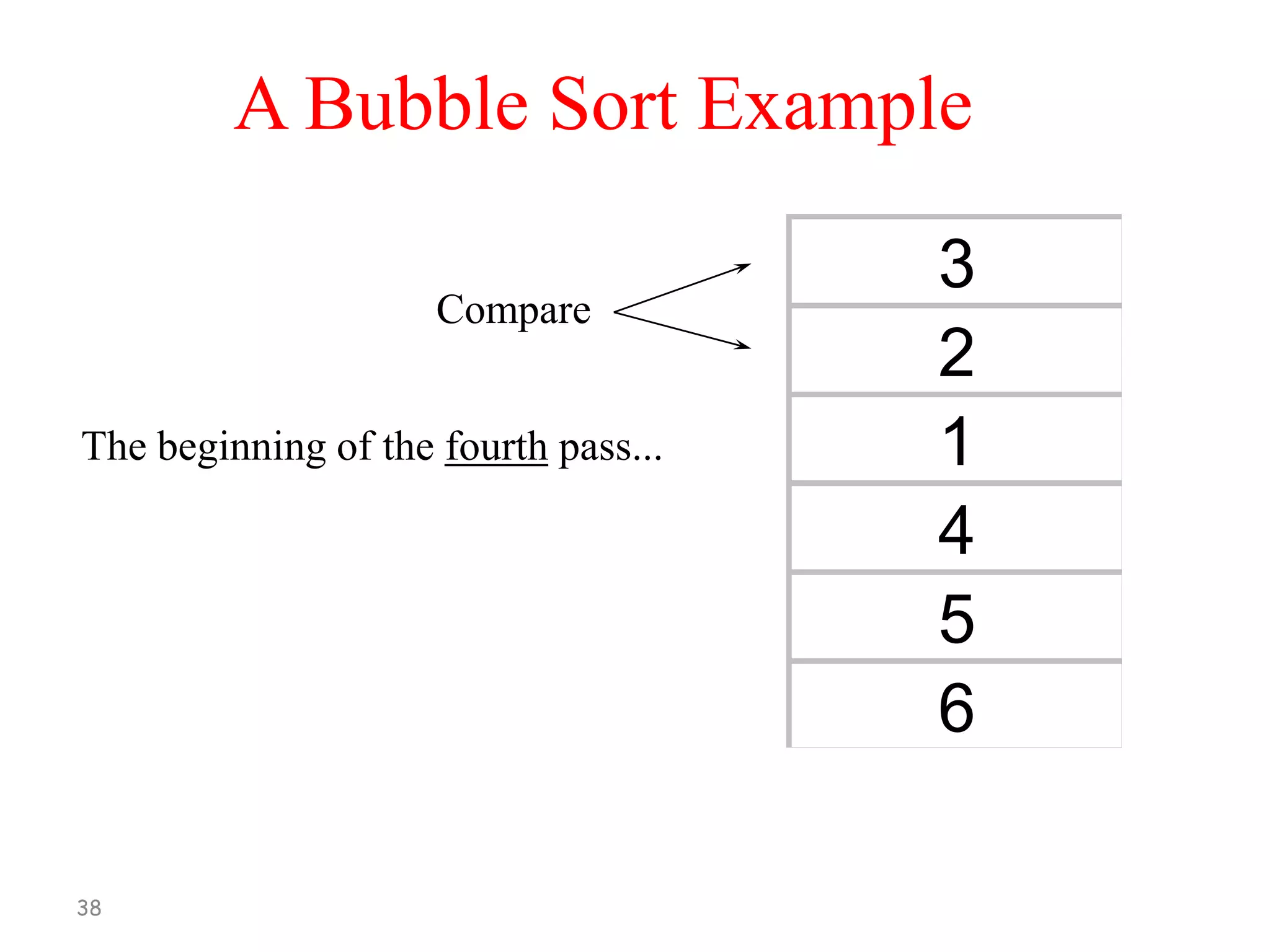
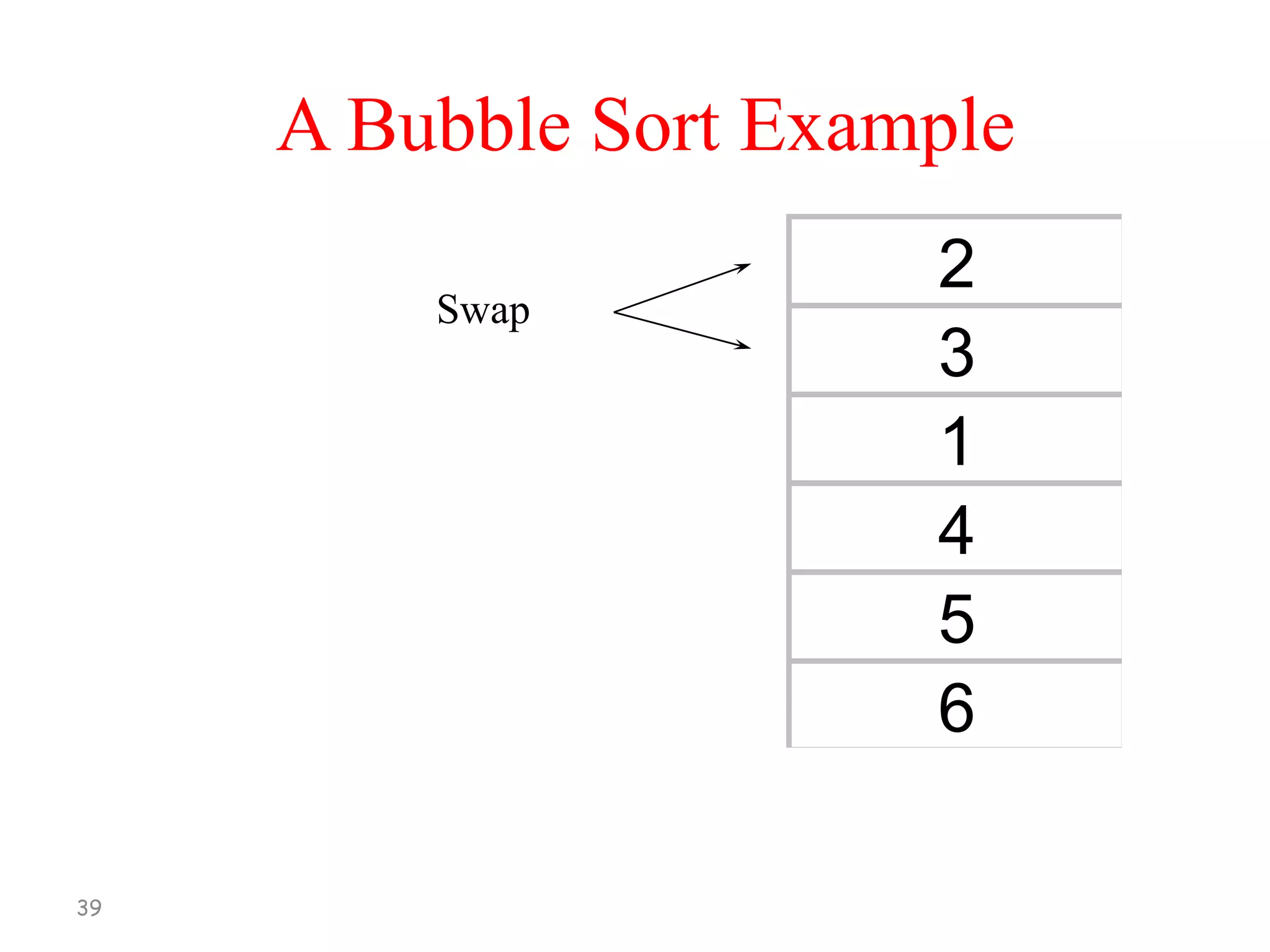
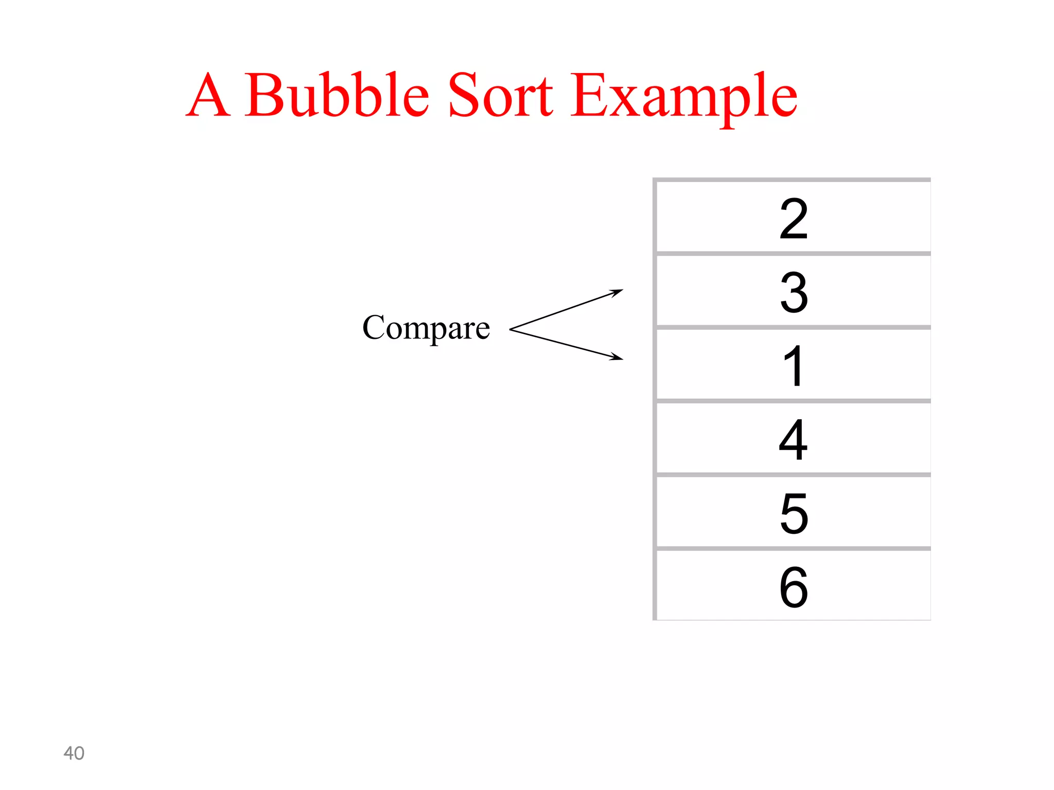
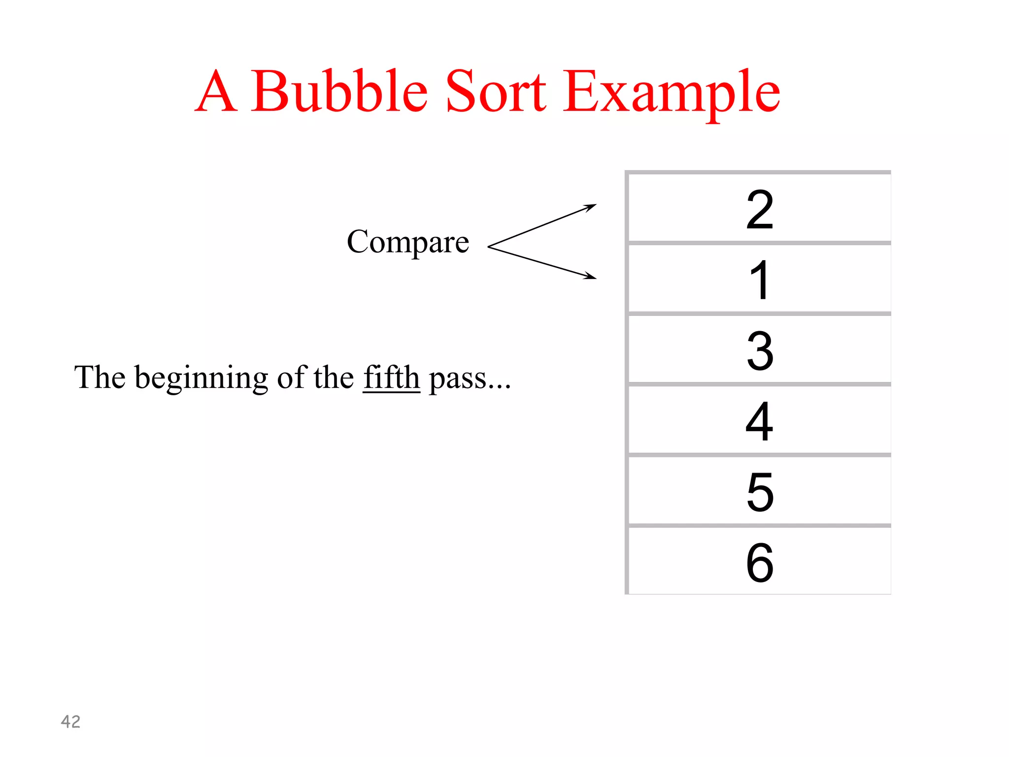
[1] Compare A[1] and A[2], arrange them in
the desired order so that A[1] < A[2]. Then
Compare A[2] and A[3], arrange them in
the desired order so that A[2] < A[3].
Continue until A[N-1] is compared with
A[N], arrange them so that A[N-1] < A[N].
12](https://image.slidesharecdn.com/lecture13-e-131122062304-phpapp01/75/Lecture-13-data-structures-and-algorithms-12-2048.jpg)
![Bubble Sort
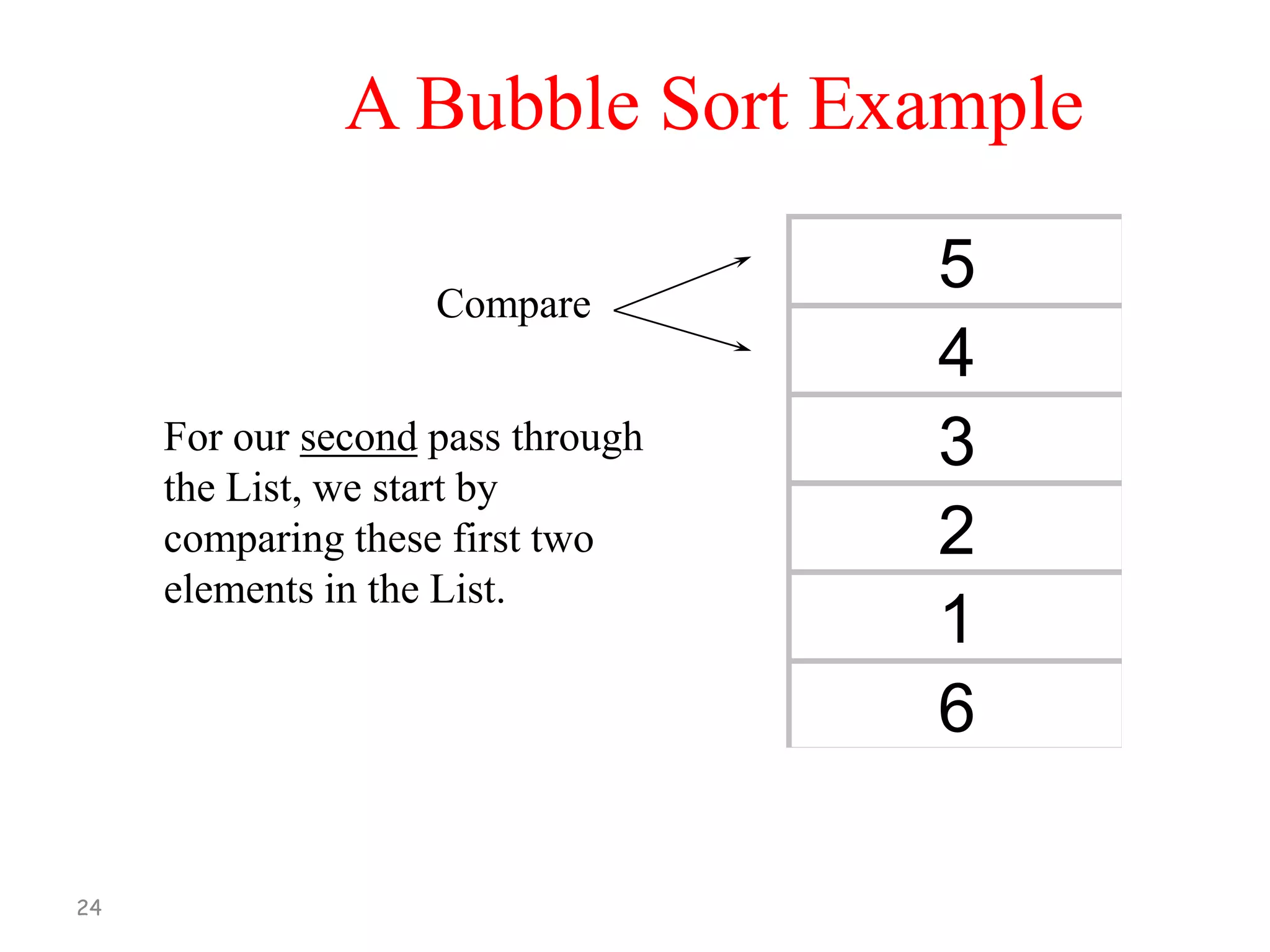
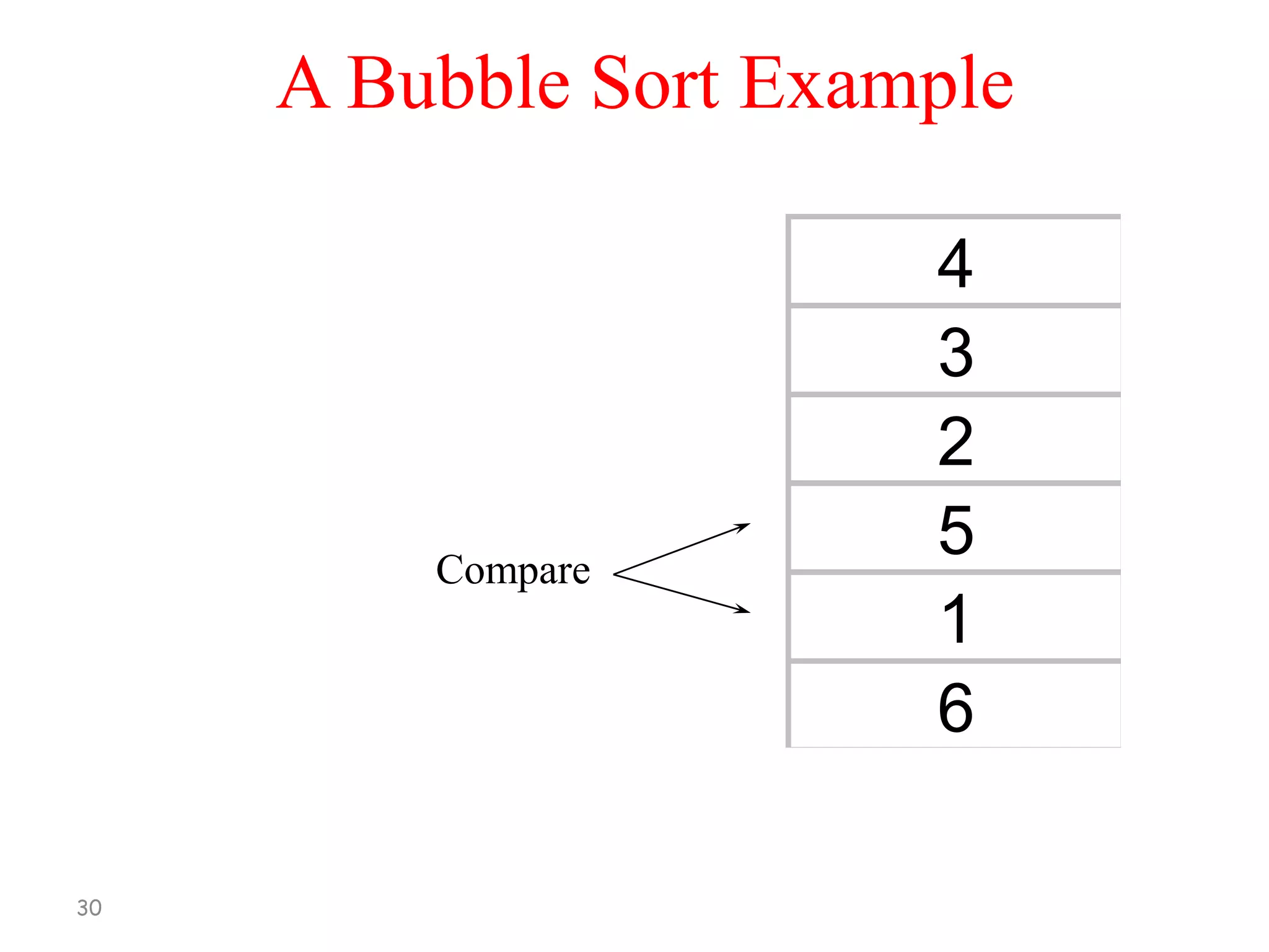
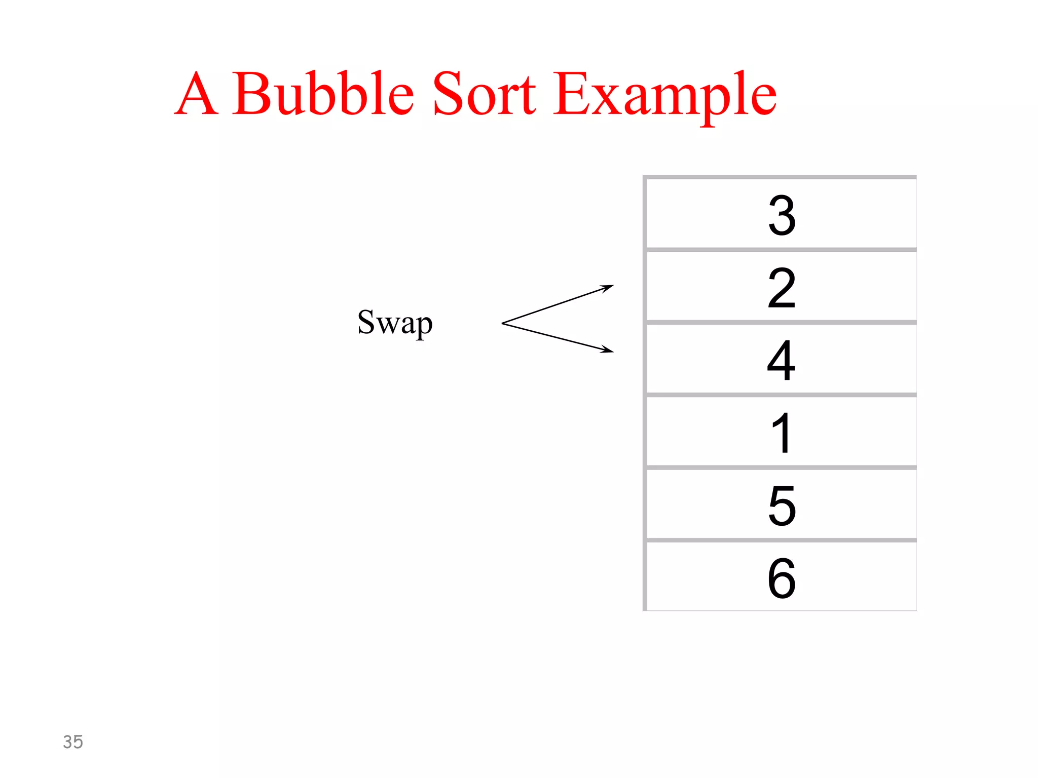
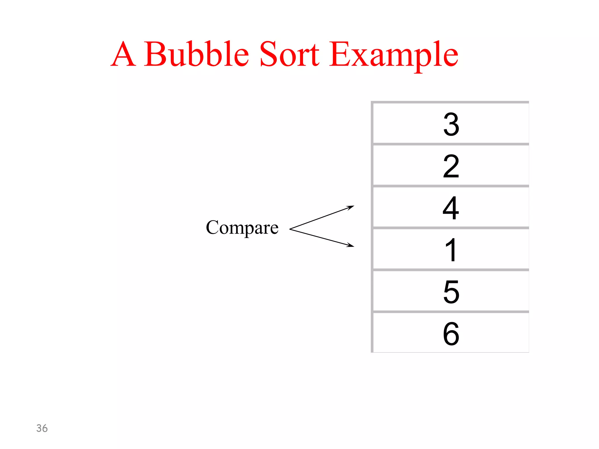
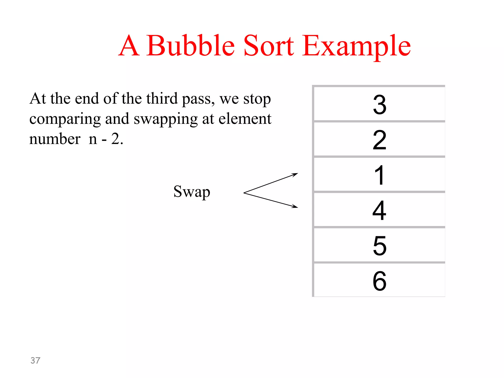
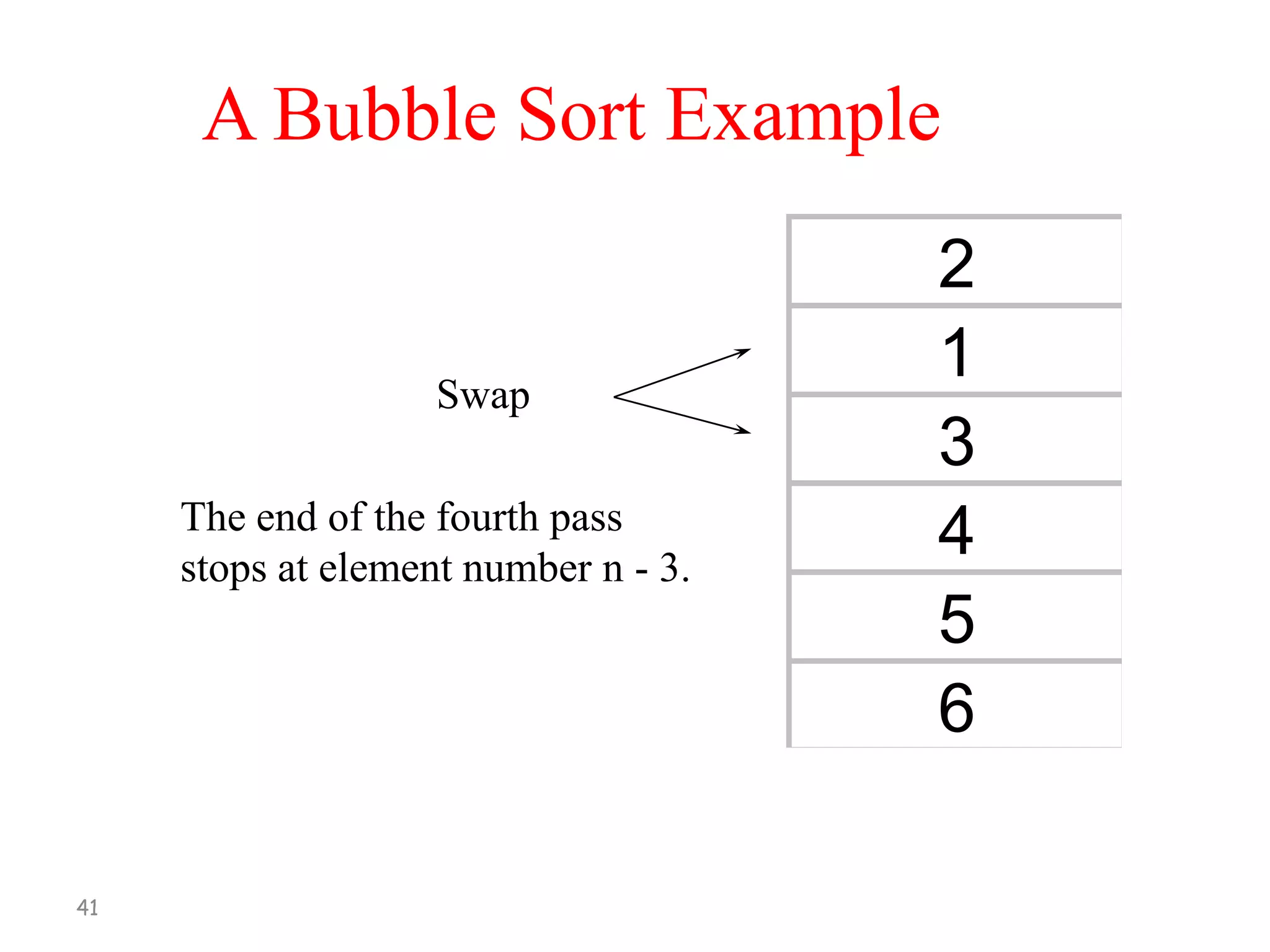
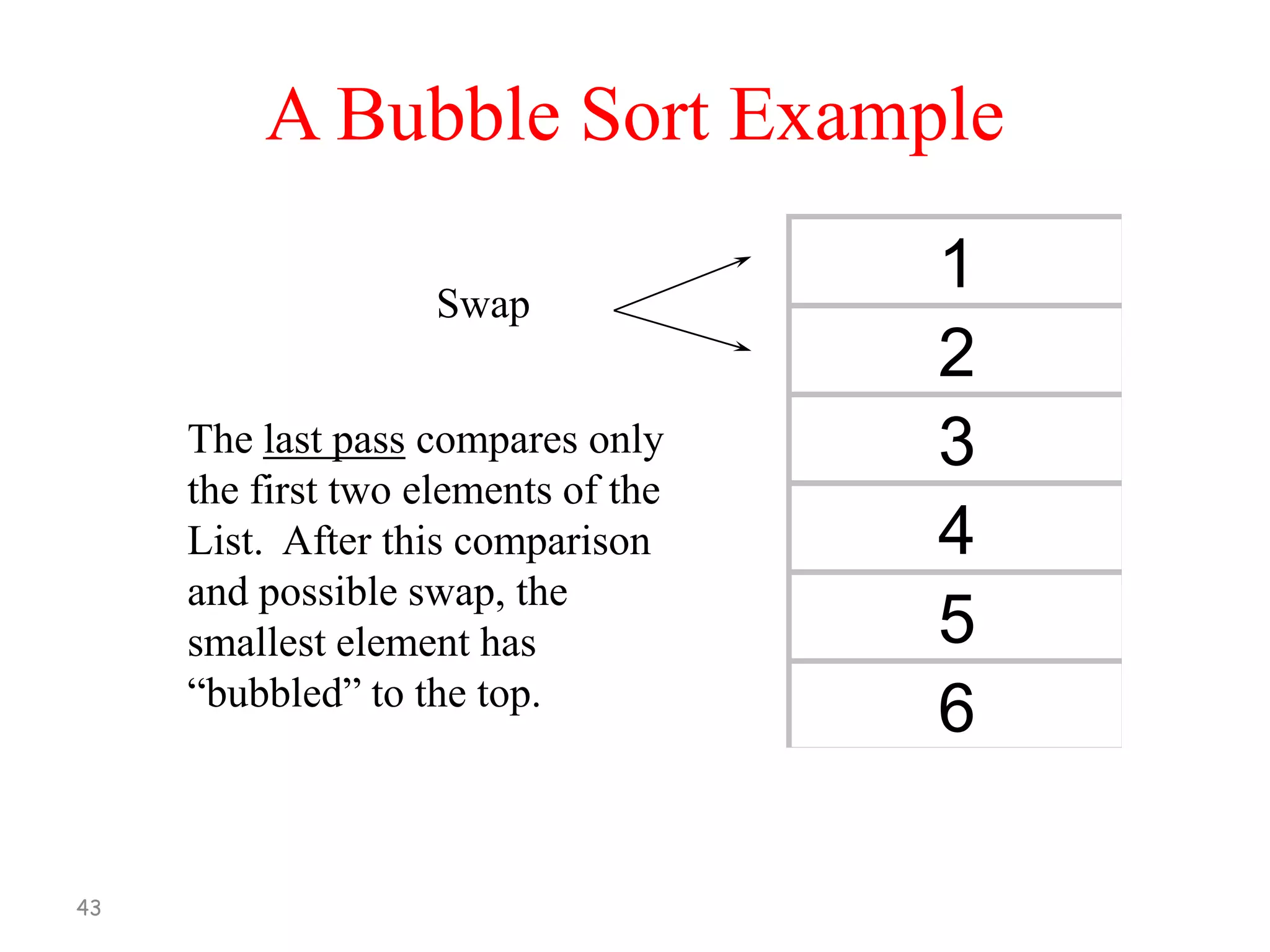
[2] Repeat Step 1, Now stop after comparing and
re-arranging A[N-2] and A[N-1].
[3] Repeat Step 3, Now stop after comparing and
re-arranging A[N-3] and A[N-2].
.
.
[N-1] Compare A[1] and A[2] and arrange them in
sorted order so that A[1] < A[2].
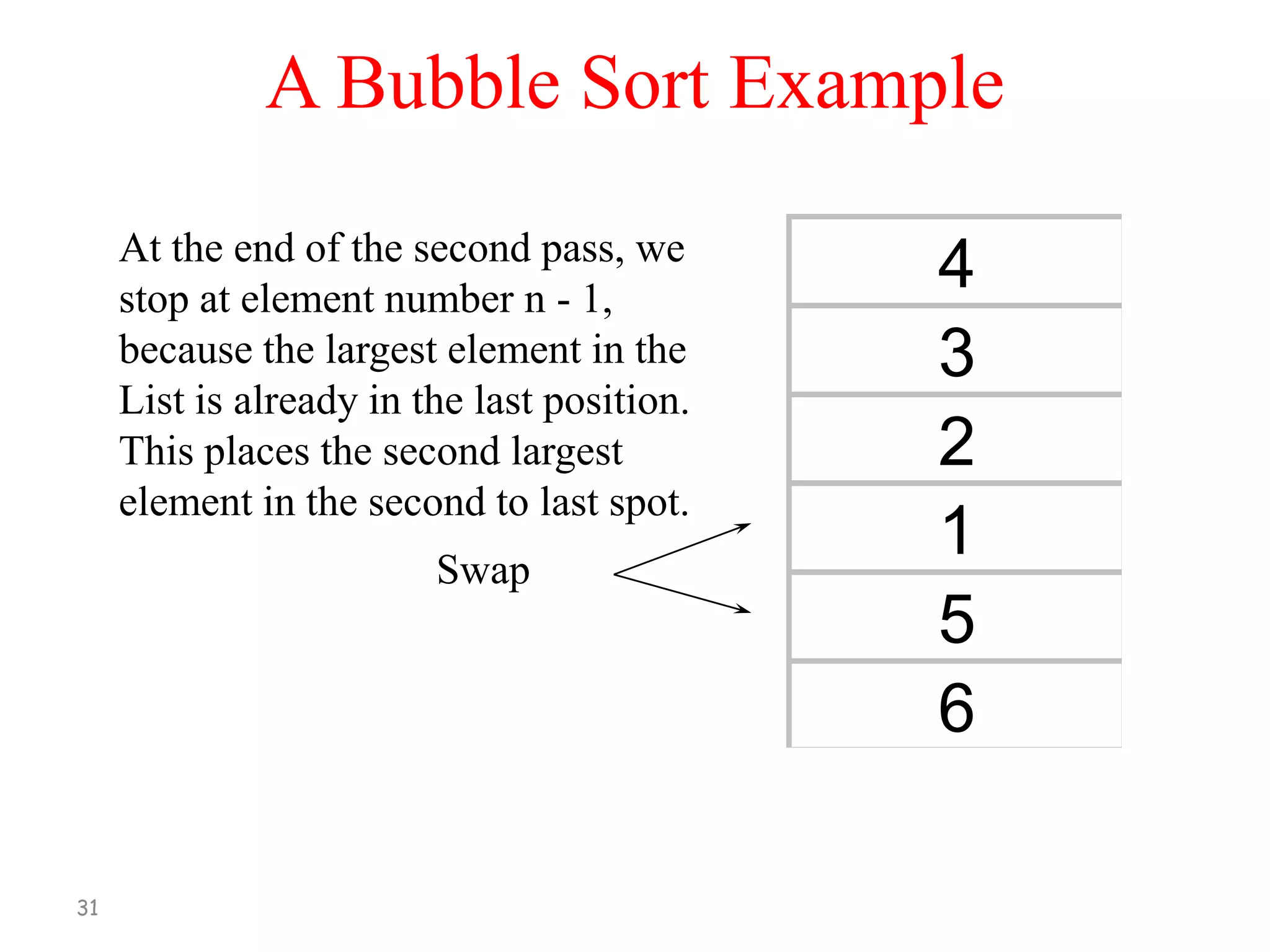
After N-1 steps the list will be sorted in
increasing order.
13](https://image.slidesharecdn.com/lecture13-e-131122062304-phpapp01/75/Lecture-13-data-structures-and-algorithms-13-2048.jpg)

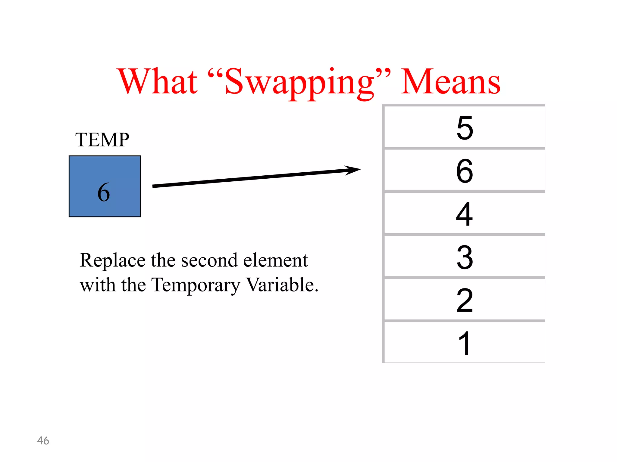
![Bubble Sort
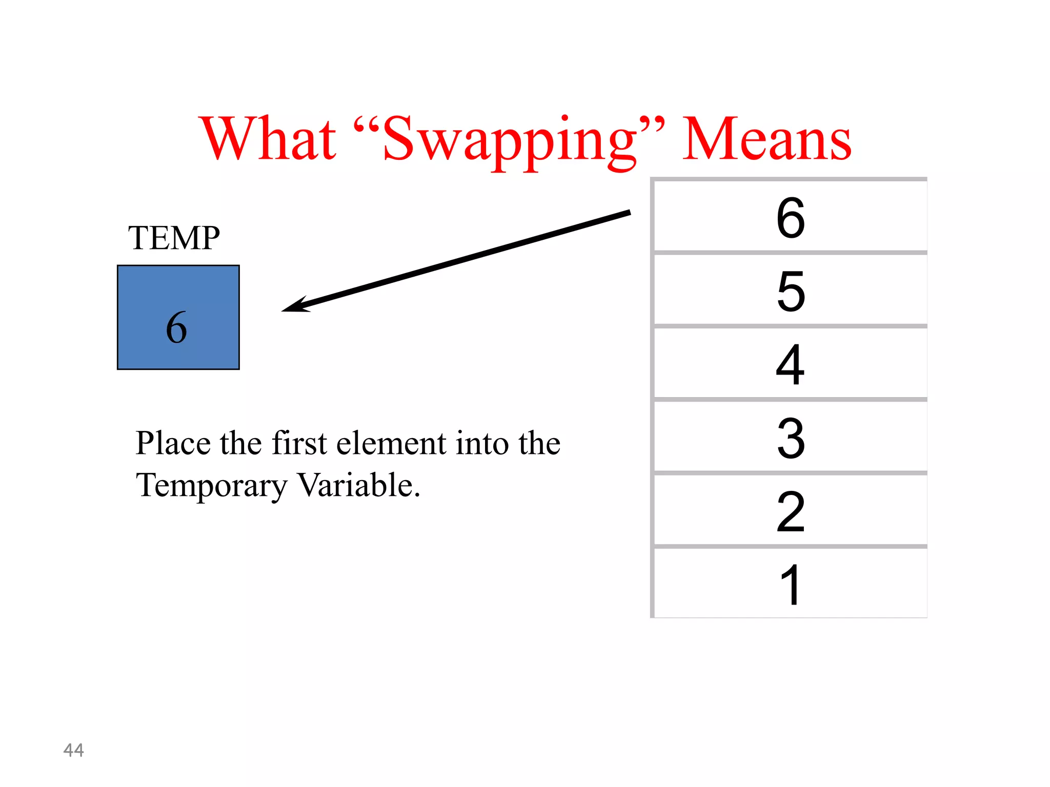
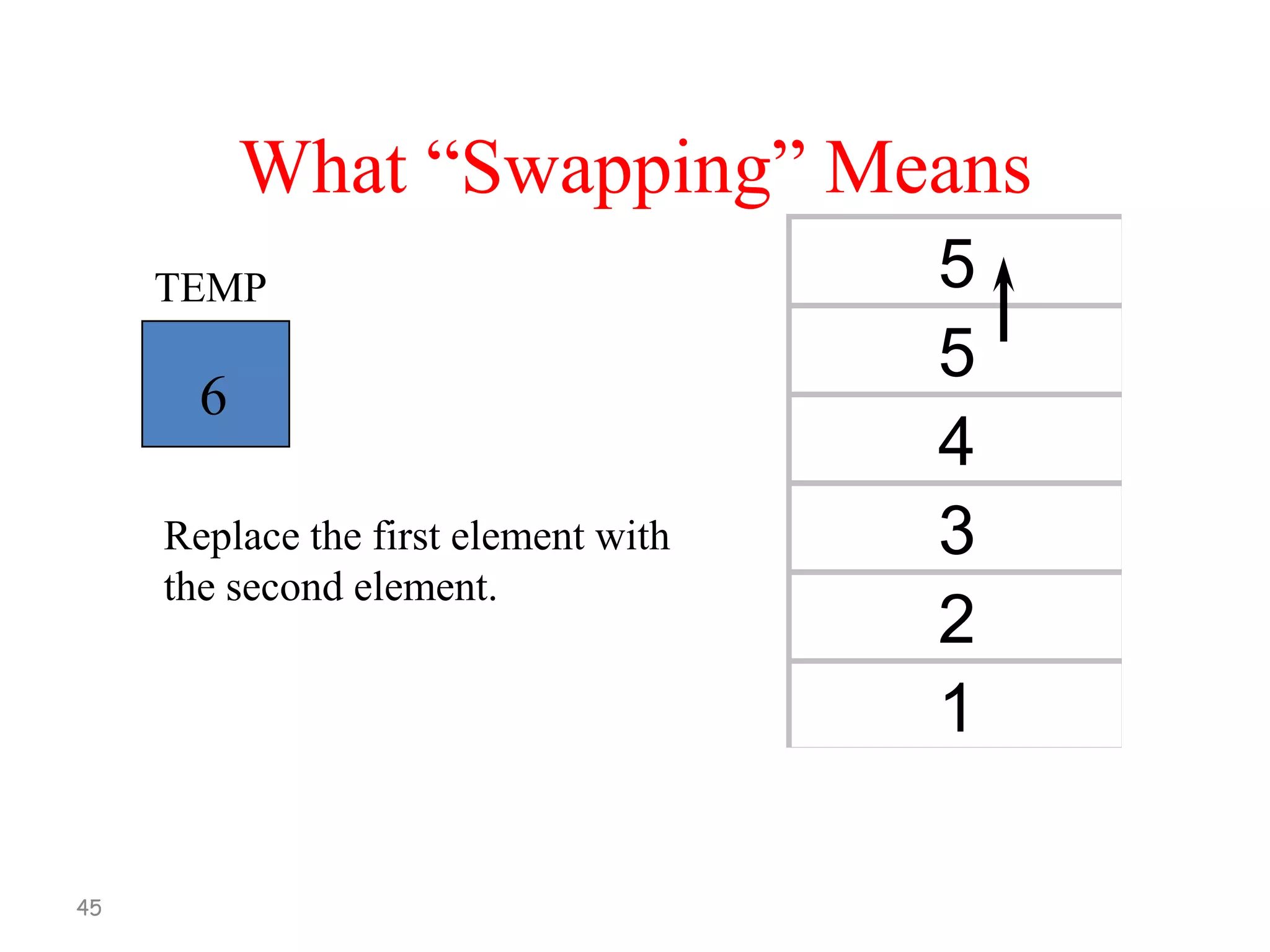
DATA is an array with N elements
[1] Repeat Step 2 and 3 for K =1 to N-1
[2] Set PTR :=1
[3] Repeat While PTR <= N –K
(a) If DATA[PTR] > DATA[PTR+1]
Interchange DATA[PTR] and
DATA[PTR + 1]
(b) Set PTR = PTR + 1
[4] Exit
47](https://image.slidesharecdn.com/lecture13-e-131122062304-phpapp01/75/Lecture-13-data-structures-and-algorithms-47-2048.jpg)
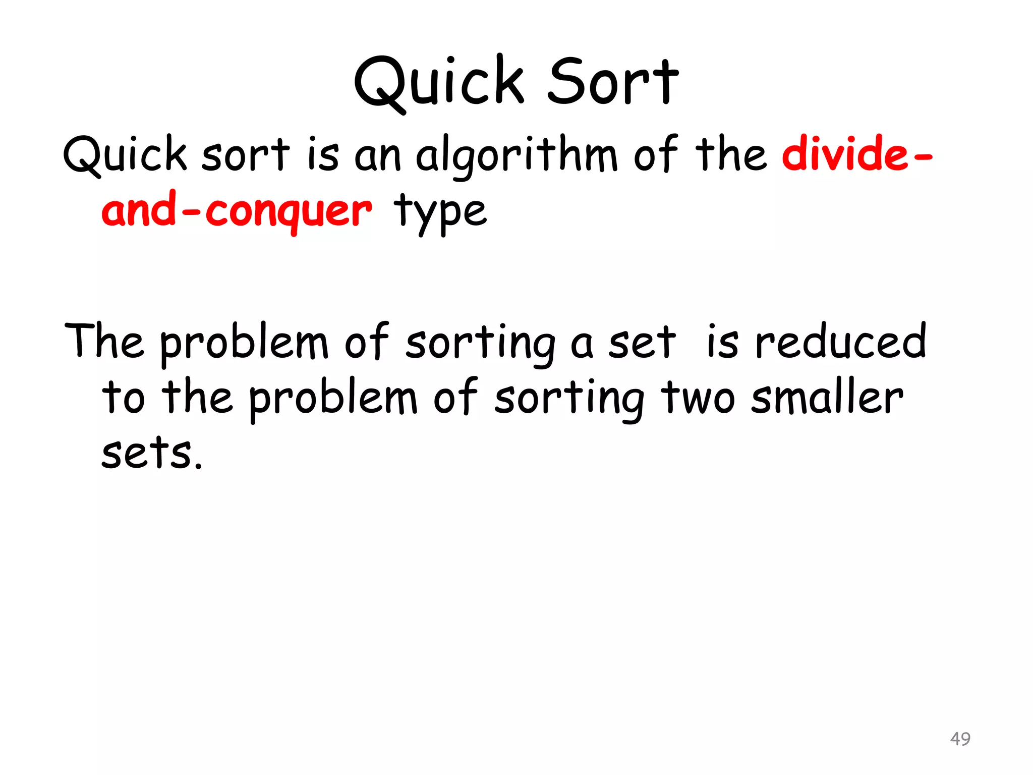
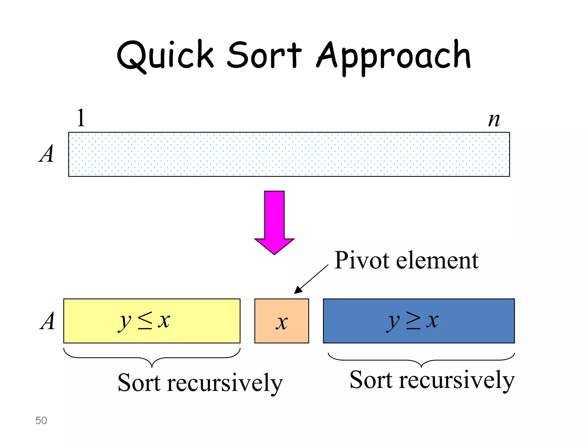
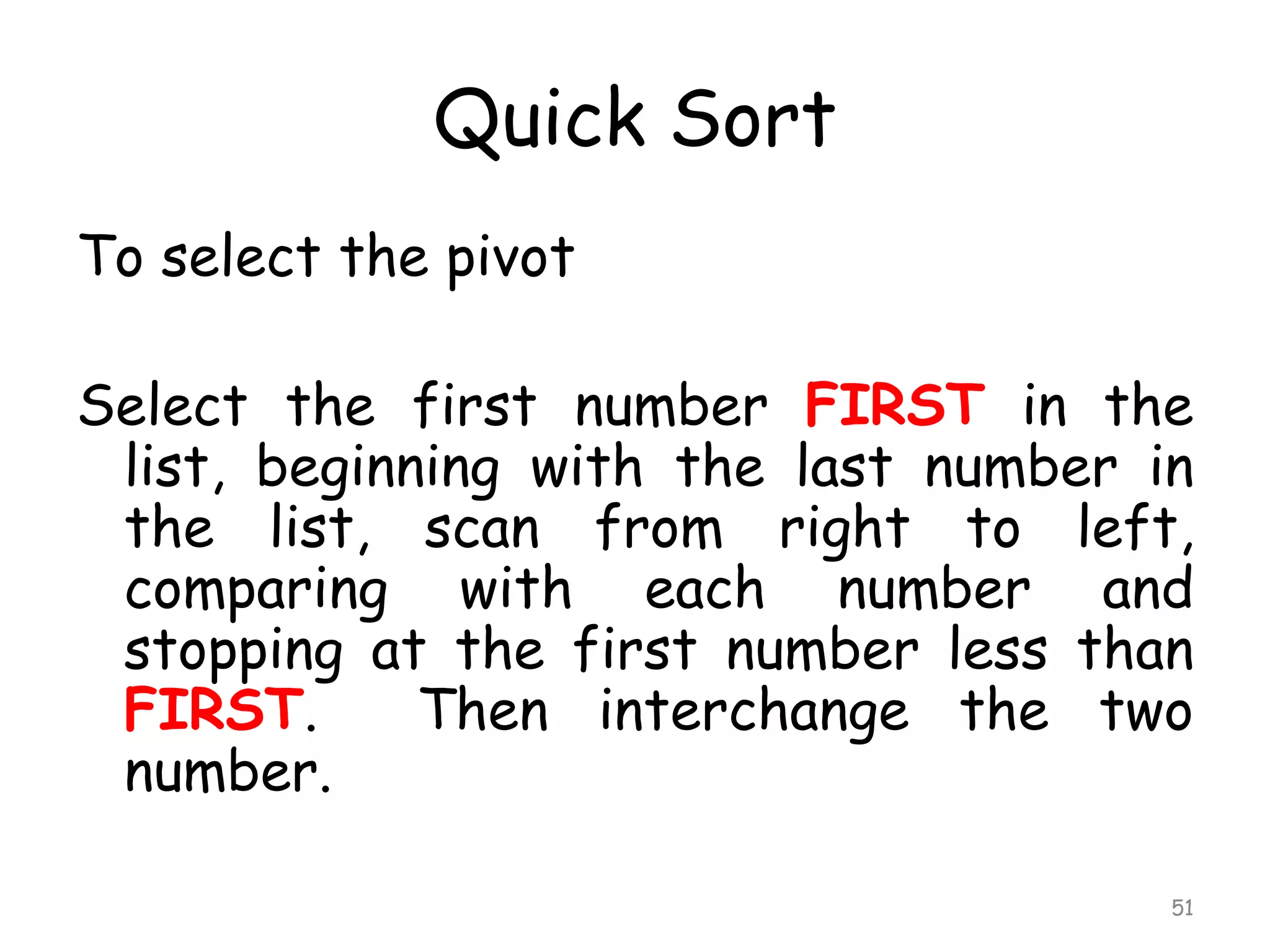
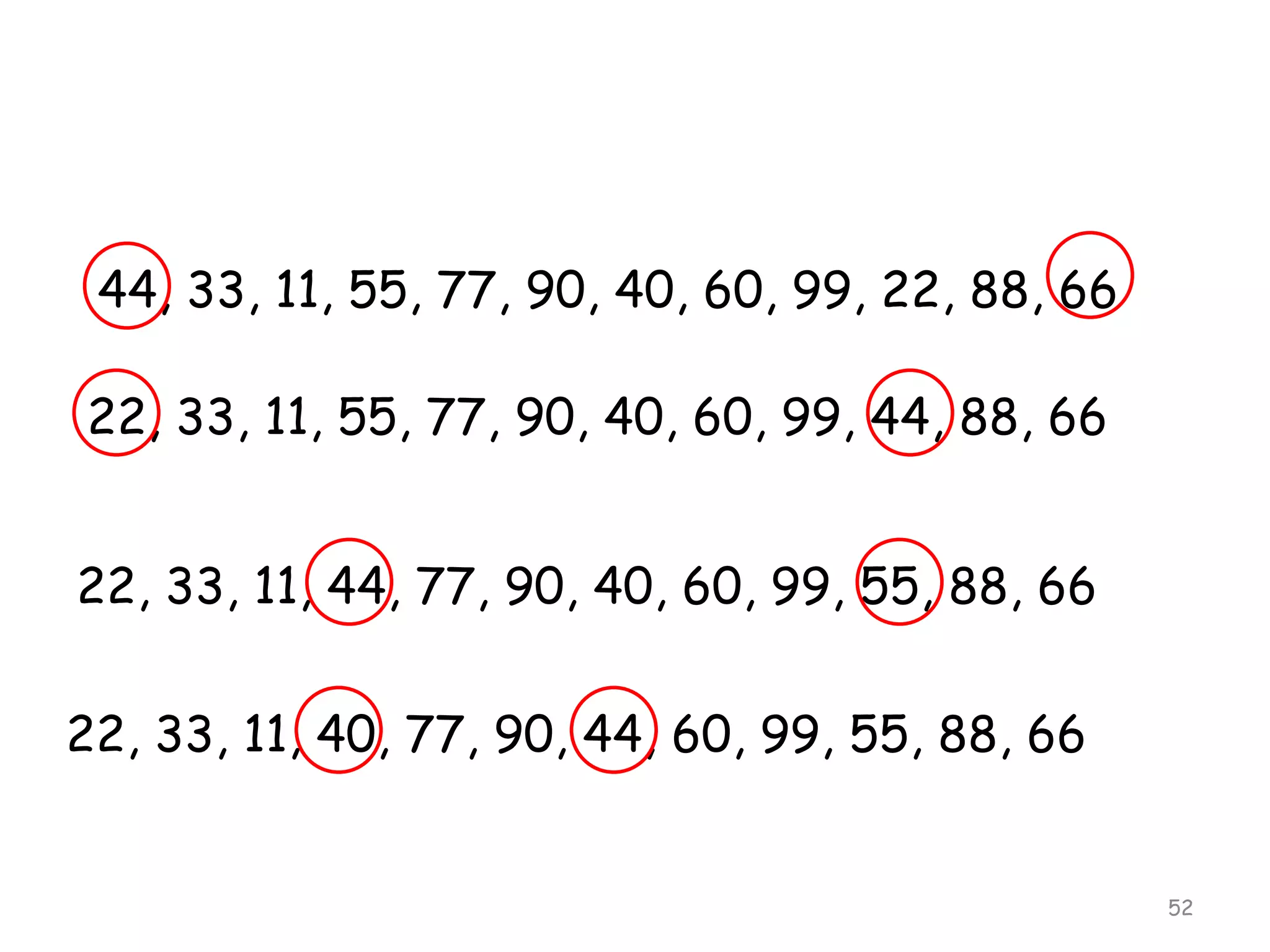
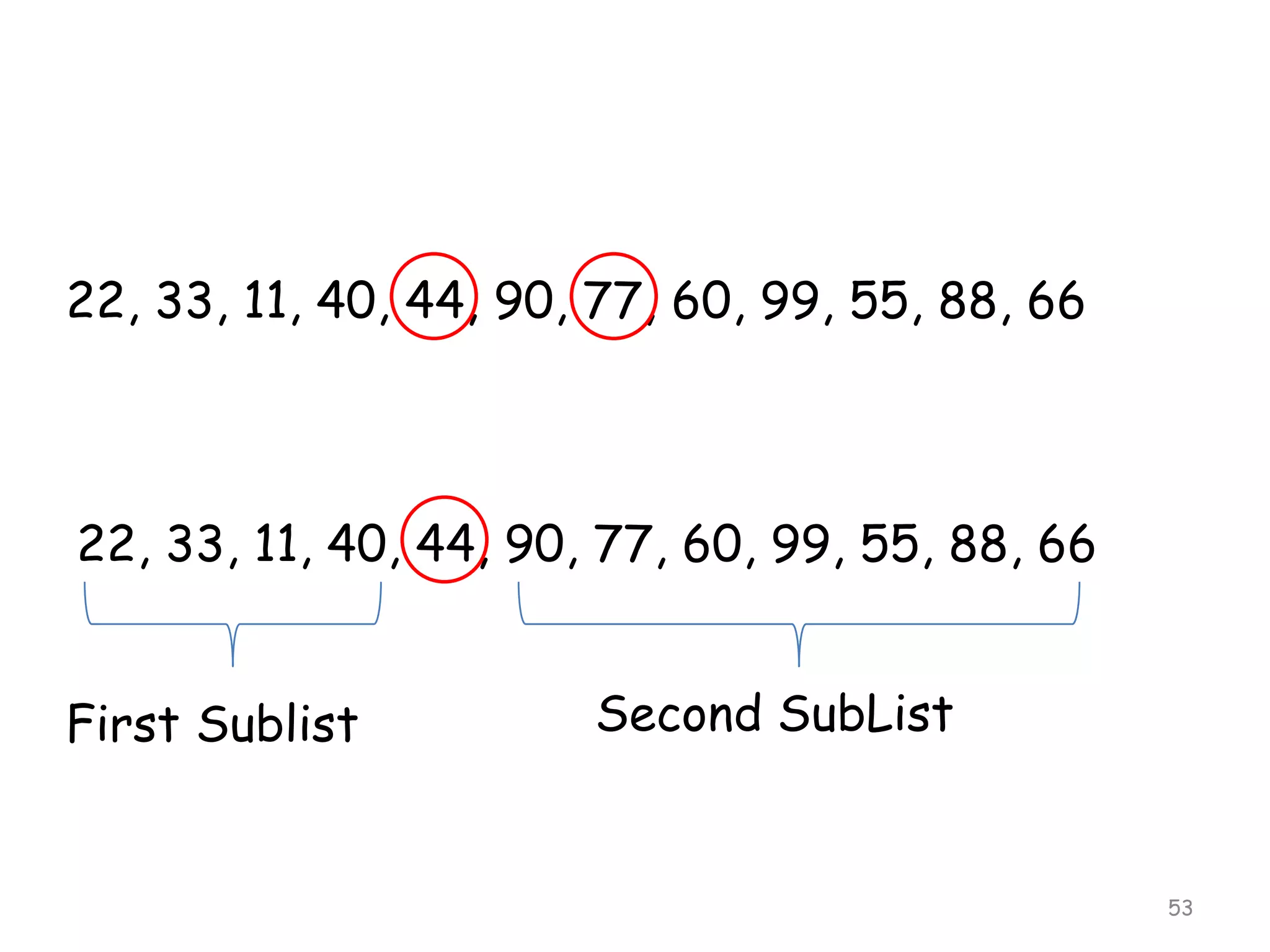
![Quick Sort Algorithm
Input: Unsorted sub-array A[first..last]
Output: Sorted sub-array A[first..last]
QUICKSORT (A, first, Last)
if first < last
then loc← PARTITION(A, first, last)
QUICKSORT (A, first, loc-1)
QUICKSORT (A, loc+1, last)
54](https://image.slidesharecdn.com/lecture13-e-131122062304-phpapp01/75/Lecture-13-data-structures-and-algorithms-54-2048.jpg)
![Partition Algorithm
Input: Sub-array A[first..last]
Output: Sub-array A[first..loc] where each element of
A[first..loc-1] is ≤ to each element of A[(q+1)..r]; returns the
index loc
PARTITION (A, first, last)
1
2
3
4
5
6
7
8
9
10
11
55
x ← A[first]
i ← first -1
j ← last +1
while TRUE
repeat j ← j - 1
until A[j] ≤ x
repeat i ← i + 1
until A[i] ≥ x
if i < j
then exchange A[i] ↔A[j]
else return j](https://image.slidesharecdn.com/lecture13-e-131122062304-phpapp01/75/Lecture-13-data-structures-and-algorithms-55-2048.jpg)
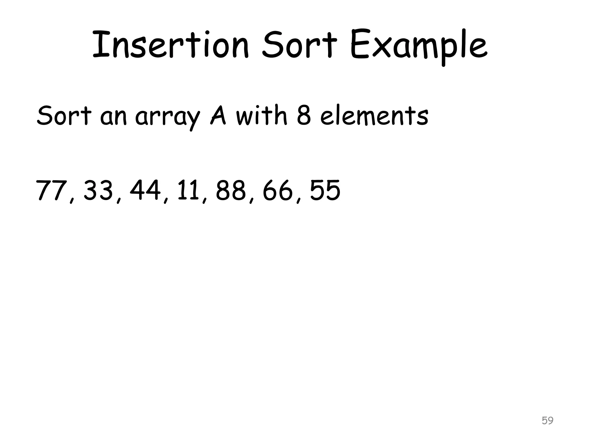
![Insertion Sort
An array A with N elements A[1], A[2] …
A[N] is in memory
Insertion Sort scan A from A[1] to A[N]
inserting each elements A[k] into its
proper position in the previously sorted
subarray A[1], A[2], …. A[K-1]
56](https://image.slidesharecdn.com/lecture13-e-131122062304-phpapp01/75/Lecture-13-data-structures-and-algorithms-56-2048.jpg)
![Pass 1: A[1] by itself is trivially sorted
Pass 2: A[2] is inserted either before or
after A[1] so that A[1], A[2] is sorted
Pass 3: A[3] is inserted in its proper place
in A[1], A[2], that is before A[1],
between A[1] and A[2] or after A[2] so
that A[1], A[2], A[3] is sorted.
57](https://image.slidesharecdn.com/lecture13-e-131122062304-phpapp01/75/Lecture-13-data-structures-and-algorithms-57-2048.jpg)
![Pass 4: A[4] is inserted in its proper place in
A[1], A[2], A[3] so that A[1], A[2], A[3],
A[4] is sorted.
.
.
Pass N: A[N] is inserted in its proper place in
A[1], A[2], A[3], .. A[N-1] so that A[1],
A[2], A[3], A[4] , A[N] is sorted.
58](https://image.slidesharecdn.com/lecture13-e-131122062304-phpapp01/75/Lecture-13-data-structures-and-algorithms-58-2048.jpg)
![Insertion Sort
Pass A[0] A[1] A[2] A[3] A[4] A[5] A[6] A[7] A[8]
K=1 -∞
77
33
44
11
88
22
66
55
K=2 -∞
77
33
44
11
88
22
66
55
K=3 -∞
33
77
44
11
88
22
66
55
K=4 -∞
33
44
77
11
88
22
66
55
K=5 -∞
11
33
44
77
88
22
66
55
K=6 -∞
11
33
44
77
88
22
66
55
K=7 -∞
11
22
33
44
77
88
66
55
K=8 -∞
11
22
33
44
66
77
88
55
-∞
11
22
33
44
55
66
77
88 60
Sorted](https://image.slidesharecdn.com/lecture13-e-131122062304-phpapp01/75/Lecture-13-data-structures-and-algorithms-60-2048.jpg)
![Insertion Algorithm
This algorithm sort an array with N elements
[1] Set A[0] = -∞ [Initialize a delimiter]
[2] Repeat Steps 3 to 5 for K = 2, 3, …, N
[3] Set TEMP = A[K] and PTR = K-1
[4] Repeat while TEMP < A[PTR]
(a) Set A[PTR+1] = A[PTR]
(b) Set PTR = PTR -1
[5] Set A[PTR+1] = TEMP
[6] Exit
61](https://image.slidesharecdn.com/lecture13-e-131122062304-phpapp01/75/Lecture-13-data-structures-and-algorithms-61-2048.jpg)
![Pass 1: Find the location LOC of the smallest
element in the list A[1], A[2], … A[N]. Then
interchange A[LOC] and A[1]. Then: A[1] is
sorted
Pass 2: Find the location LOC
of the
smallest element in the sublist A[2], A[3],
… A[N]. Then interchange A[LOC] and
A[2]. Then: A[1],A[2] is sorted since A[1]
<= A[2].
Pass 3: Find the location LOC
of the
smallest element in the sublist A[3], A[4],
… A[N]. Then interchange A[LOC] and
A[3]. Then: A[1], A[2],A[3] is sorted,
since A[2] <= A[3].
64](https://image.slidesharecdn.com/lecture13-e-131122062304-phpapp01/75/Lecture-13-data-structures-and-algorithms-64-2048.jpg)
![Pass N-1: Find the location LOC of the
smallest element in the sublist A[N-1],
A[N]. Then interchange A[LOC] and
A[N-1]. Then: A[1], A[2], ….. , A[N] is
sorted, since A[N-1] <= A[N].
A is sorted after N-1 pass.
65](https://image.slidesharecdn.com/lecture13-e-131122062304-phpapp01/75/Lecture-13-data-structures-and-algorithms-65-2048.jpg)
![Selection Sort
Pass
A[1] A[2] A[3] A[4] A[5] A[6] A[7] A[8]
K=1 LOC=4
77
33
44
11
88
22
66
55
K=2 LOC=6
11
33
44
77
88
22
66
55
K=3 LOC=6
11
22
44
77
88
33
66
55
K=4 LOC=6
11
22
33
77
88
44
66
55
K=5 LOC=8
11
22
33
44
88
77
66
55
K=6 LOC=7
11
22
33
44
55
77
66
88
K=7 LOC=4
11
22
33
44
55
66
77
88
11
22
33
44
55
66
77
88 66
Sorted](https://image.slidesharecdn.com/lecture13-e-131122062304-phpapp01/75/Lecture-13-data-structures-and-algorithms-66-2048.jpg)
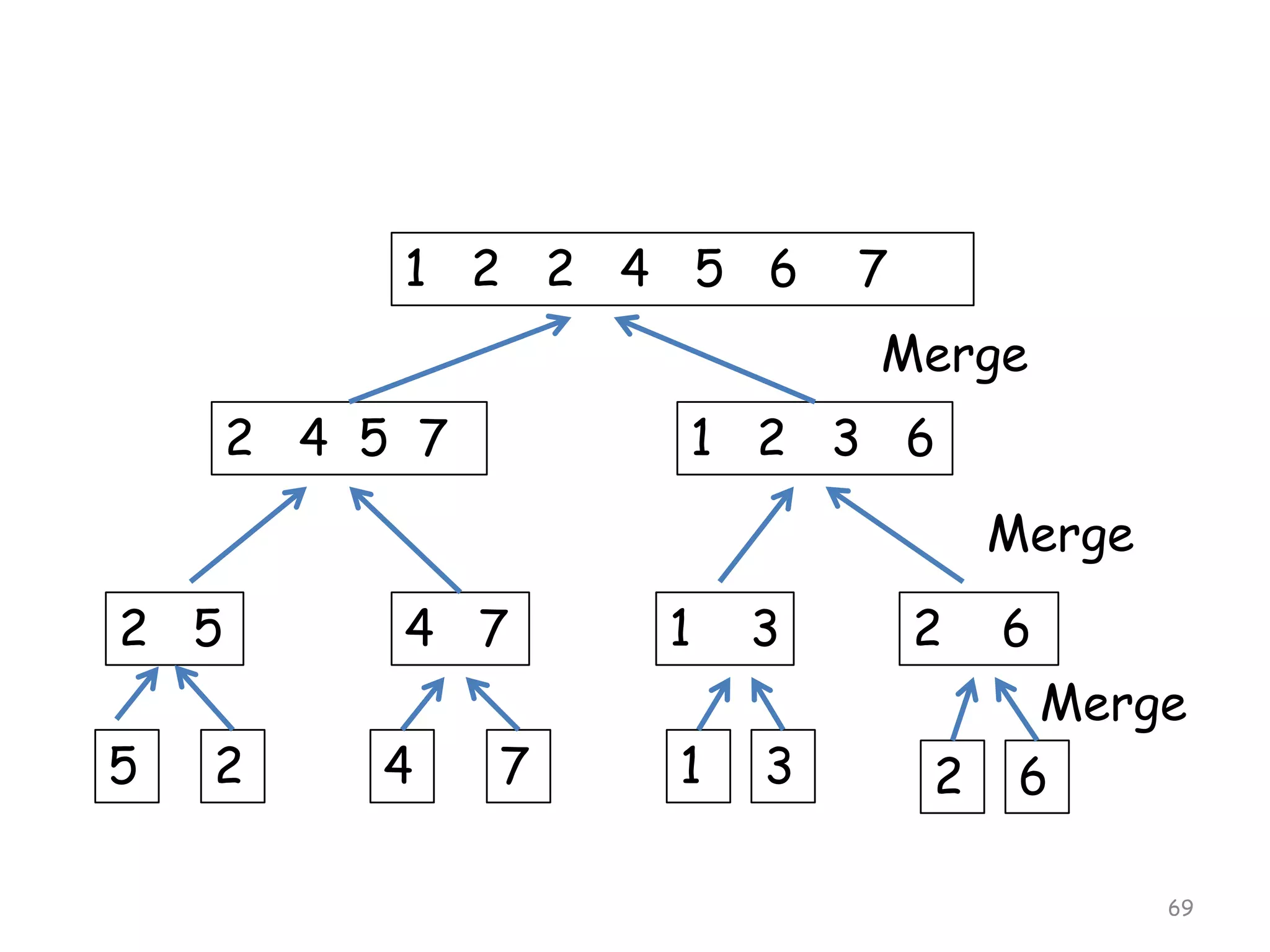
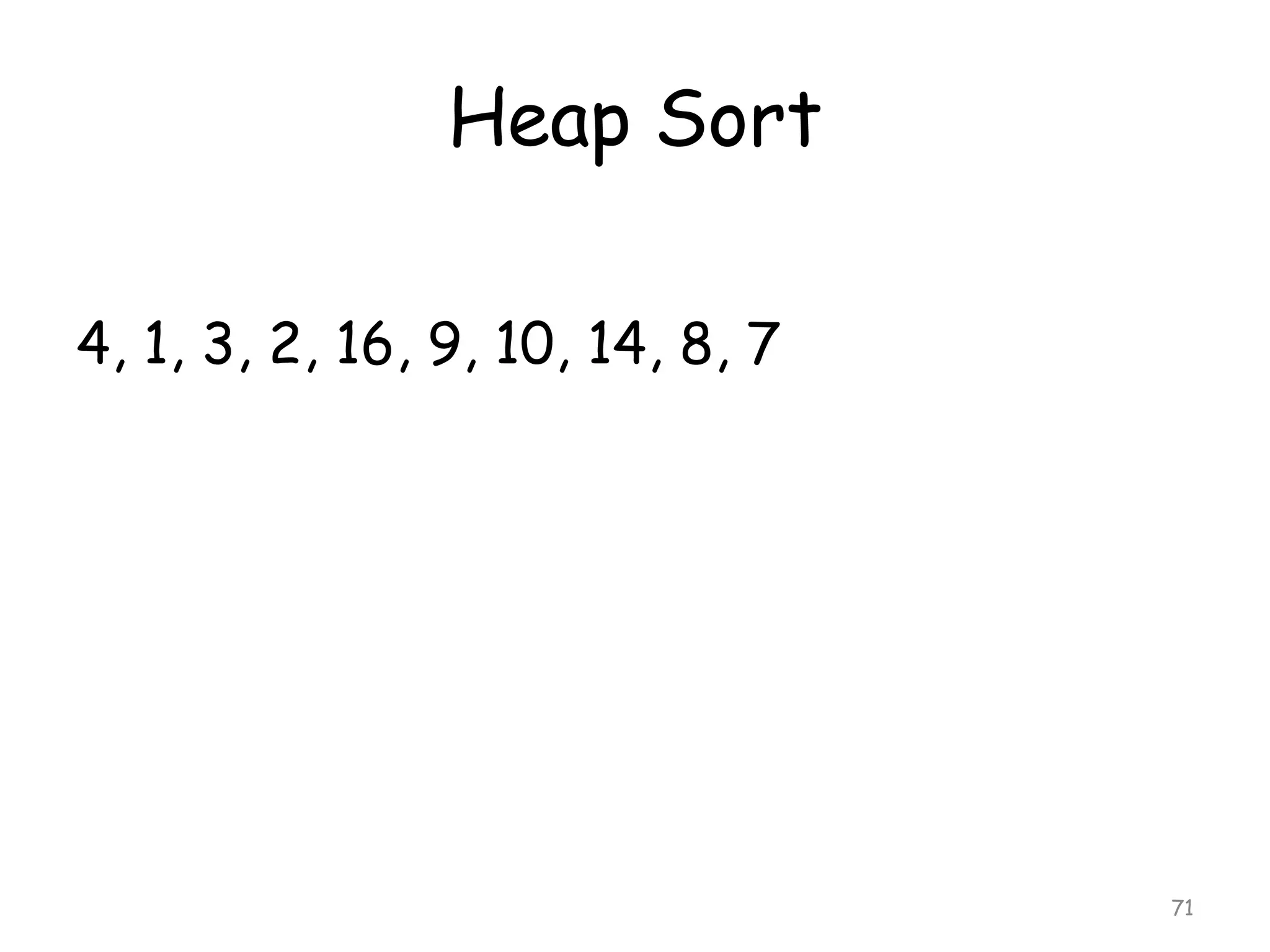
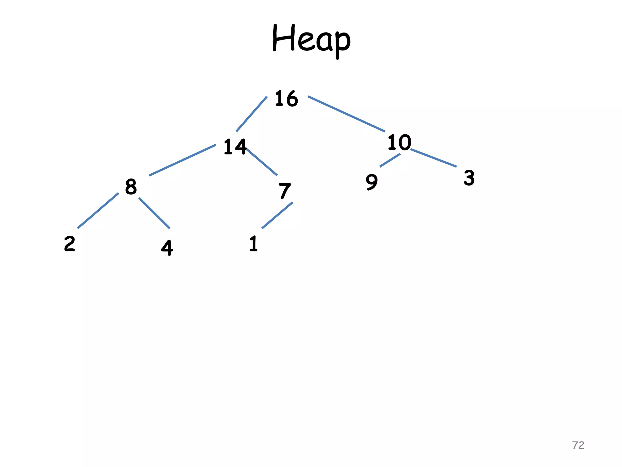

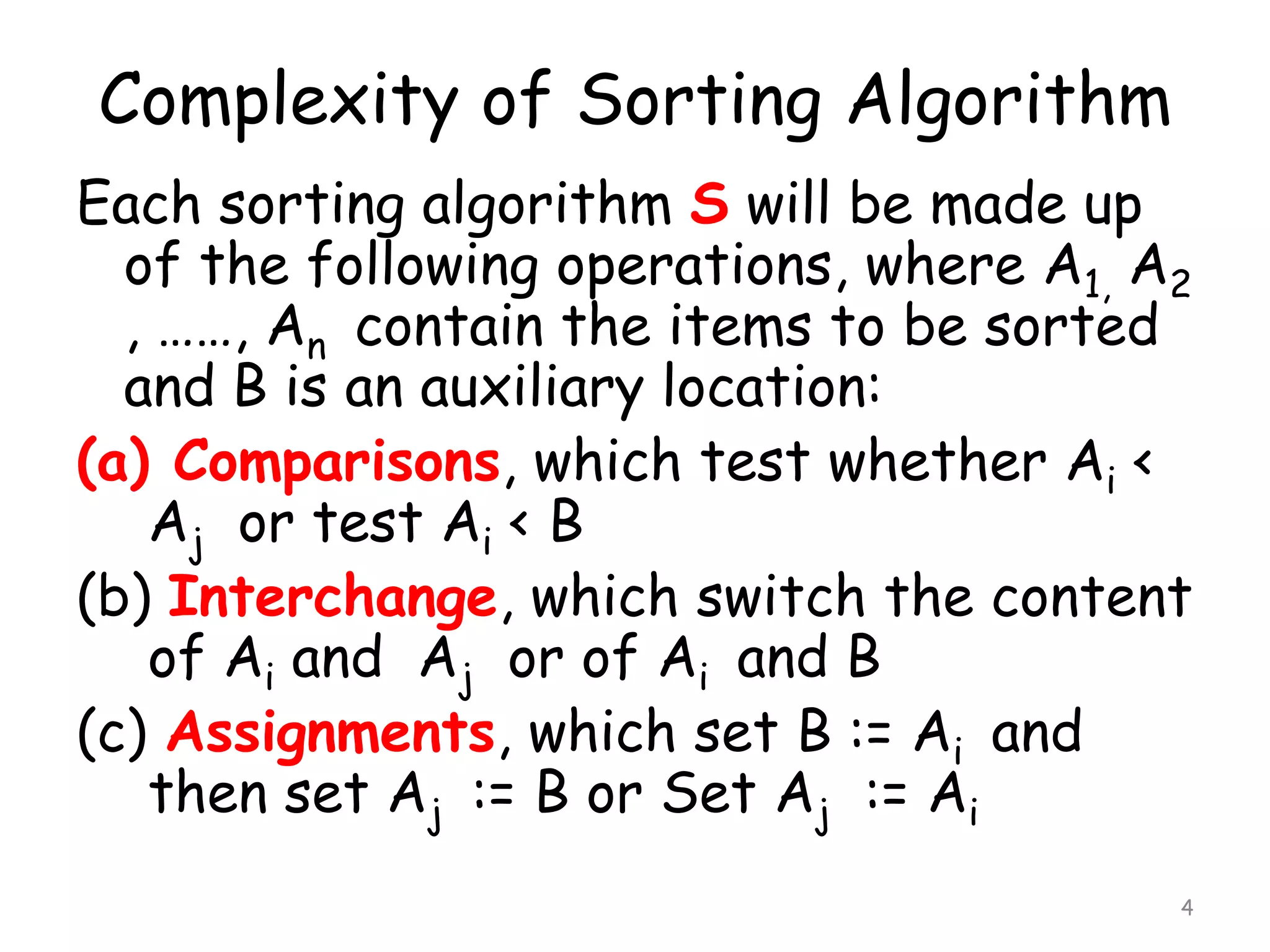
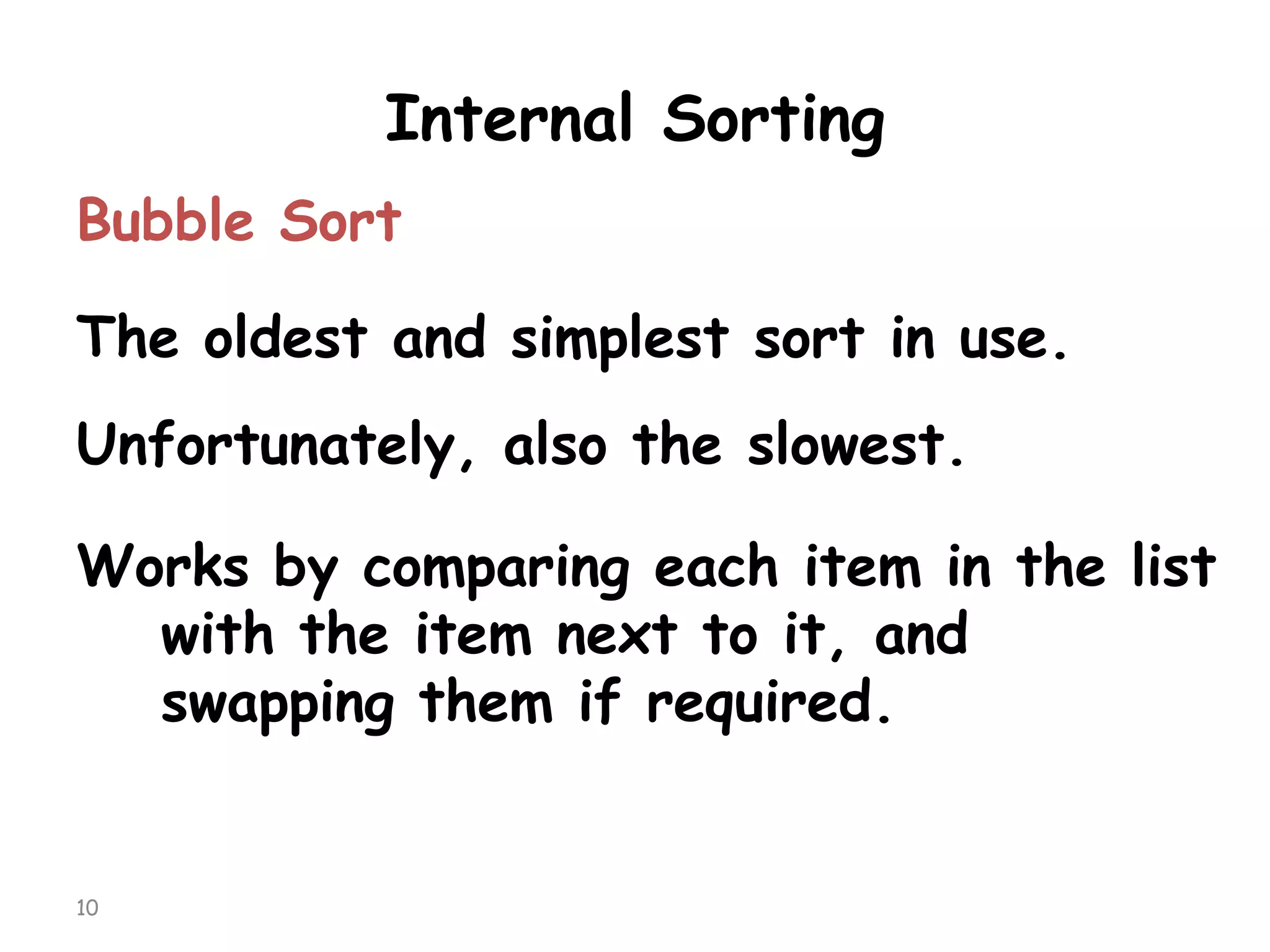
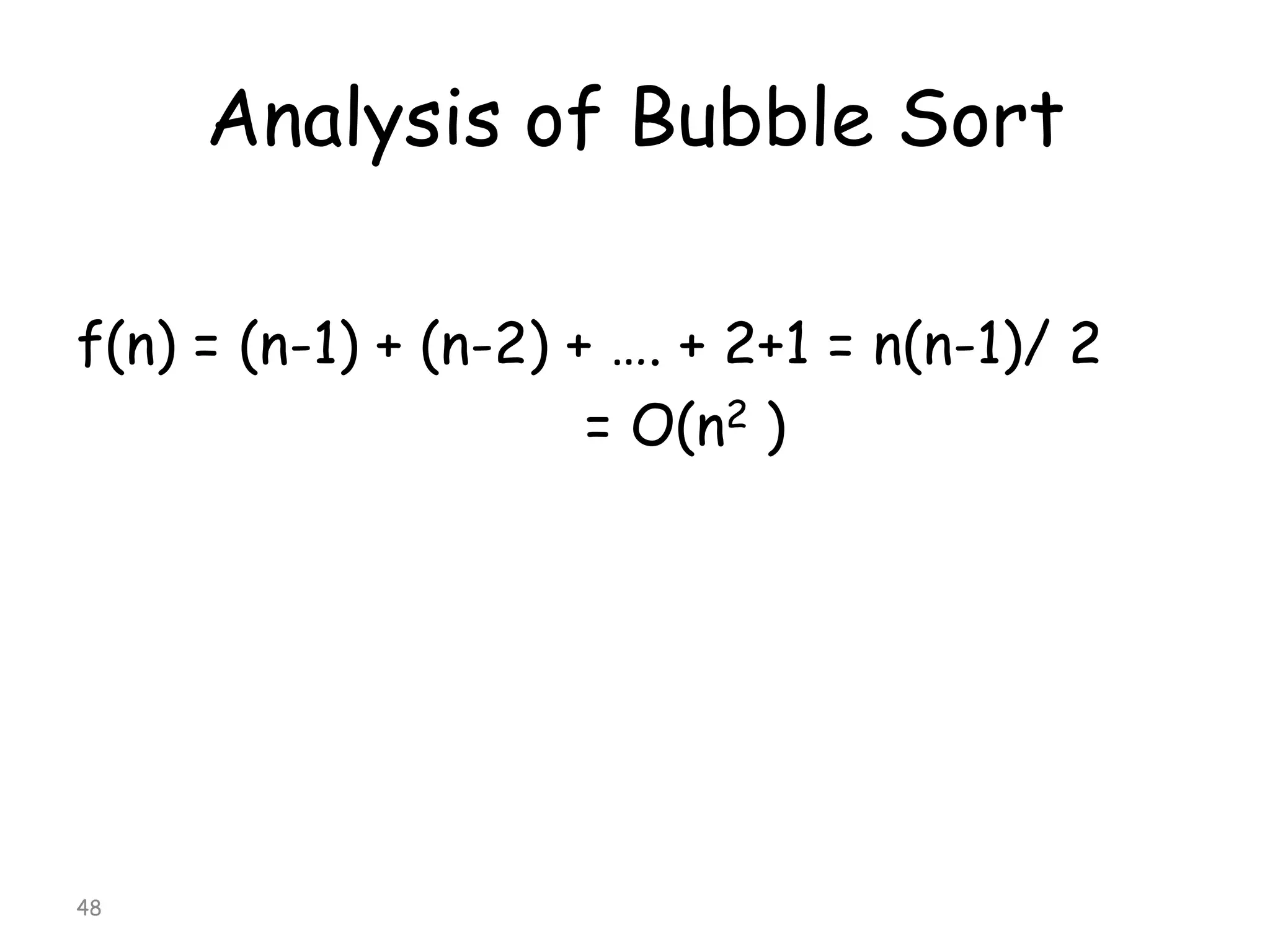
The document discusses various sorting algorithms and their complexity. It begins by defining sorting as arranging data in increasing or decreasing order. It then discusses the complexity of sorting algorithms in terms of comparisons, swaps, and assignments needed. Sorting algorithms are divided into internal sorts, which use only main memory, and external sorts, which use external storage like disks. Popular internal sorting algorithms discussed in detail include bubble sort, selection sort, insertion sort, and merge sort. Bubble sort has a time complexity of O(n2) while merge sort and quicksort have better time complexities of O(nlogn).