Downloaded 16 times


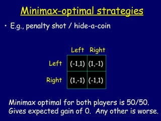
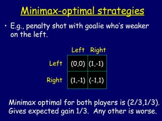
![Minimax-optimal strategies Minimax optimal strategy is a (randomized) strategy that has the best guarantee on its expected gain. [maximizes the minimum] I.e., the thing to play if your opponent knows you well. Same as our notion of a randomized strategy with a good worst-case bound. In class on Linear Programming, we saw how to solve for this using LP. polynomial time in size of matrix if use poly-time LP alg (like Ellipsoid).](https://image.slidesharecdn.com/lect1207-13658/85/lect1207-4-320.jpg)
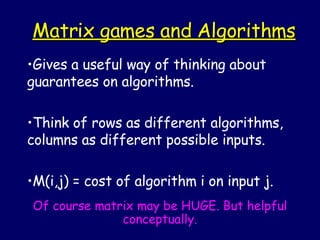
![E.g., hashing Rows are different hash functions. Cols are different sets of n items to hash. M(i,j) = #collisions incurred by alg i on set j. [alg is trying to minimize] For any row, can reverse-engineer a bad column. Universal hashing is a randomized strategy for row player. Alg player Adversary](https://image.slidesharecdn.com/lect1207-13658/85/lect1207-11-320.jpg)
![Nice proof of minimax thm (sketch) Suppose for contradiction it was false. This means some game G has V C > V R : If Column player commits first, there exists a row that gets at least V C . But if Row player has to commit first, the Column player can make him get only V R . Scale matrix so payoffs to row are in [0,1]. Say V R = V C (1- ) . V C V R](https://image.slidesharecdn.com/lect1207-13658/85/lect1207-13-320.jpg)
![Proof sketch, contd Consider repeatedly playing game G against some opponent. [think of you as row player] Use “picking a winner / expert advice” alg to do nearly as well as best fixed row in hindsight. Alg gets ¸ OPT – c*log n > OPT [if play long enough] OPT ¸ V C [Best against opponent’s empirical distribution] Alg · V R [Each time, opponent knows your randomized strategy] Contradicts assumption.](https://image.slidesharecdn.com/lect1207-13658/85/lect1207-14-320.jpg)
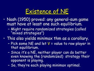
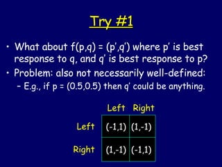
![Existence of NE Proof will be non-constructive. Unlike case of zero-sum games, we do not know any polynomial-time algorithm for finding Nash Equilibria in general-sum games. [great open problem!] Notation: Assume an nxn matrix. Use (p 1 ,...,p n ) to denote mixed strategy for row player, and (q 1 ,...,q n ) to denote mixed strategy for column player.](https://image.slidesharecdn.com/lect1207-13658/85/lect1207-23-320.jpg)
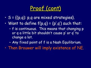
![Proof We’ll start with Brouwer’s fixed point theorem. Let S be a compact convex region in R n and let f:S ! S be a continuous function. Then there must exist x 2 S such that f(x)=x. x is called a “fixed point” of f. Simple case: S is the interval [0,1]. We will care about: S = {(p,q): p,q are legal probability distributions on 1,...,n}. I.e., S = simplex n £ simplex n](https://image.slidesharecdn.com/lect1207-13658/85/lect1207-24-320.jpg)
![Instead we will use... f(p,q) = (p’,q’) such that: q’ maximizes [(expected gain wrt p) - ||q-q’|| 2 ] p’ maximizes [(expected gain wrt q) - ||p-p’|| 2 ] p p’ Note: quadratic + linear = quadratic.](https://image.slidesharecdn.com/lect1207-13658/85/lect1207-28-320.jpg)
![Instead we will use... f(p,q) = (p’,q’) such that: q’ maximizes [(expected gain wrt p) - ||q-q’|| 2 ] p’ maximizes [(expected gain wrt q) - ||p-p’|| 2 ] p Note: quadratic + linear = quadratic. p’](https://image.slidesharecdn.com/lect1207-13658/85/lect1207-29-320.jpg)
![Instead we will use... f(p,q) = (p’,q’) such that: q’ maximizes [(expected gain wrt p) - ||q-q’|| 2 ] p’ maximizes [(expected gain wrt q) - ||p-p’|| 2 ] f is well-defined and continuous since quadratic has unique maximum and small change to p,q only moves this a little. Also fixed point = NE. (even if tiny incentive to move, will move little bit). So, that’s it!](https://image.slidesharecdn.com/lect1207-13658/85/lect1207-30-320.jpg)

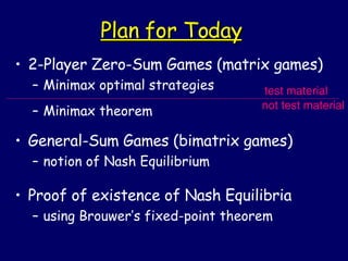
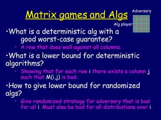
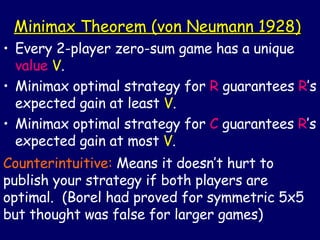
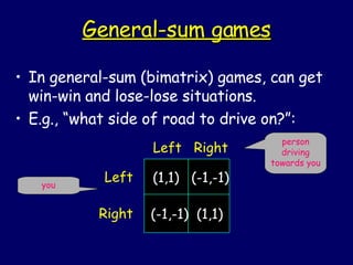
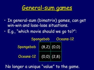
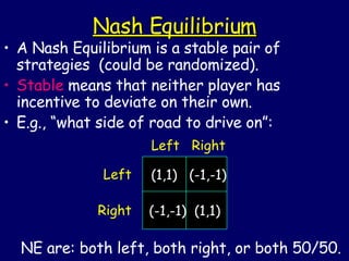
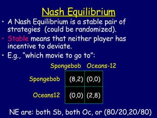
This document provides an overview of game theory concepts including: - 2-player zero-sum games and minimax optimal strategies - The minimax theorem which states that every 2-player zero-sum game has a value and optimal strategies for both players - General-sum games and the concept of a Nash equilibrium as a stable pair of strategies where neither player benefits from deviating - The proof of existence of Nash equilibria in general-sum games using Brouwer's fixed-point theorem