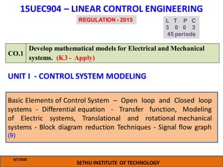
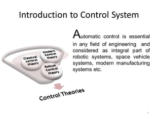
This document provides an overview of linear control engineering concepts including:
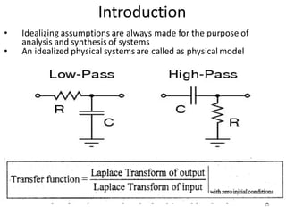
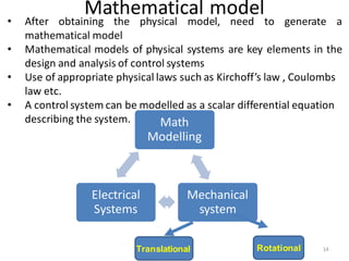
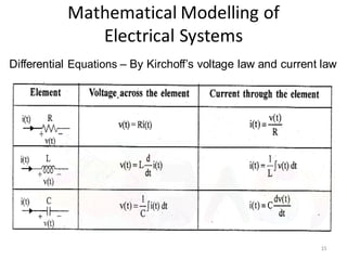
- Modeling of electrical and mechanical systems using differential equations and transfer functions. Mathematical models allow analysis of system behavior.
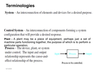
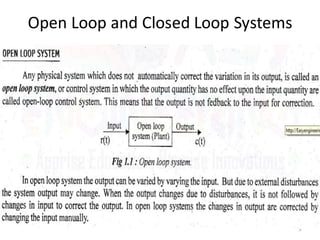
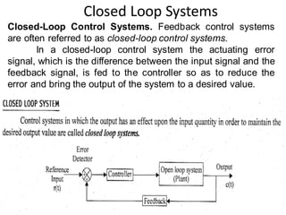
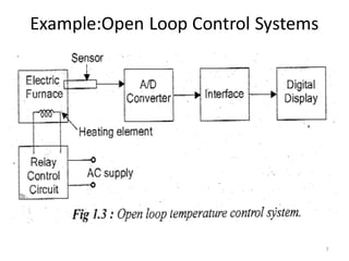
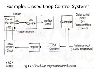
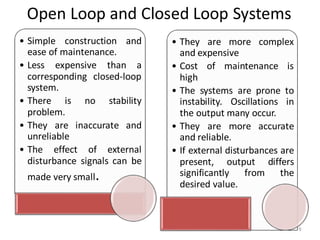
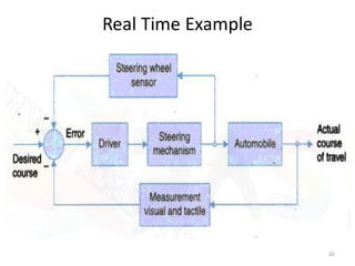
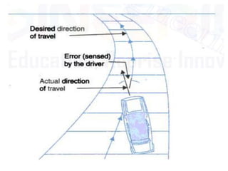
- Characteristics and examples of open-loop and closed-loop control systems. Closed-loop systems use feedback to reduce errors and improve accuracy.
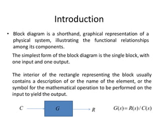
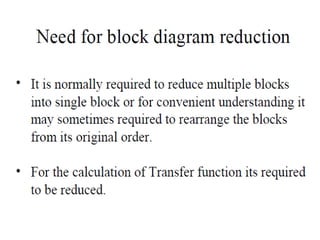
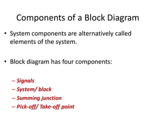
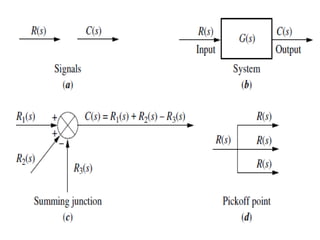
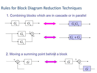
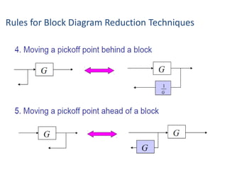
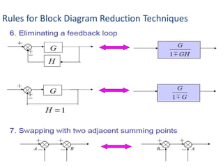
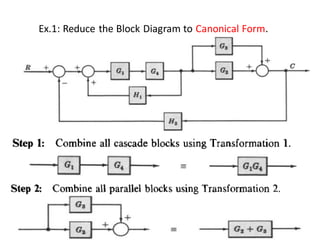
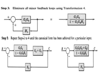
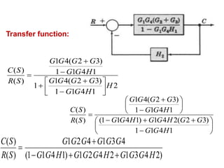
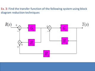
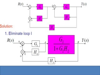
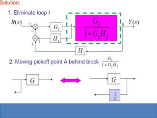
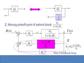
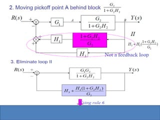
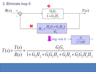
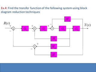
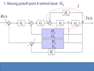
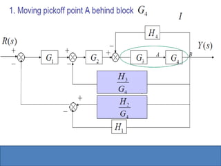
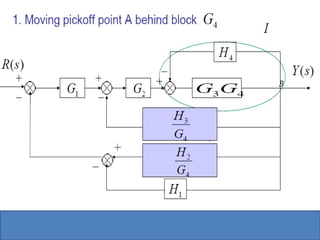
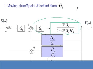
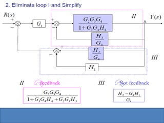
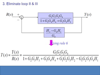
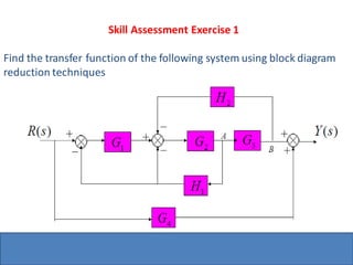
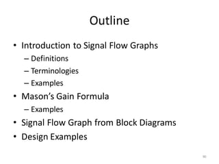
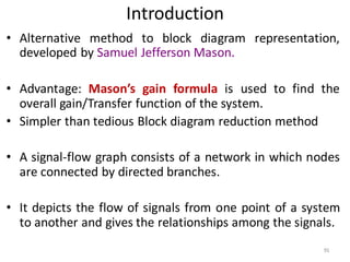
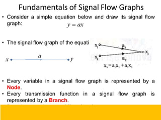
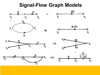
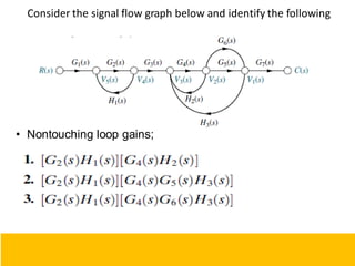
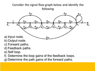
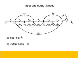
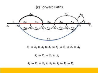
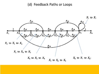
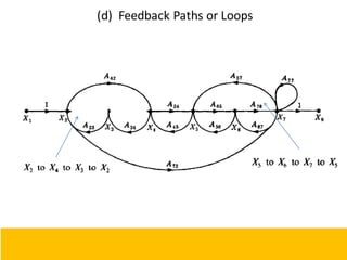
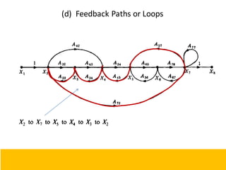
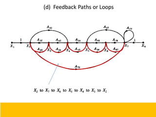
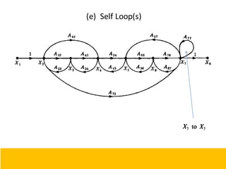
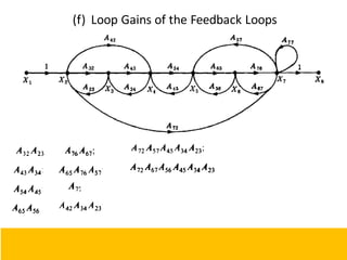
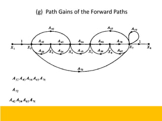
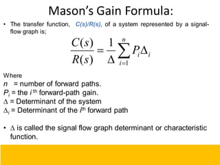
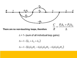
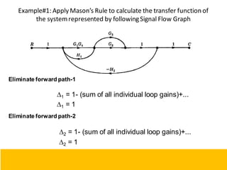
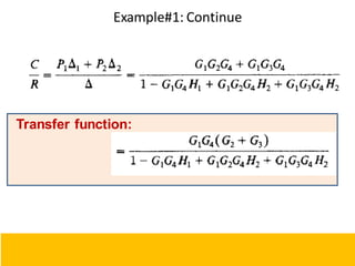
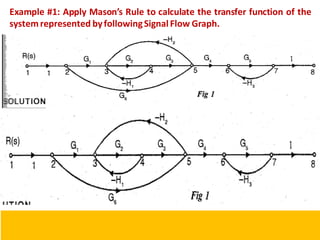
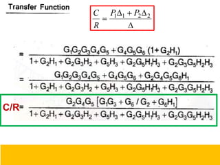
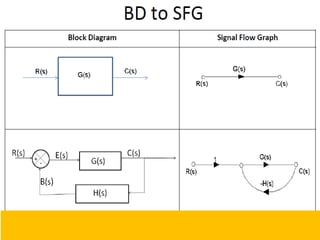
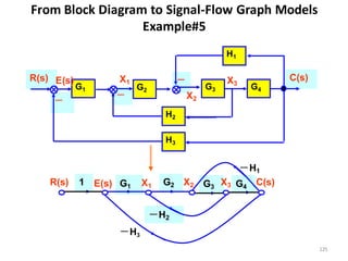
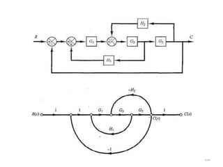
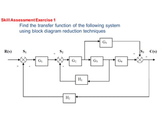
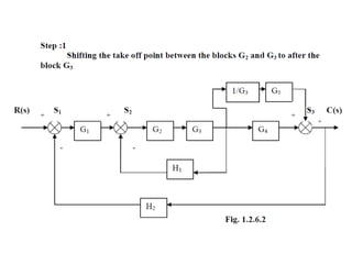
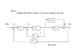
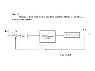
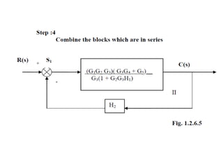
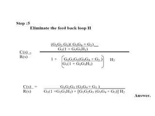
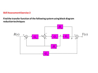
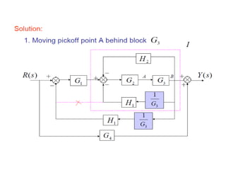
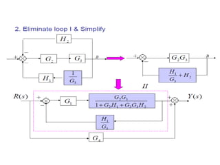
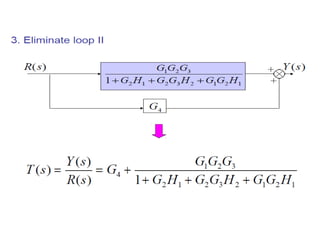
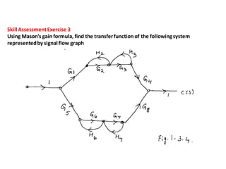
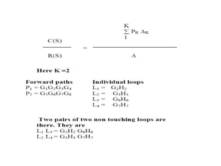
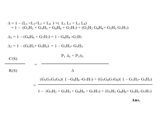
- Block diagram representation and reduction techniques to simplify analysis of multi-component systems. Signal flow graphs provide an alternative representation using Mason's gain formula.
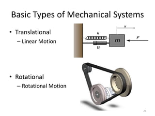
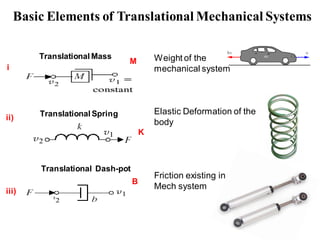
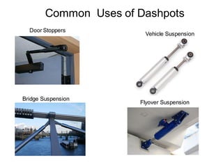
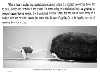
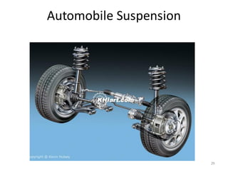
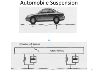
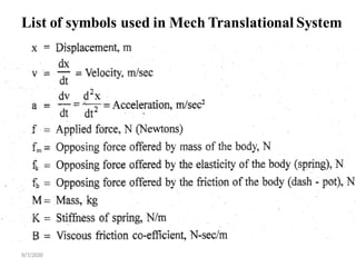
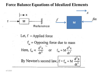
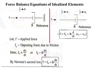
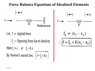
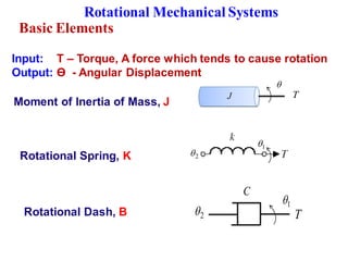
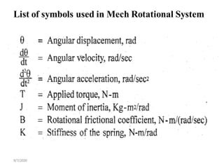
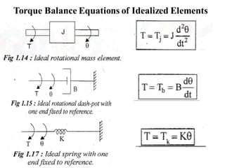
- Modeling of basic mechanical translational and rotational systems using mass, spring, damper elements and developing corresponding differential equations.
![9/7/2020
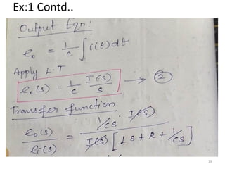
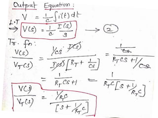
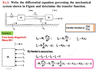
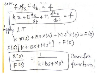
Apply L.T on force equation We know that:
[1]
Free body diagramfor
Mass M2:](https://image.slidesharecdn.com/lce-unit2ppt-221229054511-3da9dfd6/85/LCE-UNIT-2-PPT-pdf-36-320.jpg)
![9/7/2020
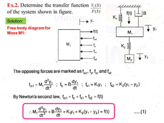
[2]](https://image.slidesharecdn.com/lce-unit2ppt-221229054511-3da9dfd6/85/LCE-UNIT-2-PPT-pdf-37-320.jpg)
![9/7/2020
[2]](https://image.slidesharecdn.com/lce-unit2ppt-221229054511-3da9dfd6/85/LCE-UNIT-2-PPT-pdf-38-320.jpg)
![9/7/2020
[2]
Free body diagramfor
Mass M2:](https://image.slidesharecdn.com/lce-unit2ppt-221229054511-3da9dfd6/85/LCE-UNIT-2-PPT-pdf-40-320.jpg)
![9/7/2020
[3]
Transfer
Function:](https://image.slidesharecdn.com/lce-unit2ppt-221229054511-3da9dfd6/85/LCE-UNIT-2-PPT-pdf-41-320.jpg)
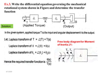
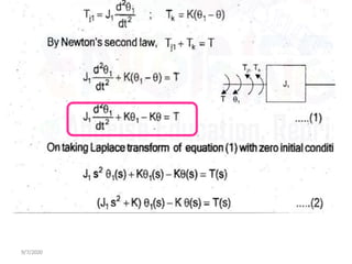
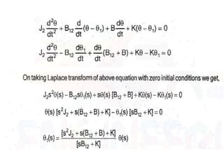
![9/7/2020
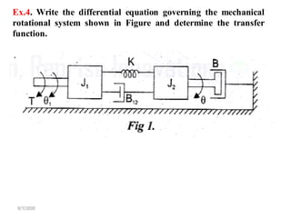
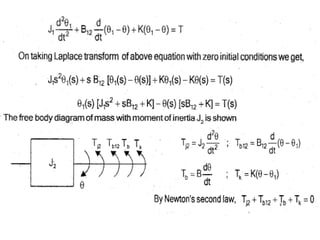
Free body diagramfor Moment
of Inertia J2:
[3]](https://image.slidesharecdn.com/lce-unit2ppt-221229054511-3da9dfd6/85/LCE-UNIT-2-PPT-pdf-50-320.jpg)
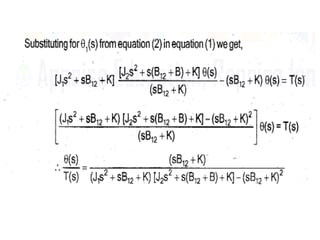
![9/7/2020
[4]
Transfer
Function:](https://image.slidesharecdn.com/lce-unit2ppt-221229054511-3da9dfd6/85/LCE-UNIT-2-PPT-pdf-51-320.jpg)