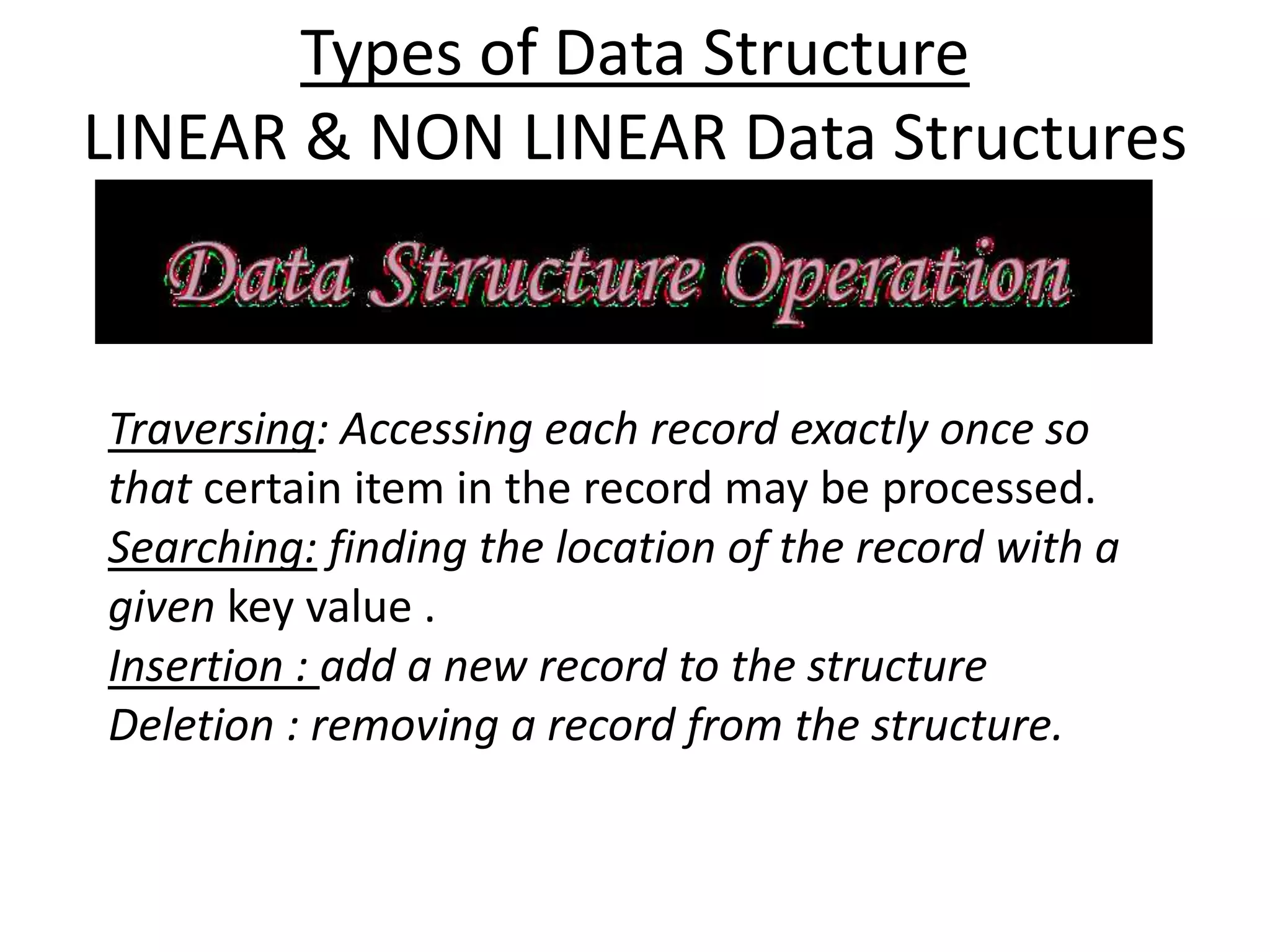
The document discusses different data structures like arrays, stacks, queues, linked lists, trees, graphs. It provides definitions of each data structure and describes their common operations like traversing, searching, insertion, deletion. It also includes algorithms for operations on linear arrays, stacks, queues and priority queues. Implementation of different data structures and their applications are explained with examples.

1. MODULE-1
Concept Of Data Structures

2. It is a logical way of storing data and it also define
mechanism of retrieve data.
Characteristics of a Data Structure
• Correctness − Data structure implementation
should implement its interface correctly.
• Time Complexity − Running time or the
execution time of operations of data structure
must be as small as possible.
• Space Complexity − Memory usage of a data
structure operation should be as little as possible.

3. Need for Data Structure
As applications are getting complex and data rich,
there are three common problems that applications
face now-a-days.
• Data Search − Consider an inventory of 1 million(106)
items of a store. If the application is to search an item,
it has to search an item in 1 million(106) items every
time slowing down the search. As data grows, search
will become slower.
• Processor Speed − Processor speed although being
very high, falls limited if the data grows to billion
records.
• Multiple Requests − As thousands of users can search
data simultaneously on a web server, even the fast
server fails while searching the data.

4. Types of Data Structure
LINEAR & NON LINEAR Data Structures
Traversing: Accessing each record exactly once so
that certain item in the record may be processed.
Searching: finding the location of the record with a
given key value .
Insertion : add a new record to the structure
Deletion : removing a record from the structure.

5. 1.Array
2.Stack
3.Queue
4.Linked List

6. An array is a collection of
homogeneous type of data
elements. An array is consisting
of a collection of elements .

7. 1.Traversing
2.Search
3.Insertion
4.Deletion
5.Sorting
6.Merging

8. Representation of array in memory

9. A Stack is a list of elements in which an
element may be inserted or deleted at one
end which is known as TOP of the stack.
Operations Performed on stack
• Push: add an element in stack
• Pop: remove an element in stack

10. Stack Representation

11. A queue is a linear list of element in which
insertion can be done at one end which is
known as front and deletion can be done
which is known as rear.
Operations Performed on Queue
• Insertion : add a new element in queue
• Deletion: Removing an element in queue

12. Representation of Queue
55
65 75

13. A Linked list is a linear collection of data elements.
It has two part one is info and other is link part.
Info part gives information and link part is
address of next node.
Operations Perfomed on Linked List
1.Traversing
2.Searching
3.Insertion
4.Deletion

14. Linked Representation

15. 1.Tree
2.Graph
1.TREE
In computer science, a tree is a widely-used data
structure that emulates a hierarchical tree
structure with a set of linked nodes.

16. 1.Insertion
2.Deletion
3.Searching

17. A graph data structure may also associate to
each edge some edge value, such as a
symbolic label or a numeric attribute (cost,
capacity, length, etc.).
Operations Performed on graph
1.Searching
2.Insertion
3.Deletion

18. Graph Representation

19. Array
Definition has described in slide
6.

20. Linear Arrays
A linear array is a list of a finite number of n
homogeneous data elements ( that is data
elements of the same type) such that
– The elements of the arrays are referenced
respectively by an index set consisting of n
consecutive numbers
– The elements of the arrays are
storedrespectively in successive memory
locations

21. The number n of elements is called the
length or size of the array.
• The index set consists of the integer 1,
2, … n
• Length or the number of data elements of
the array can be obtained from the index
set by
Length = UB – LB + 1 where UB is the
largest index called the upper bound and
LB is the smallest index called the lower
bound of the arrays

22. • Element of an array A may be denoted
by
– Subscript notation A1, A2, , …. , An
– Parenthesis notation A(1), A(2), …. , A(n)
– Bracket notation A[1], A[2], ….. , A[n]
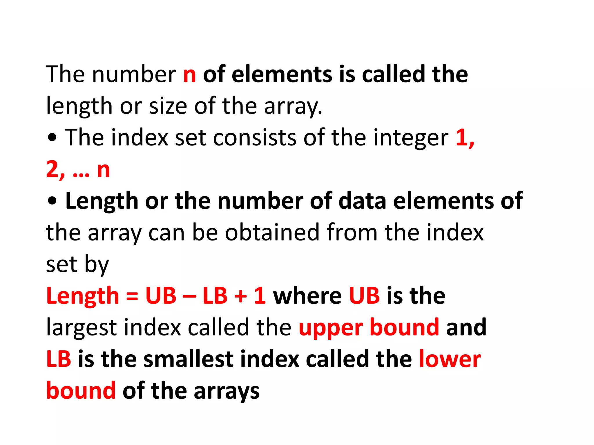
• The number K in A[K] is called subscript
or an index and A[K] is called a
subscripted variable

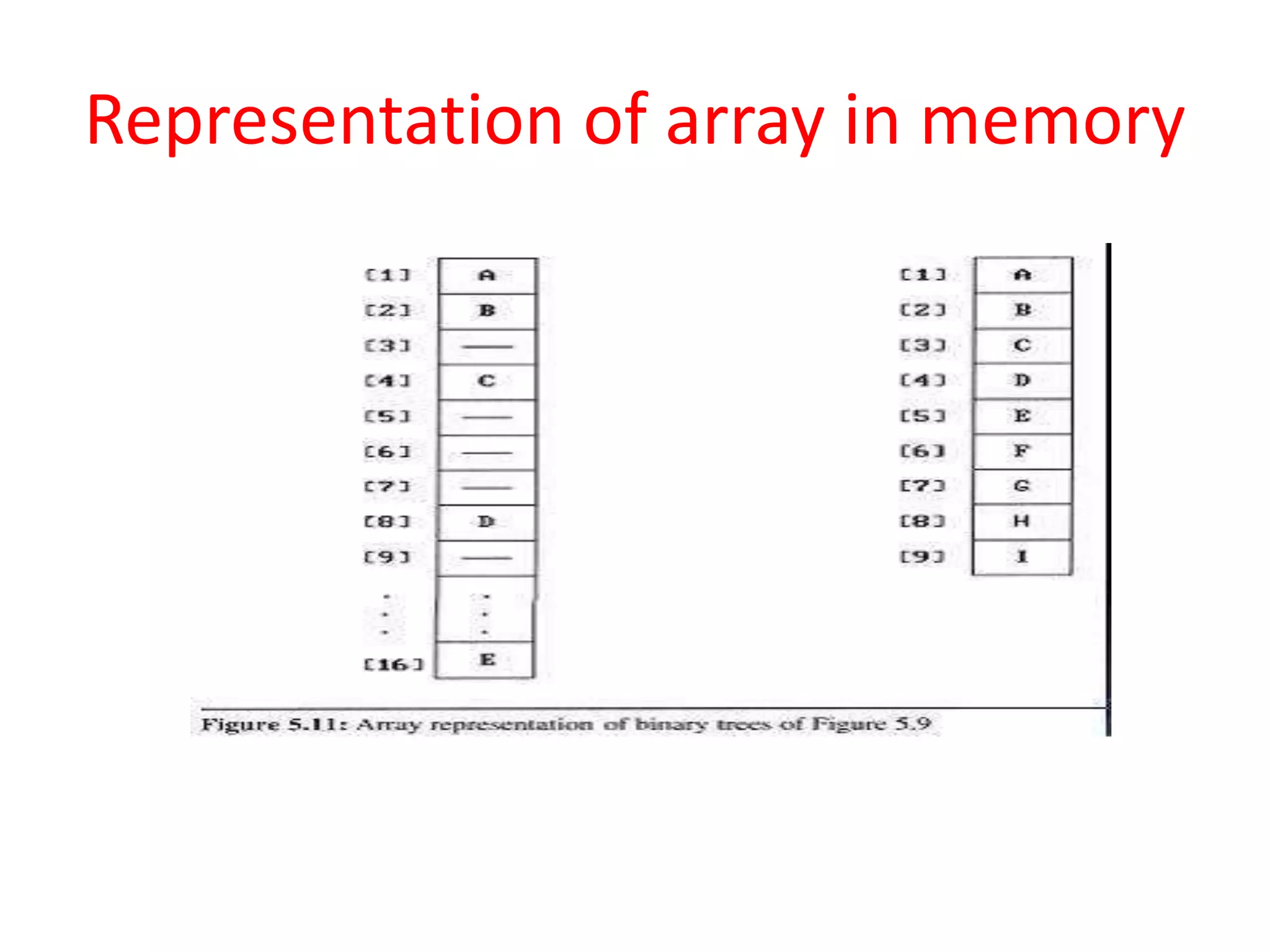
23. Representation of Linear Array in Memory
• Let LA be a linear array in the memory of the
computer
• LOC(LA[K]) = address of the element LA[K] of
the array LA
• The element of LA are stored in the successive
memory cells
• Computer does not need to keep track of
the address of every element of LA, but
need to track only the address of the first
element of the array denoted by Base(LA)
called the base address of LA

24. Insertion Algorithm
INSERT (LA, N , K , ITEM) [LA is a linear array with N
elements and K is a positive integers such that K ≤ N.
This algorithm inserts an element ITEM into the K th
position in LA ]
1. [Initialize Counter] Set J := N
2. Repeat Steps 3 and 4 while J ≥ K
3. [Move the Jth element downward ] Set LA[J + 1]:= LA[J]
4. [Decrease Counter] Set J := J -1
5 [Insert Element] Set LA[K] := ITEM
6. [Reset N] Set N := N +1;
7. Exit

25. Deletion Algorithm
DELETE (LA, N , K , ITEM) [LA is a linear array with N
elements and K is a positive integers such that K ≤
N. This algorithm deletes Kth element from LA ]
1. Set ITEM := LA[K]
2. Repeat for J = K+1 to N:[Move the Jth element
upward] Set LA[J-1] :=LA[J]
3. [Reset the number N of elements] Set N := N - 1;
4. Exit

26. Two-Dimensional Array
• A Two-Dimensional m x n array A is a
collection of m . n data elements such that
each element is specified by a pair of integers
(such as J, K) called subscripts with property
that 1 ≤ J ≤ m and 1 ≤ K ≤ n.
• The element of A with first subscript Jand
second subscript K will be denoted by AJ,K or
A[J][K].

27. 2D Arrays
The elements of a 2-dimensional array
a is shown as below
• a[0][0] a[0][1] a[0][2] a[0][3]
• a[1][0] a[1][1] a[1][2] a[1][3]
• a[2][0] a[2][1] a[2][2] a[2][3]

28. STACK
• Stack is an abstract data type with bounded
(predefined) capacity. It is a simple
data structure that allows adding and removing
elements in a particular order.
• Every time an element is added, it goes on the
top of the stack, the only element that can be
removed is the element that was at the top of
the stack, just like a pile of objects.

29. Stack Representation

30. Basic Operations
• Stack operations may involve initializing the stack, using it and
then de-initializing it. Apart from these basic stuffs, a stack is
used for the following two primary operations −
• push() − Pushing (storing) an element on the stack.
• pop() − Removing (accessing) an element from the stack.
• To use a stack efficiently, we need to check the status of stack
as well. For the same purpose, the following functionality is
added to stacks
• isFull() − check if stack is full.
• isEmpty() − check if stack is empty.

31. Algorithm for PUSH Operation
begin procedure push: stack, data
if stack is full
return null
endif
top ← top + 1
stack[top] ← data
end procedure

32. Algorithm for Pop Operation
begin procedure
pop: stack
if stack is empty
return null
endif
data ← stack[top]
top ← top – 1
return data
end procedure

33. QUEUE
• Queue is also an abstract data type or a linear
data structure, in which the first element is
inserted from one end called REAR(also called
tail), and the deletion of existing element
takes place from the other end called as
FRONT(also called head).
• This makes queue as FIFO(First in First Out)
data structure, which means that element
inserted first will also be removed first.

34. Basic Operations
• Queue operations may involve initializing or defining
the queue, utilizing it, and then completely erasing it
from the memory.
operations associated with queues −
• enqueue() − add (store) an item to the queue.
• dequeue() − remove (access) an item from the queue.
• Few more functions are required to make the above-
mentioned queue operation efficient.These are −
• isfull() − Checks if the queue is full.
• isempty() − Checks if the queue is empty.

35. Algorithm for enqueue Operation
procedure enqueue(data)
if queue is full
return overflow
endif
rear ← rear + 1
queue[rear] ← data
return true
end procedure

36. Algorithm for dequeue Operation
procedure dequeue
if queue is empty
return underflow
end if
data = queue[front]
front ← front + 1
return true
end procedure

37. Drawback of Linear Queue
Once the queue is full, even though
few elements from the front are
deleted and some occupied space is
relieved, it is not possible to add
anymore new elements, as the rear
has already reached the Queue’s rear
most position

38. Circular Queue
• This queue is not linear but
circular.
• Its structure can be like the
following figure:
• In circular queue, once the
Queue is full the "First" element of
the Queue becomes the"Rear"
most element, if and only if
the"Front"has moved forward.
otherwise it will again be a "Queue
overflow" state.

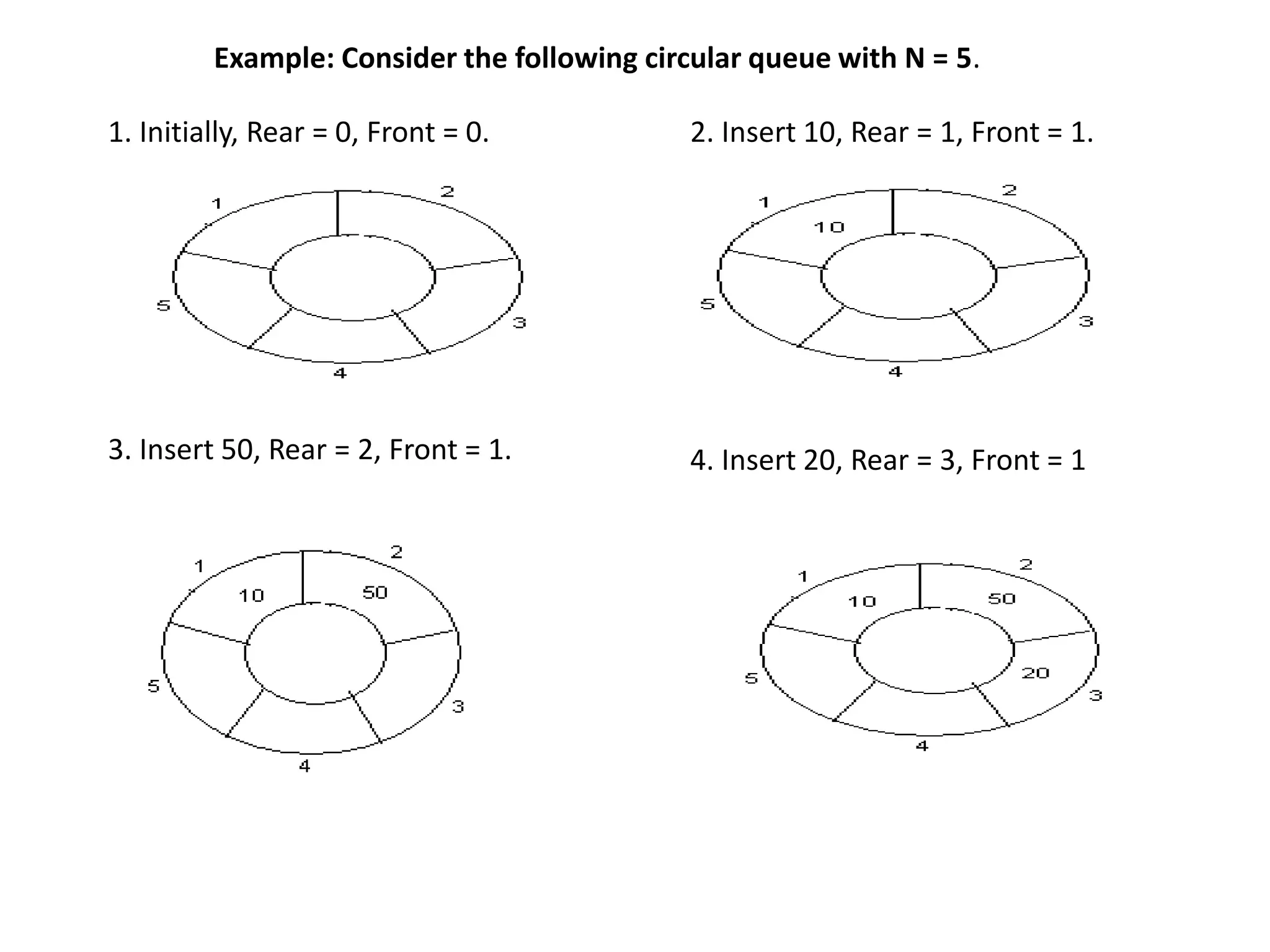
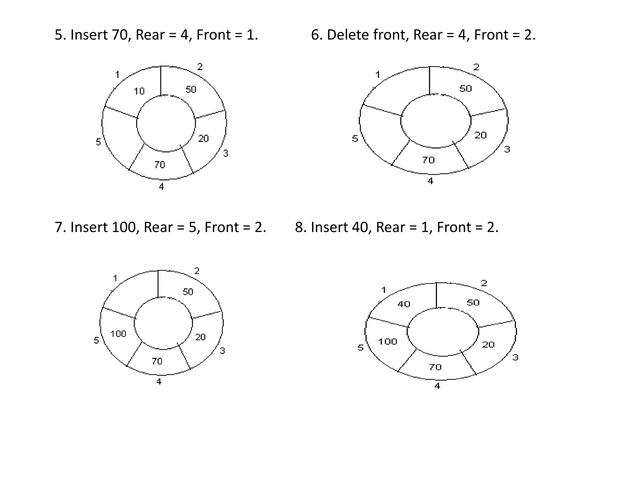
39. Algorithms for Insert and Delete
Operations in Circular Queue
For Insert Operation
Insert-Circular-Q(CQueue, Rear, Front, N, Item)
CQueue is a circular queue where to store data. Rear represents the location
in which the data element is to be inserted and Front represents the
location from which the data element is to be removed. Here N is the
maximum size of CQueue and finally, Item is the new item to be added.
Initailly Rear = 0 and Front = 0.
1. If Front = 0 and Rear = 0 then Set Front := 1 and go to step 4.
2. If Front =1 and Rear = N or Front = Rear + 1
then Print: “Circular Queue Overflow” and Return.
3. If Rear = N then Set Rear := 1 and go to step 5.
4. Set Rear := Rear + 1
5. Set CQueue [Rear] := Item.
6. Return

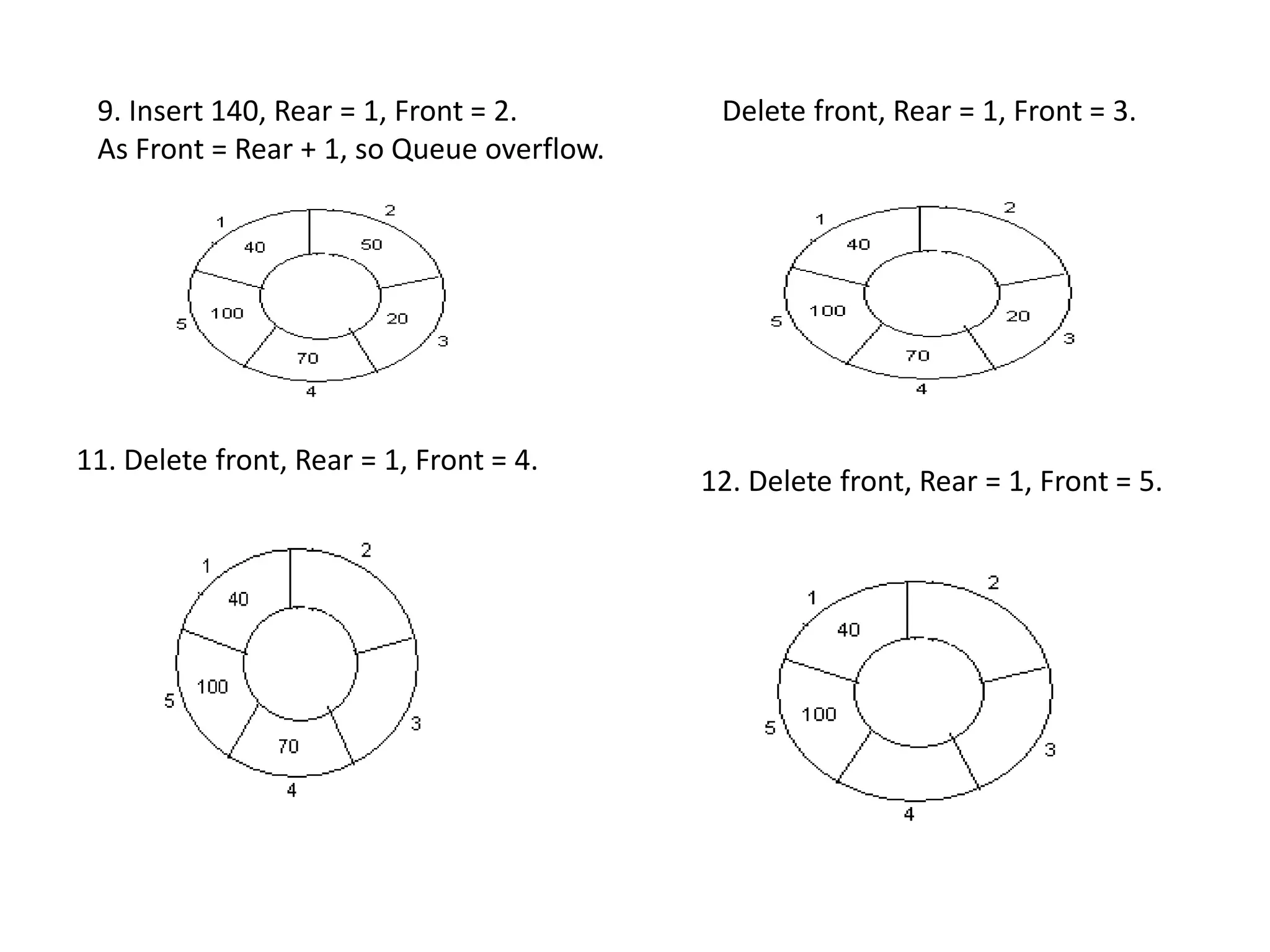
40. For Delete Operation
Delete-Circular-Q(CQueue, Front, Rear, Item)
Here, CQueue is the place where data are stored. Rear represents the
location in which the data element is to be inserted and Front
represents the location from which the data element is to be
removed. Front element is assigned to Item.
Initially, Front = 1.
1. If Front = 0 then
Print: “Circular Queue Underflow” and Return. /*..Delete without
Insertion
2. Set Item := CQueue [Front]
3. If Front = N then Set Front = 1 and Return.
4. If Front = Rear then Set Front = 0 and Rear = 0 and Return.
5. Set Front := Front + 1
6. Return.

41. Example: Consider the following circular queue with N = 5.
1. Initially, Rear = 0, Front = 0. 2. Insert 10, Rear = 1, Front = 1.
3. Insert 50, Rear = 2, Front = 1. 4. Insert 20, Rear = 3, Front = 1

42. 5. Insert 70, Rear = 4, Front = 1. 6. Delete front, Rear = 4, Front = 2.
7. Insert 100, Rear = 5, Front = 2. 8. Insert 40, Rear = 1, Front = 2.

43. 9. Insert 140, Rear = 1, Front = 2.
As Front = Rear + 1, so Queue overflow.
Delete front, Rear = 1, Front = 3.
11. Delete front, Rear = 1, Front = 4.
12. Delete front, Rear = 1, Front = 5.

44. Priority Queue

45. Priority Queue
• A priority queue is a data structure for
maintaining a set S of elements, each with
an associated value called a key.
• Heap can be used to implement a priority
queue.
There are two kinds of priority queue
• max-priority queue
• min-priority queue

46. Applications of priority queue
• Job scheduling on a shared computer
• Event-driven simulation
******************************
• You will still remove from front of queue, but
insertions are governed by a priority. But, we
want to insert quickly. Must go into proper
position.

47. Implementation of Priority Queues
Implemented using heaps and leftist trees
• Heap is a complete binary tree that is
efficiently stored using the array-based
representation
• Leftist tree is a linked data structure suitable
for the implementation of a priority queue