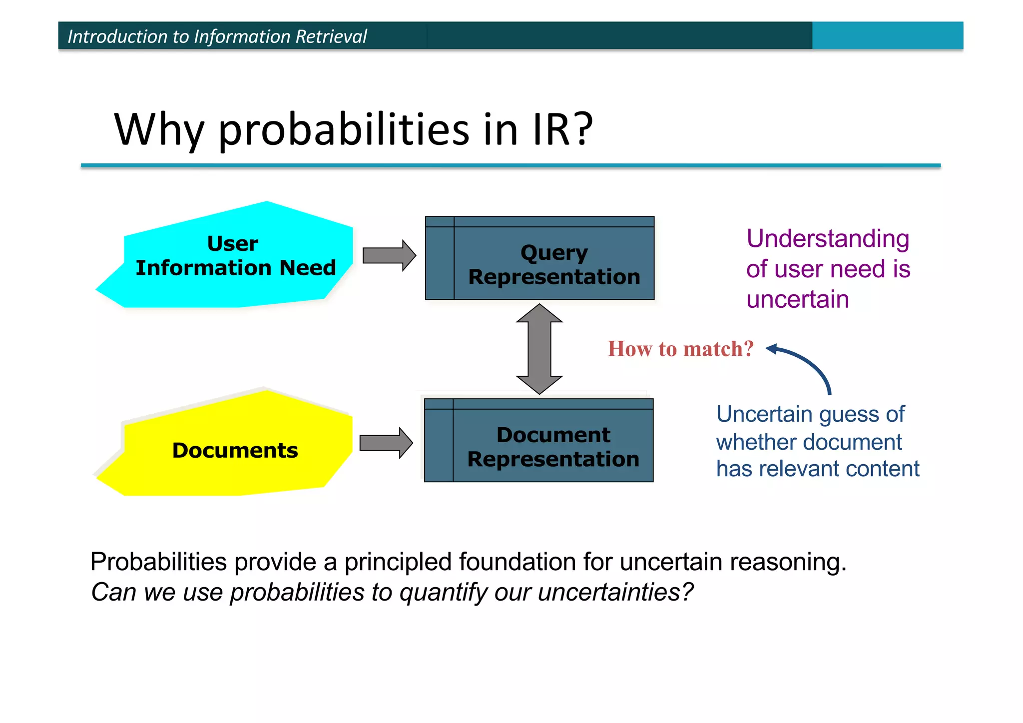
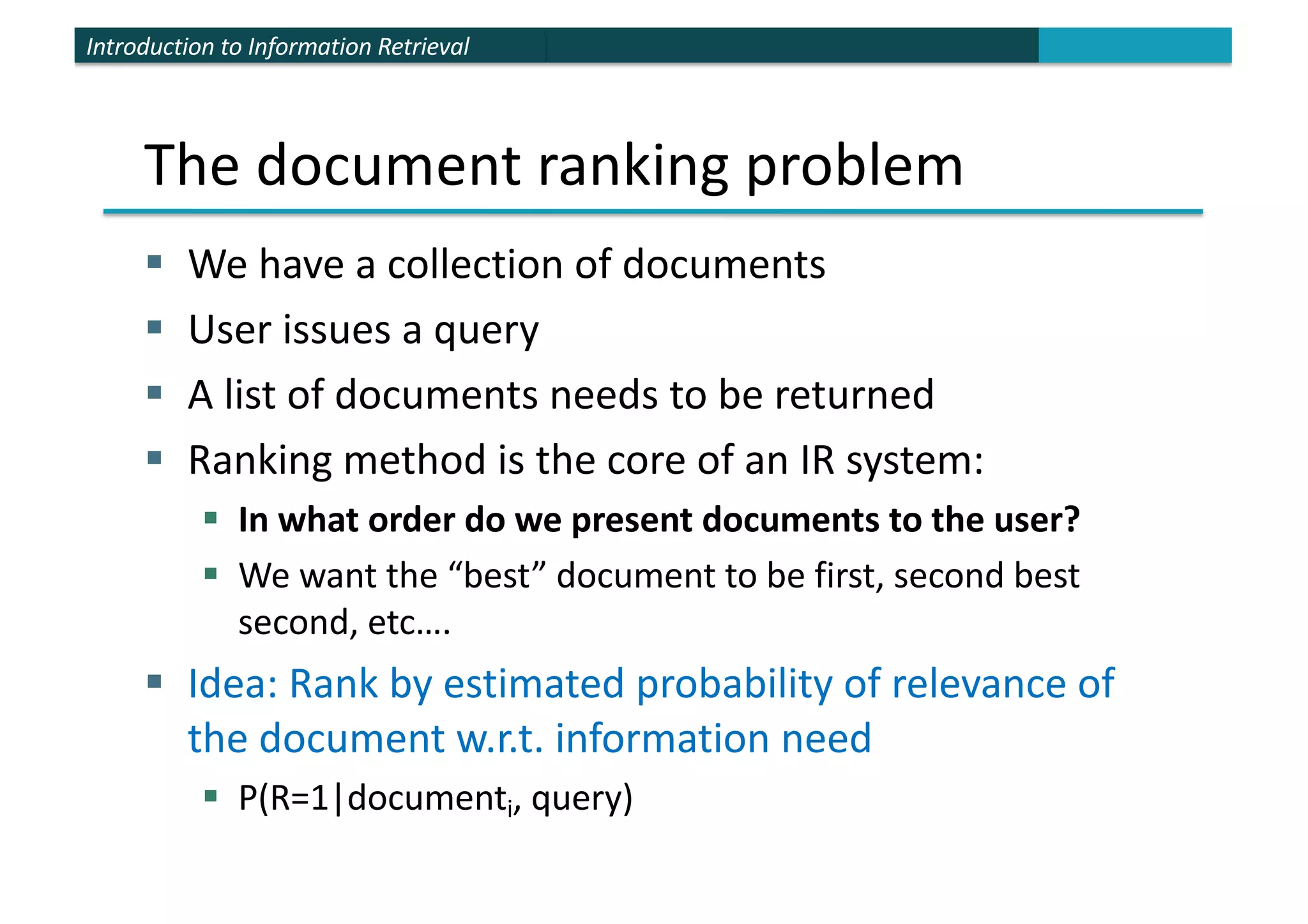
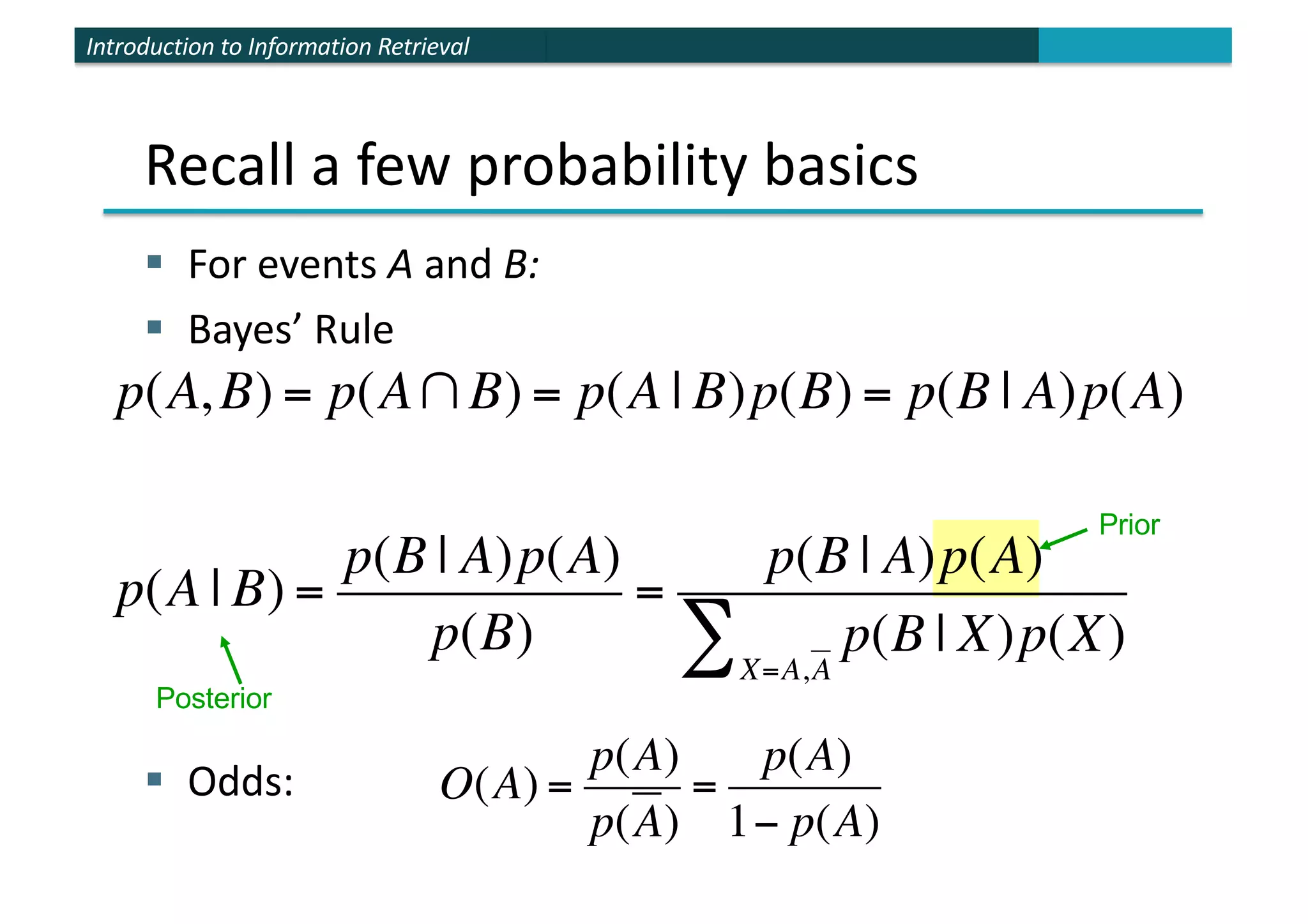
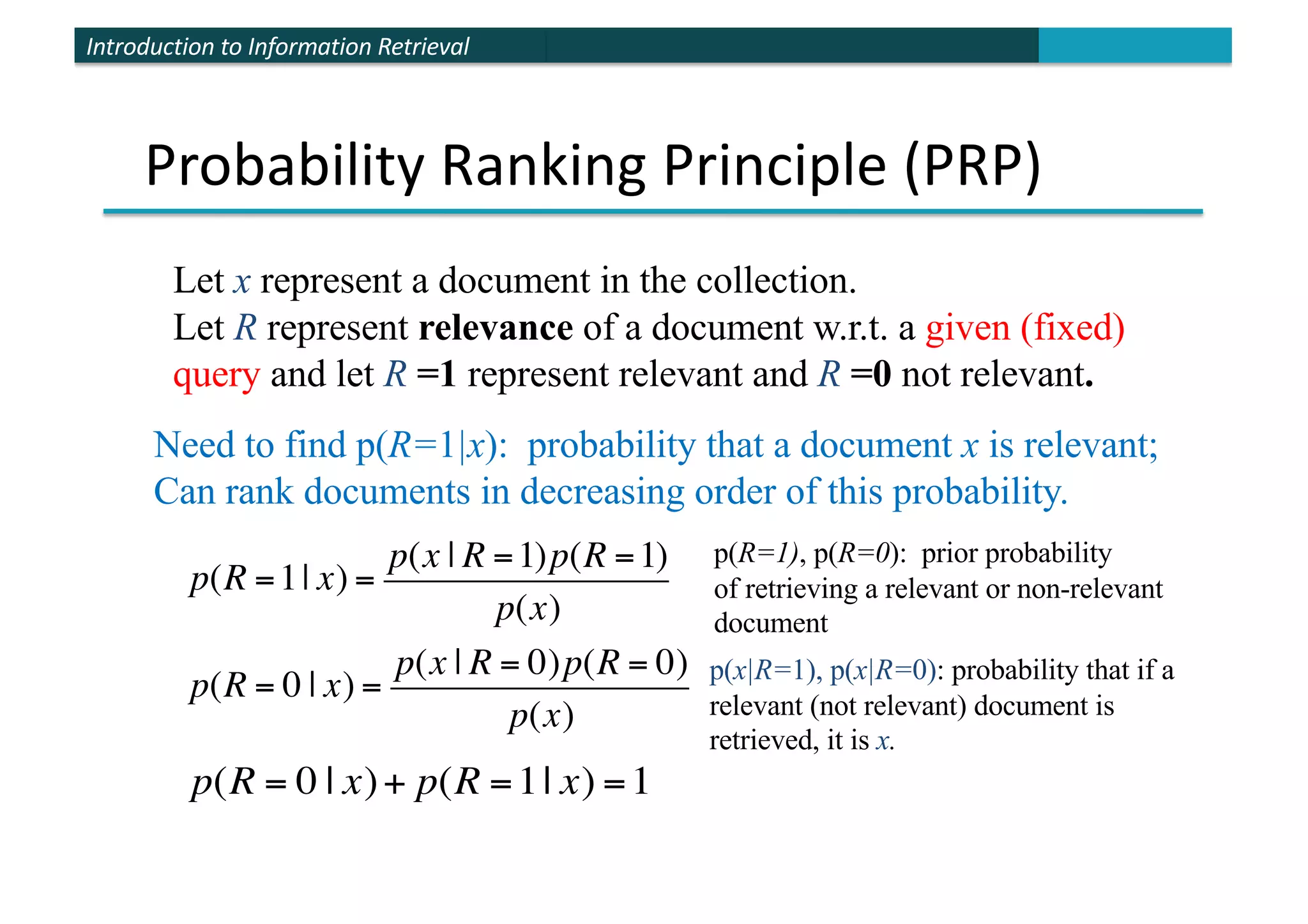
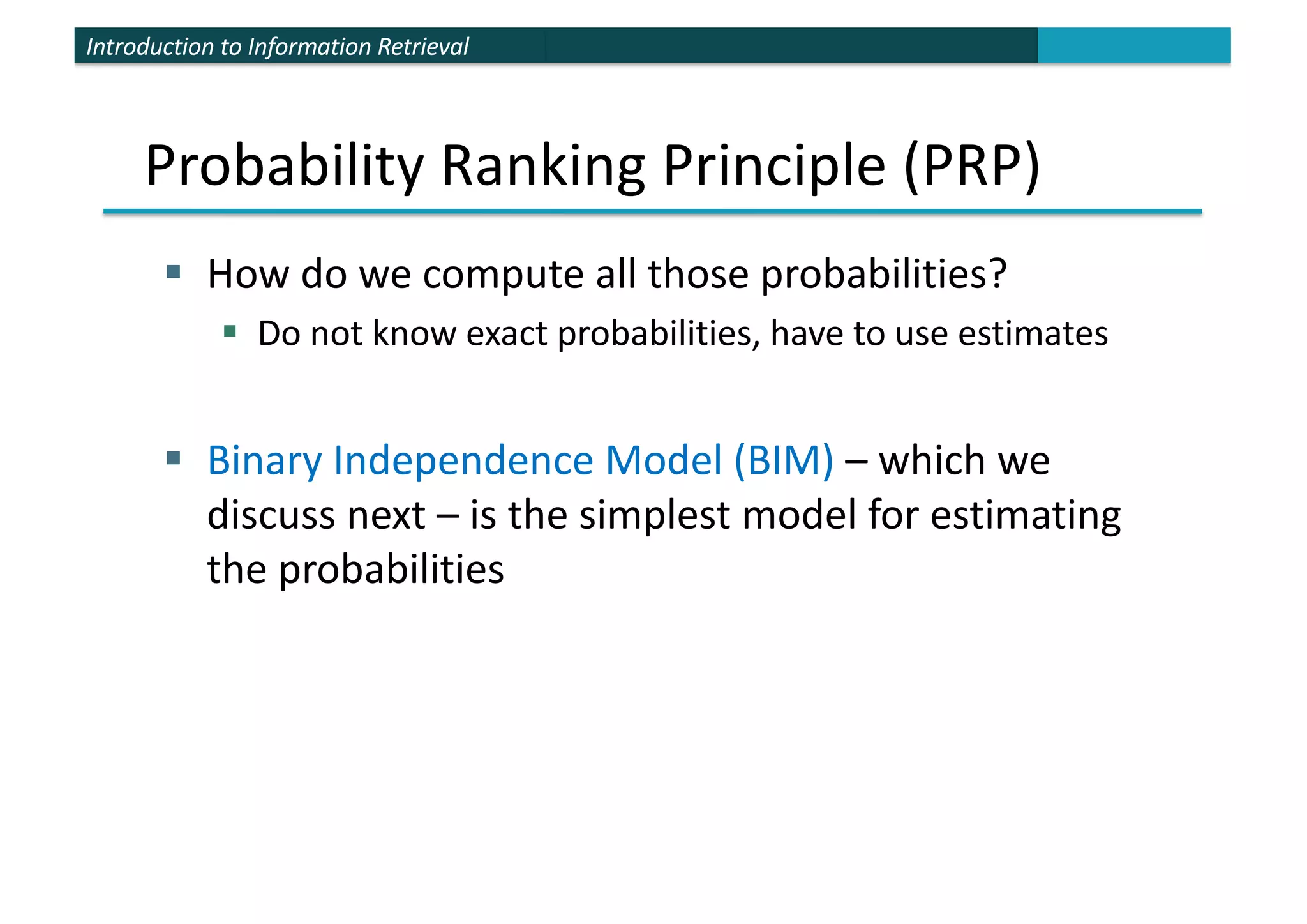
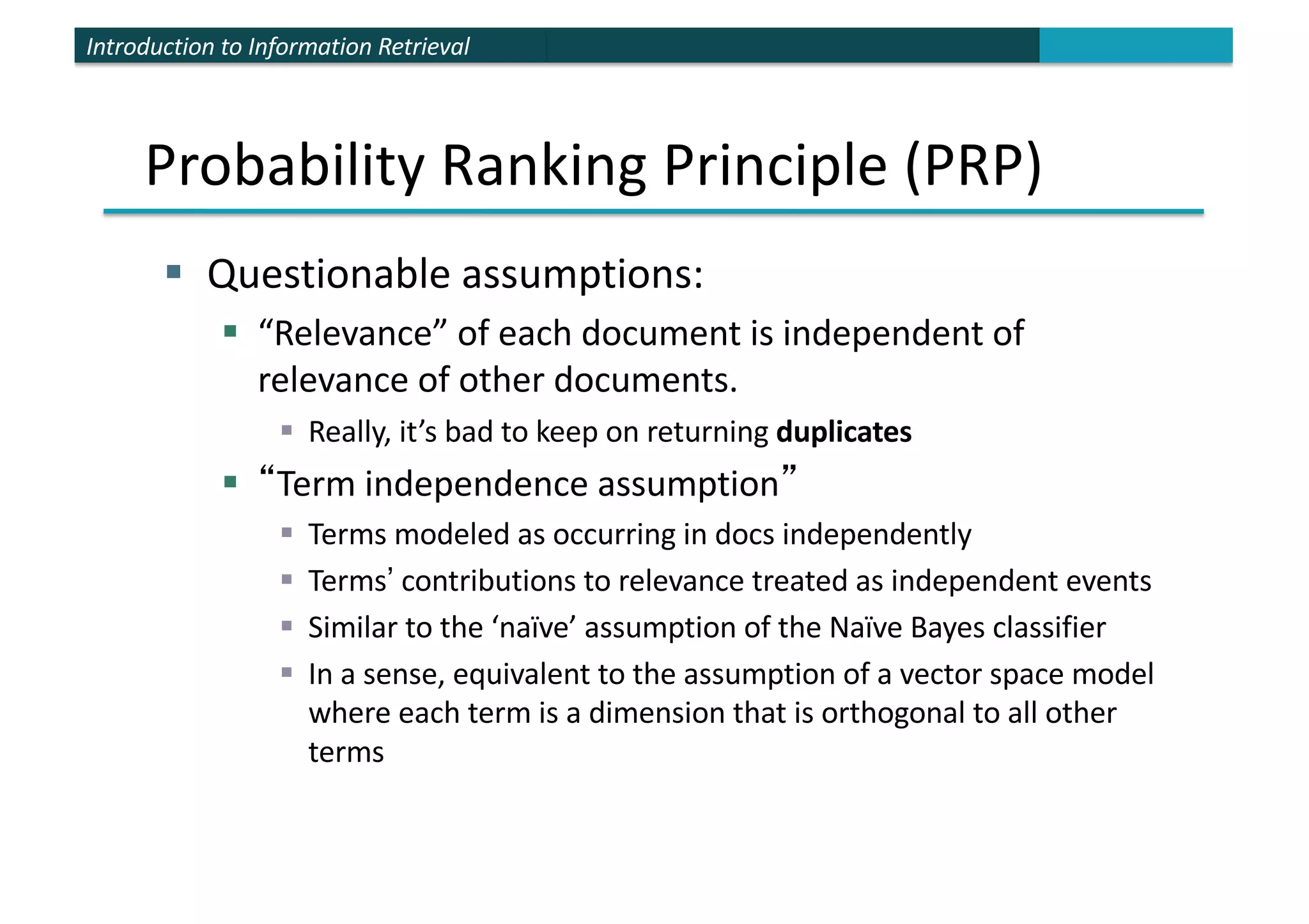
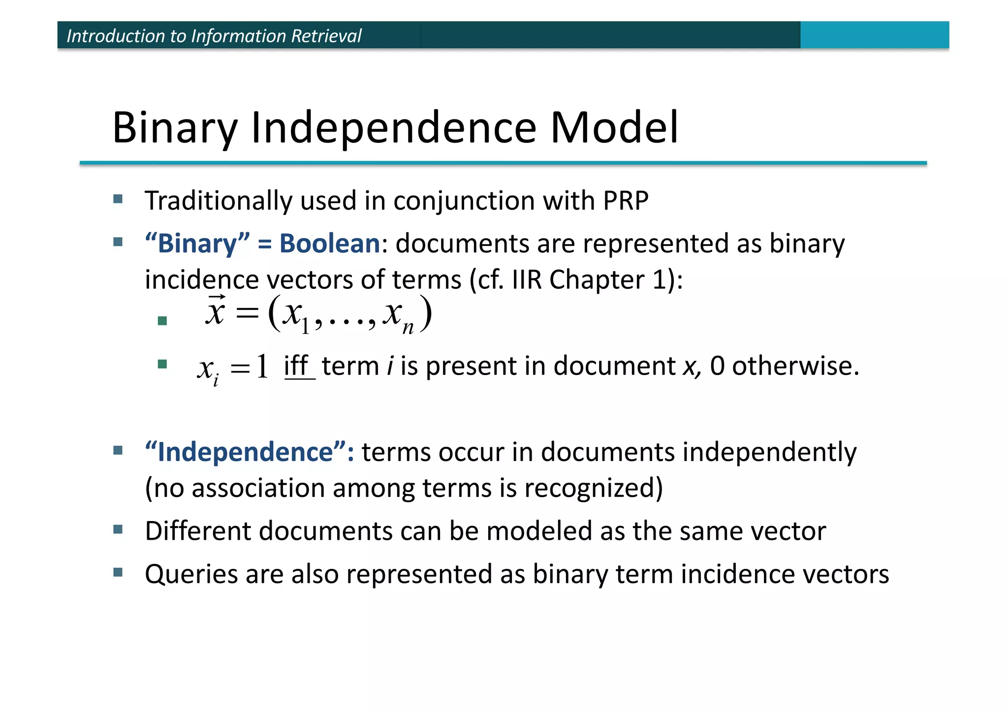
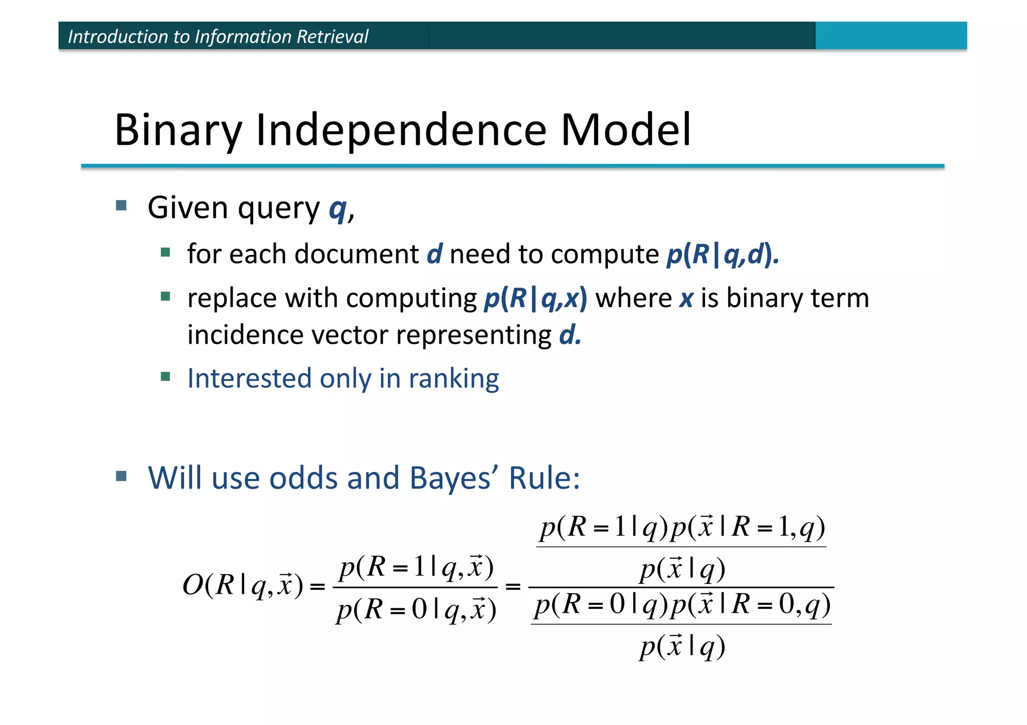
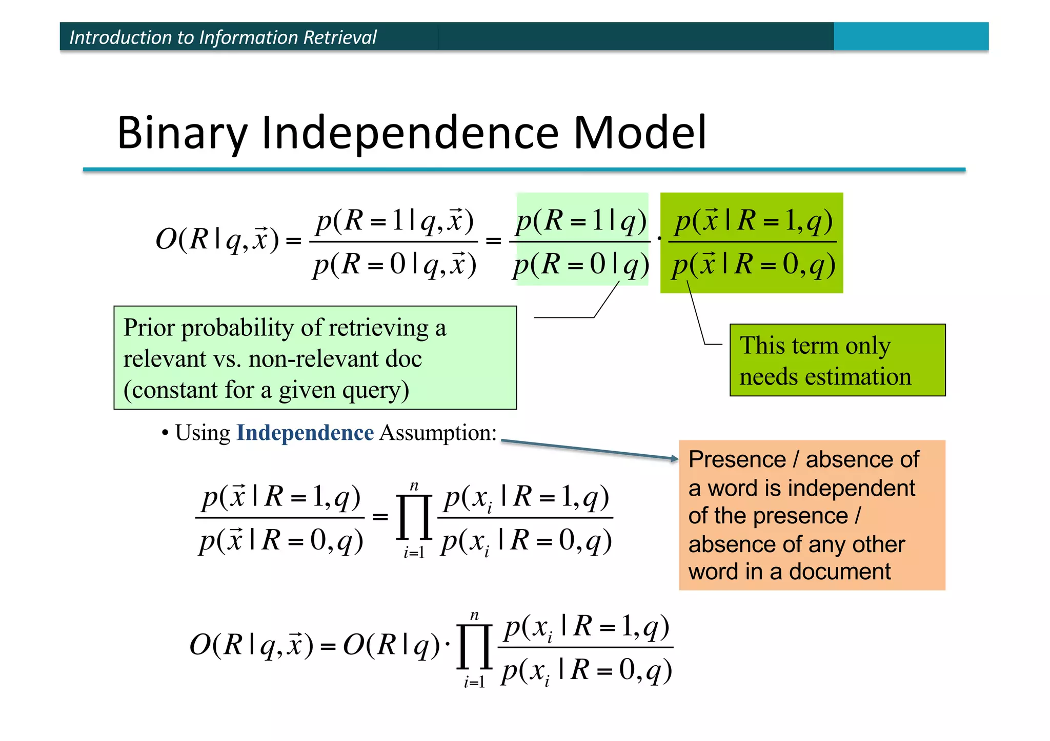
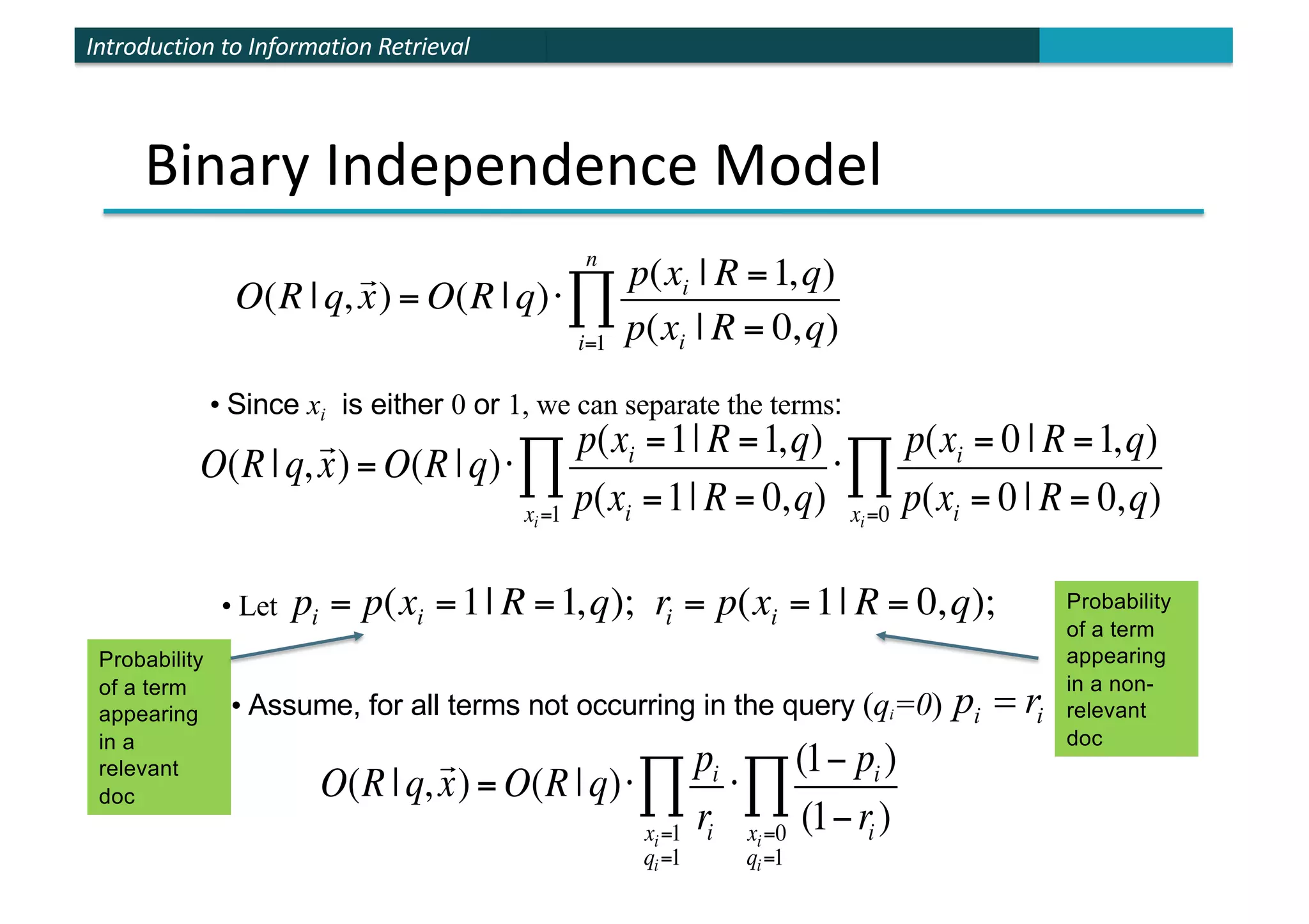
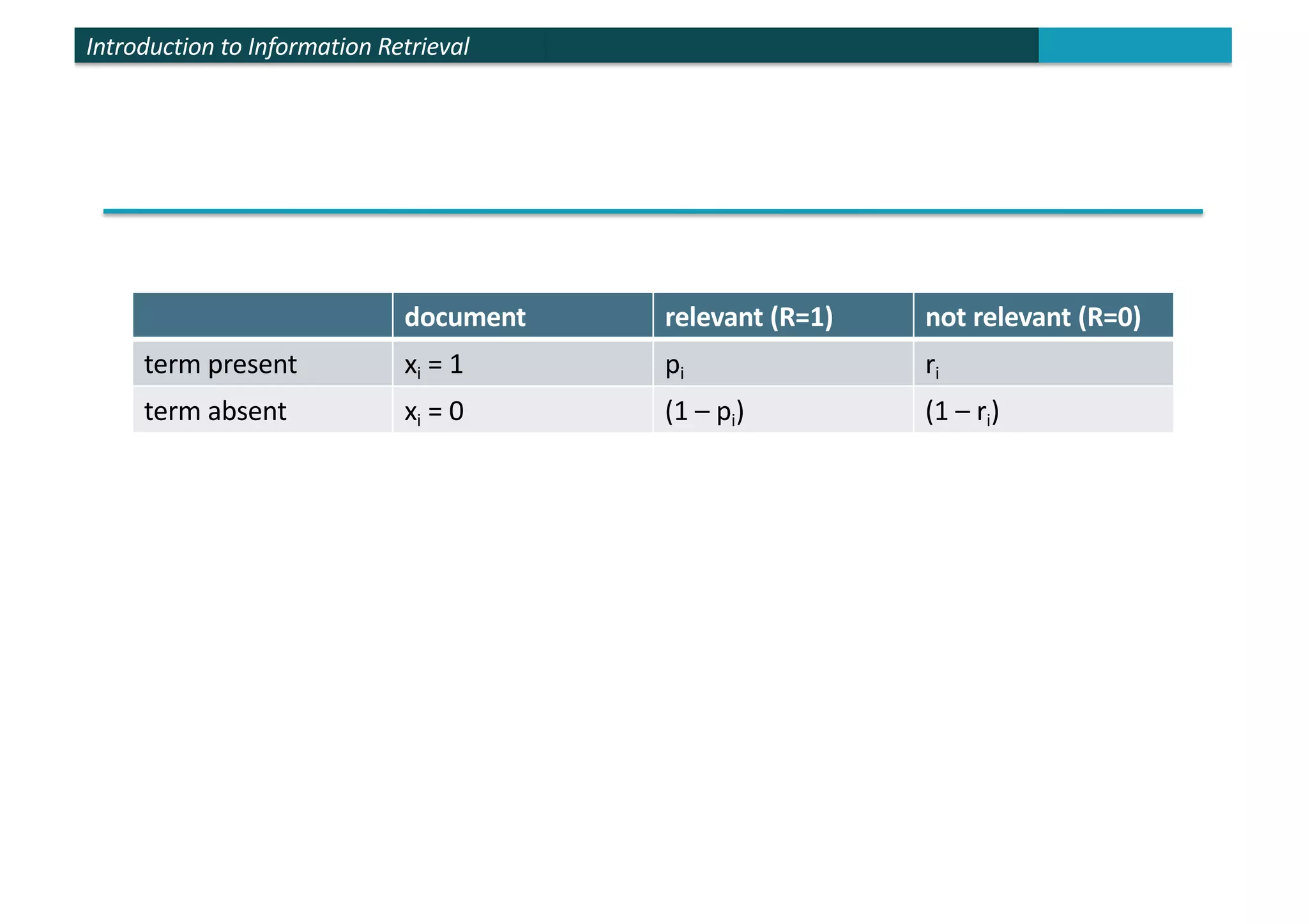
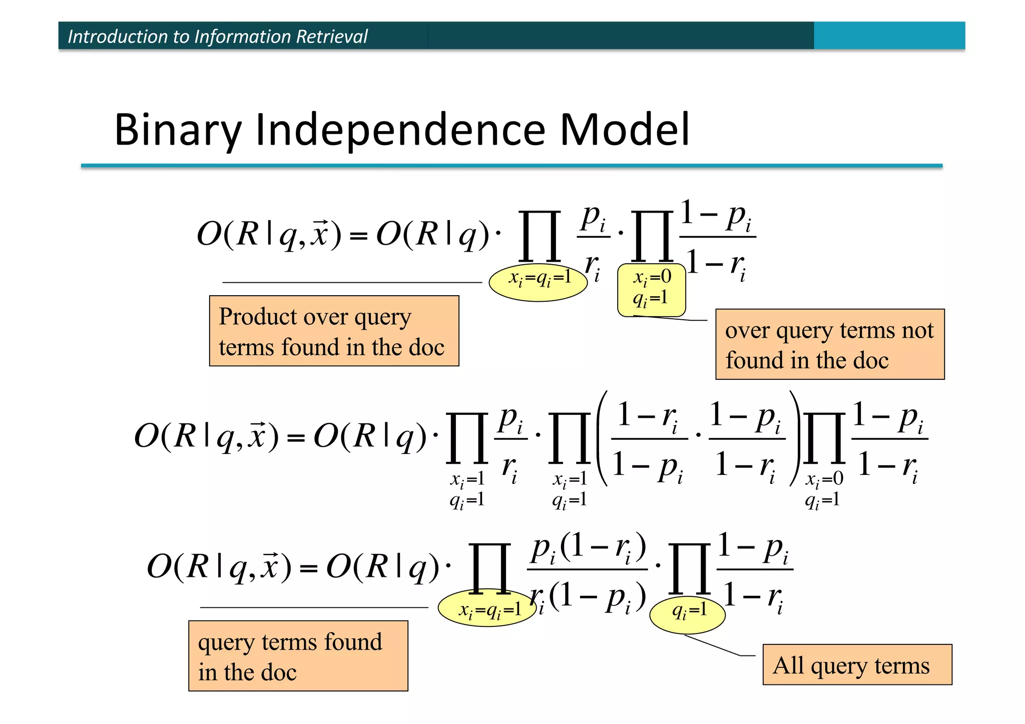
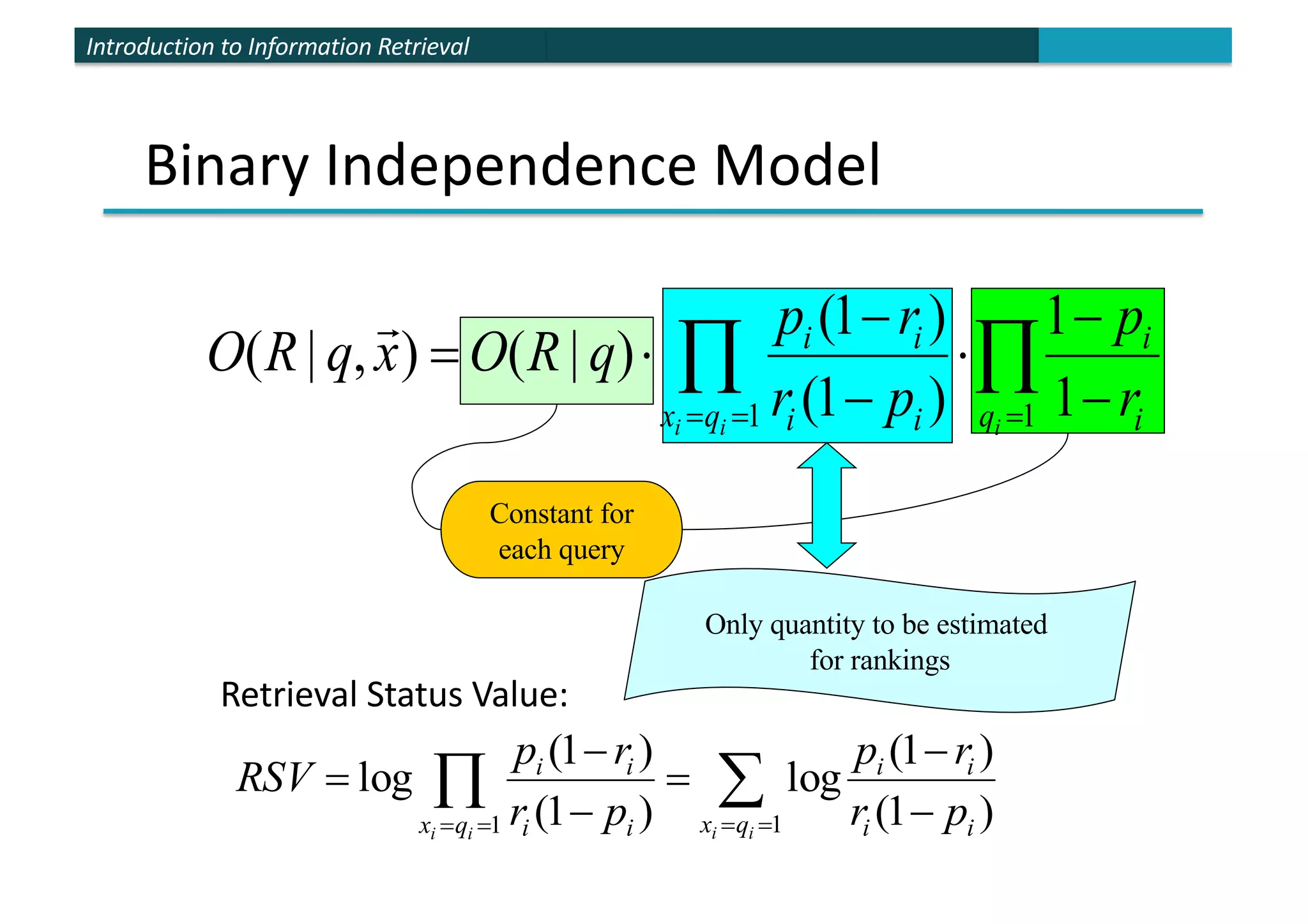
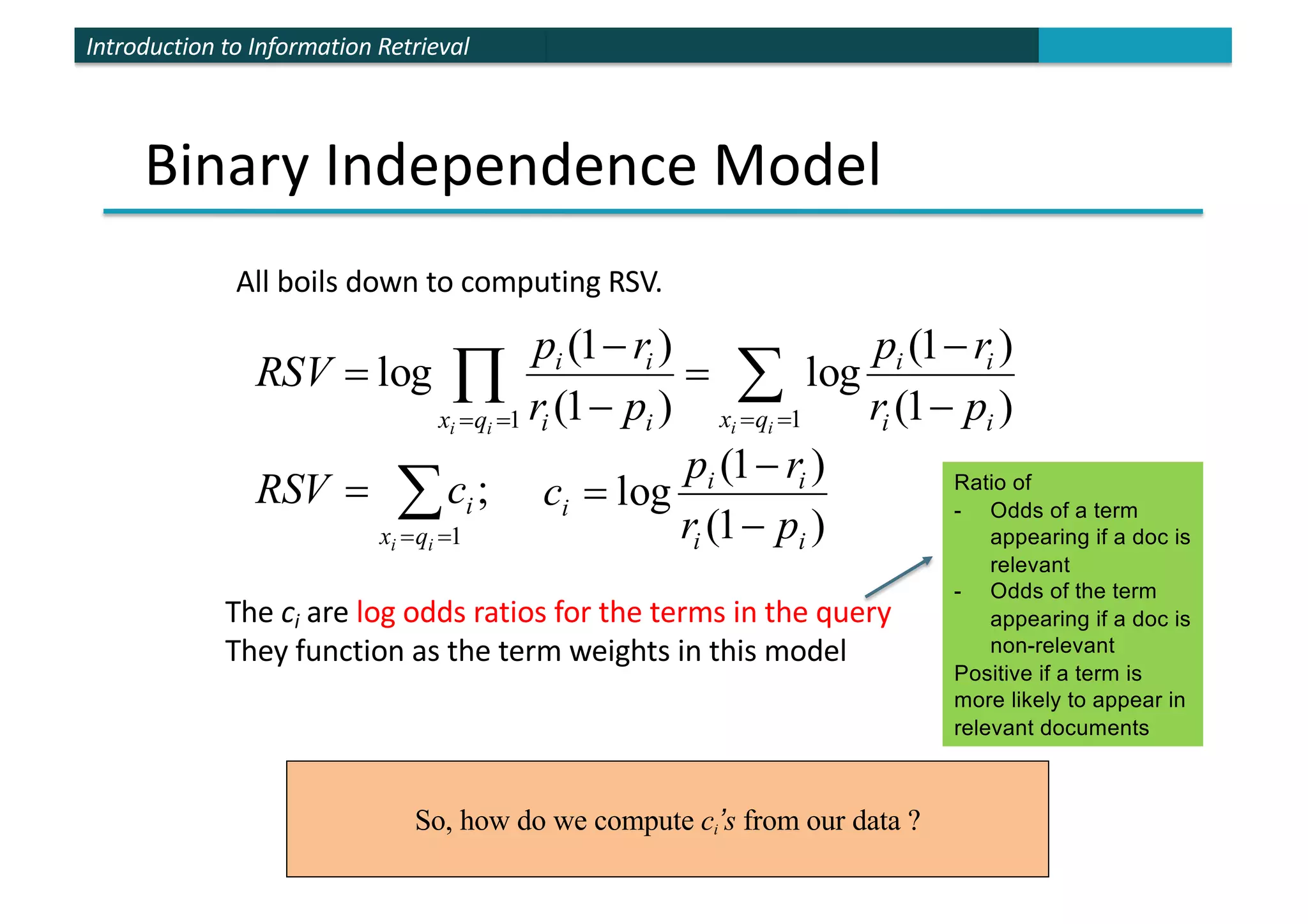
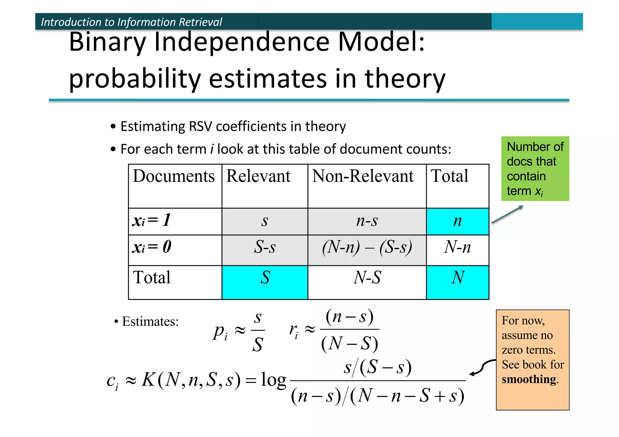
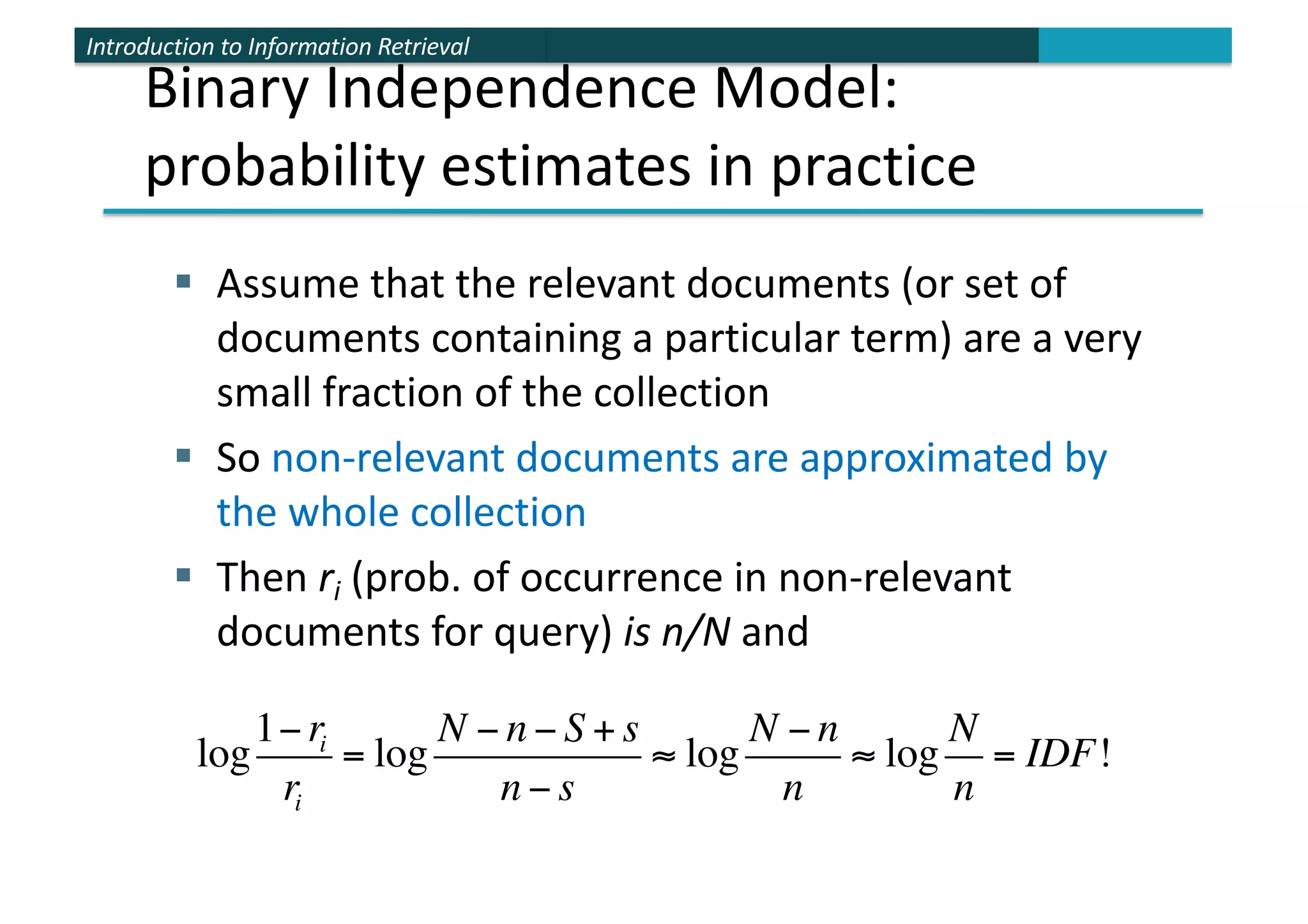
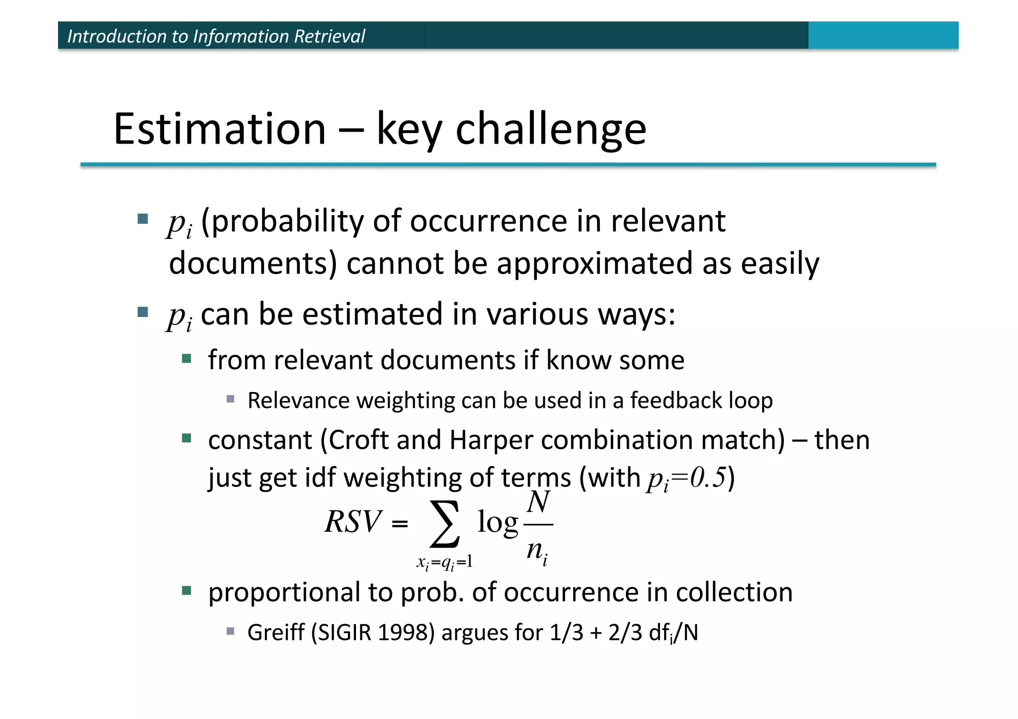
Introduction to Information Retrieval
Introduction to
Information Retrieval
Probabilistic Information Retrieval
Introduction to Information Retrieval
Why probabilities in IR?
User
Information Need
Documents
Document
Representation
Query
Representation
How to match?
Probabilities provide a principled foundation for uncertain reasoning.
Can we use probabilities to quantify our uncertainties?
Uncertain guess of
whether document
has relevant content
Understanding
of user need is
uncertain
Introduction to Information Retrieval
Probabilistic IR topics
§ Language model approach to IR
§ Classical probabilistic retrieval model
Introduction to Information Retrieval
The document ranking problem
§ We have a collection of documents
§ User issues a query
§ A list of documents needs to be returned
§ Ranking method is the core of an IR system:
§ In what order do we present documents to the user?
§ We want the “best” document to be first, second best
second, etc….
§ Idea: Rank by estimated probability of relevance of
the document w.r.t. information need
§ P(R=1|documenti, query)
Introduction to Information Retrieval
§ For events A and B:
§ Bayes’ Rule
§ Odds:
Prior
p(A, B) = p(A∩B) = p(A | B)p(B) = p(B | A)p(A)
p(A | B) =
p(B | A)p(A)
p(B)
=
p(B | A)p(A)
p(B | X)p(X)
X=A,A
∑
Recall a few probability basics
O(A) =
p(A)
p(A)
=
p(A)
1− p(A)
Posterior
Introduction to Information Retrieval
Probability Ranking Principle (PRP)
Let x represent a document in the collection.
Let R represent relevance of a document w.r.t. a given (fixed)
query and let R =1 represent relevant and R =0 not relevant.
p(R =1| x) =
p(x | R =1)p(R =1)
p(x)
p(R = 0 | x) =
p(x | R = 0)p(R = 0)
p(x)
p(x|R=1), p(x|R=0): probability that if a
relevant (not relevant) document is
retrieved, it is x.
Need to find p(R=1|x): probability that a document x is relevant;
Can rank documents in decreasing order of this probability.
p(R=1), p(R=0): prior probability
of retrieving a relevant or non-relevant
document
p(R = 0 | x)+ p(R =1| x) =1
Introduction to Information Retrieval
Probability Ranking Principle (PRP)
§ How do we compute all those probabilities?
§ Do not know exact probabilities, have to use estimates
§ Binary Independence Model (BIM) – which we
discuss next – is the simplest model for estimating
the probabilities
Introduction to Information Retrieval
Probability Ranking Principle (PRP)
§ Questionable assumptions:
§ “Relevance” of each document is independent of
relevance of other documents.
§ Really, it’s bad to keep on returning duplicates
§ “Term independence assumption”
§ Terms modeled as occurring in docs independently
§ Terms’ contributions to relevance treated as independent events
§ Similar to the ‘naïve’ assumption of the Naïve Bayes classifier
§ In a sense, equivalent to the assumption of a vector space model
where each term is a dimension that is orthogonal to all other
terms
Introduction to Information Retrieval
Probabilistic Ranking
Basic concept:
“For a given query, if we know some documents that are relevant, terms that
occur in those documents should be given greater weighting in searching for
other relevant documents.
By making assumptions about the distribution of terms and applying Bayes
Theorem, it is possible to derive weights theoretically.”
Van Rijsbergen
Introduction to Information Retrieval
Binary Independence Model
§ Traditionally used in conjunction with PRP
§ “Binary” = Boolean: documents are represented as binary
incidence vectors of terms (cf. IIR Chapter 1):
§
§ iff term i is present in document x, 0 otherwise.
§ “Independence”: terms occur in documents independently
(no association among terms is recognized)
§ Different documents can be modeled as the same vector
§ Queries are also represented as binary term incidence vectors
)
,
,
( 1 n
x
x
x !
"
=
1
=
i
x
Introduction to Information Retrieval
§ For events A and B:
§ Bayes’ Rule
§ Odds:
Prior
p(A, B) = p(A∩B) = p(A | B)p(B) = p(B | A)p(A)
p(A | B) =
p(B | A)p(A)
p(B)
=
p(B | A)p(A)
p(B | X)p(X)
X=A,A
∑
Recall a few probability basics
O(A) =
p(A)
p(A)
=
p(A)
1− p(A)
Posterior
Introduction to Information Retrieval
Binary Independence Model
§ Given query q,
§ for each document d need to compute p(R|q,d).
§ replace with computing p(R|q,x) where x is binary term
incidence vector representing d.
§ Interested only in ranking
§ Will use odds and Bayes’ Rule:
O(R | q,

x) =
p(R =1| q,

x)
p(R = 0 | q,

x)
=
p(R =1| q)p(

x | R =1,q)
p(

x | q)
p(R = 0 | q)p(

x | R = 0,q)
p(

x | q)
Introduction to Information Retrieval
Binary Independence Model
• Using Independence Assumption:
O(R | q,

x) = O(R | q)⋅
p(xi | R =1,q)
p(xi | R = 0,q)
i=1
n
∏
p(

x | R =1,q)
p(

x | R = 0,q)
=
p(xi | R =1,q)
p(xi | R = 0,q)
i=1
n
∏
O(R | q,

x) =
p(R =1| q,

x)
p(R = 0 | q,

x)
=
p(R =1| q)
p(R = 0 | q)
⋅
p(

x | R =1,q)
p(

x | R = 0,q)
Prior probability of retrieving a
relevant vs. non-relevant doc
(constant for a given query)
This term only
needs estimation
Presence / absence of
a word is independent
of the presence /
absence of any other
word in a document
Introduction to Information Retrieval
Binary Independence Model
• Since xi is either 0 or 1, we can separate the terms:
O(R |q,

x) = O(R |q)⋅
p(xi =1| R =1,q)
p(xi =1| R = 0,q)
xi=1
∏ ⋅
p(xi = 0 | R =1,q)
p(xi = 0 | R = 0,q)
xi=0
∏
• Let pi = p(xi =1| R =1,q); ri = p(xi =1| R = 0,q);
• Assume, for all terms not occurring in the query (qi=0) i
i r
p =
O(R | q,

x) = O(R | q)⋅
p(xi | R =1,q)
p(xi | R = 0,q)
i=1
n
∏
O(R |q,

x) = O(R |q)⋅
pi
ri
xi=1
qi=1
∏ ⋅
(1− pi )
(1−ri )
xi=0
qi=1
∏
Probability
of a term
appearing
in a
relevant
doc
Probability
of a term
appearing
in a non-
relevant
doc
Introduction to Information Retrieval
document relevant (R=1) not relevant (R=0)
term present xi = 1 pi ri
term absent xi = 0 (1 – pi) (1 – ri)
Introduction to Information Retrieval
Product over query
terms found in the doc
over query terms not
found in the doc
Binary Independence Model
query terms found
in the doc All query terms
O(R | q,

x) = O(R | q)⋅
pi
ri
xi=1
qi=1
∏ ⋅
1− ri
1− pi
⋅
1− pi
1− ri
$
%
&
'
(
)
xi=1
qi=1
∏
1− pi
1− ri
xi=0
qi=1
∏
O(R | q,

x) = O(R | q)⋅
pi (1− ri )
ri (1− pi )
xi=qi=1
∏ ⋅
1− pi
1− ri
qi=1
∏
O(R | q,

x) = O(R | q)⋅
pi
ri
xi=qi=1
∏ ⋅
1− pi
1− ri
xi=0
qi=1
∏
Introduction to Information Retrieval
Binary Independence Model
Constant for
each query
Only quantity to be estimated
for rankings
Õ
Õ =
=
= -
-
×
-
-
×
=
1
1 1
1
)
1
(
)
1
(
)
|
(
)
,
|
(
i
i
i q i
i
q
x i
i
i
i
r
p
p
r
r
p
q
R
O
x
q
R
O
!
Retrieval Status Value:
å
Õ =
=
=
= -
-
=
-
-
=
1
1 )
1
(
)
1
(
log
)
1
(
)
1
(
log
i
i
i
i q
x i
i
i
i
q
x i
i
i
i
p
r
r
p
p
r
r
p
RSV
Introduction to Information Retrieval
Binary Independence Model
All boils down to computing RSV.
å
Õ =
=
=
= -
-
=
-
-
=
1
1 )
1
(
)
1
(
log
)
1
(
)
1
(
log
i
i
i
i q
x i
i
i
i
q
x i
i
i
i
p
r
r
p
p
r
r
p
RSV
å=
=
=
1
;
i
i q
x
i
c
RSV
)
1
(
)
1
(
log
i
i
i
i
i
p
r
r
p
c
-
-
=
So, how do we compute ci’s from our data ?
The ci are log odds ratios for the terms in the query
They function as the term weights in this model
Ratio of
- Odds of a term
appearing if a doc is
relevant
- Odds of the term
appearing if a doc is
non-relevant
Positive if a term is
more likely to appear in
relevant documents
Introduction to Information Retrieval
Binary Independence Model:
probability estimates in theory
• Estimating RSV coefficients in theory
• For each term i look at this table of document counts:
Documents Relevant Non-Relevant Total
xi = 1 s n-s n
xi = 0 S-s (N-n) – (S-s) N-n
Total S N-S N
S
s
pi »
)
(
)
(
S
N
s
n
ri
-
-
»
)
(
)
(
)
(
log
)
,
,
,
(
s
S
n
N
s
n
s
S
s
s
S
n
N
K
ci
+
-
-
-
-
=
»
• Estimates: For now,
assume no
zero terms.
See book for
smoothing.
Number of
docs that
contain
term xi
Introduction to Information Retrieval
§ Assume that the relevant documents (or set of
documents containing a particular term) are a very
small fraction of the collection
§ So non-relevant documents are approximated by
the whole collection
§ Then ri (prob. of occurrence in non-relevant
documents for query) is n/N and
log
1−ri
ri
= log
N − n − S + s
n − s
≈ log
N − n
n
≈ log
N
n
= IDF!
Binary Independence Model:
probability estimates in practice
Introduction to Information Retrieval
Estimation – key challenge
§ pi (probability of occurrence in relevant
documents) cannot be approximated as easily
§ pi can be estimated in various ways:
§ from relevant documents if know some
§ Relevance weighting can be used in a feedback loop
§ constant (Croft and Harper combination match) – then
just get idf weighting of terms (with pi=0.5)
§ proportional to prob. of occurrence in collection
§ Greiff (SIGIR 1998) argues for 1/3 + 2/3 dfi/N
RSV = log
N
ni
xi=qi=1
∑
Introduction to Information Retrieval
Okapi BM25: A non-binary model
Introduction to Information Retrieval
Okapi BM25: A Non-binary Model
• The Binary Independence Model (BIM) was originally
designed for short catalog records of fairly consistent length,
and it works reasonably in these contexts
• For modern full-text search collections, a model should pay
attention to term frequency and document length
• BestMatch25 (a.k.a BM25 or Okapi) is designed to be
sensitive to these quantities
• From 1994 until today, BM25 is one of the most widely used
and robust retrieval models
23
Introduction to Information Retrieval
Okapi BM25: A Non-binary Model
§The simplest score for document d is just idf weighting of the query
terms present in the document:
§Improve this formula by factoring in the term frequency and document
length:
§ tf td : term frequency in document d
§ Ld (Lave): length of document d (average document length in the whole
collection)
§ k1: tuning parameter controlling the document term frequency scaling
(0 means no TF, i.e., Binary model; large value means use raw TF)
§ b: tuning parameter controlling the scaling by document length (0
means no length normalization)
24
Introduction to Information Retrieval
Saturation function
§ For high values of k1, increments in tfi continue to
contribute significantly to the score
§ Contributions tail off quickly for low values of k1
Introduction to Information Retrieval
Okapi BM25: A Non-binary Model
§If the query is long, we might also use similar weighting for query
terms
§ tf tq: term frequency in the query q
§k3: tuning parameter controlling term frequency scaling of the query
§ No length normalisation of queries (because retrieval is being done
with respect to a single fixed query)
§ The above tuning parameters should ideally be set to optimize
performance on a development test collection. In the absence of
such optimisation, experiments have shown reasonable values are to
set k1 and k3 to a value between 1.2 and 2 and b = 0.75
26

IR-lec17-probabilistic-ir.pdf

  • 1.
    Introduction to InformationRetrieval Introduction to Information Retrieval Probabilistic Information Retrieval
  • 2.
    Introduction to InformationRetrieval Why probabilities in IR? User Information Need Documents Document Representation Query Representation How to match? Probabilities provide a principled foundation for uncertain reasoning. Can we use probabilities to quantify our uncertainties? Uncertain guess of whether document has relevant content Understanding of user need is uncertain
  • 3.
    Introduction to InformationRetrieval Probabilistic IR topics § Language model approach to IR § Classical probabilistic retrieval model
  • 4.
    Introduction to InformationRetrieval The document ranking problem § We have a collection of documents § User issues a query § A list of documents needs to be returned § Ranking method is the core of an IR system: § In what order do we present documents to the user? § We want the “best” document to be first, second best second, etc…. § Idea: Rank by estimated probability of relevance of the document w.r.t. information need § P(R=1|documenti, query)
  • 5.
    Introduction to InformationRetrieval § For events A and B: § Bayes’ Rule § Odds: Prior p(A, B) = p(A∩B) = p(A | B)p(B) = p(B | A)p(A) p(A | B) = p(B | A)p(A) p(B) = p(B | A)p(A) p(B | X)p(X) X=A,A ∑ Recall a few probability basics O(A) = p(A) p(A) = p(A) 1− p(A) Posterior
  • 6.
    Introduction to InformationRetrieval Probability Ranking Principle (PRP) Let x represent a document in the collection. Let R represent relevance of a document w.r.t. a given (fixed) query and let R =1 represent relevant and R =0 not relevant. p(R =1| x) = p(x | R =1)p(R =1) p(x) p(R = 0 | x) = p(x | R = 0)p(R = 0) p(x) p(x|R=1), p(x|R=0): probability that if a relevant (not relevant) document is retrieved, it is x. Need to find p(R=1|x): probability that a document x is relevant; Can rank documents in decreasing order of this probability. p(R=1), p(R=0): prior probability of retrieving a relevant or non-relevant document p(R = 0 | x)+ p(R =1| x) =1
  • 7.
    Introduction to InformationRetrieval Probability Ranking Principle (PRP) § How do we compute all those probabilities? § Do not know exact probabilities, have to use estimates § Binary Independence Model (BIM) – which we discuss next – is the simplest model for estimating the probabilities
  • 8.
    Introduction to InformationRetrieval Probability Ranking Principle (PRP) § Questionable assumptions: § “Relevance” of each document is independent of relevance of other documents. § Really, it’s bad to keep on returning duplicates § “Term independence assumption” § Terms modeled as occurring in docs independently § Terms’ contributions to relevance treated as independent events § Similar to the ‘naïve’ assumption of the Naïve Bayes classifier § In a sense, equivalent to the assumption of a vector space model where each term is a dimension that is orthogonal to all other terms
  • 9.
    Introduction to InformationRetrieval Probabilistic Ranking Basic concept: “For a given query, if we know some documents that are relevant, terms that occur in those documents should be given greater weighting in searching for other relevant documents. By making assumptions about the distribution of terms and applying Bayes Theorem, it is possible to derive weights theoretically.” Van Rijsbergen
  • 10.
    Introduction to InformationRetrieval Binary Independence Model § Traditionally used in conjunction with PRP § “Binary” = Boolean: documents are represented as binary incidence vectors of terms (cf. IIR Chapter 1): § § iff term i is present in document x, 0 otherwise. § “Independence”: terms occur in documents independently (no association among terms is recognized) § Different documents can be modeled as the same vector § Queries are also represented as binary term incidence vectors ) , , ( 1 n x x x ! " = 1 = i x
  • 11.
    Introduction to InformationRetrieval § For events A and B: § Bayes’ Rule § Odds: Prior p(A, B) = p(A∩B) = p(A | B)p(B) = p(B | A)p(A) p(A | B) = p(B | A)p(A) p(B) = p(B | A)p(A) p(B | X)p(X) X=A,A ∑ Recall a few probability basics O(A) = p(A) p(A) = p(A) 1− p(A) Posterior
  • 12.
    Introduction to InformationRetrieval Binary Independence Model § Given query q, § for each document d need to compute p(R|q,d). § replace with computing p(R|q,x) where x is binary term incidence vector representing d. § Interested only in ranking § Will use odds and Bayes’ Rule: O(R | q,  x) = p(R =1| q,  x) p(R = 0 | q,  x) = p(R =1| q)p(  x | R =1,q) p(  x | q) p(R = 0 | q)p(  x | R = 0,q) p(  x | q)
  • 13.
    Introduction to InformationRetrieval Binary Independence Model • Using Independence Assumption: O(R | q,  x) = O(R | q)⋅ p(xi | R =1,q) p(xi | R = 0,q) i=1 n ∏ p(  x | R =1,q) p(  x | R = 0,q) = p(xi | R =1,q) p(xi | R = 0,q) i=1 n ∏ O(R | q,  x) = p(R =1| q,  x) p(R = 0 | q,  x) = p(R =1| q) p(R = 0 | q) ⋅ p(  x | R =1,q) p(  x | R = 0,q) Prior probability of retrieving a relevant vs. non-relevant doc (constant for a given query) This term only needs estimation Presence / absence of a word is independent of the presence / absence of any other word in a document
  • 14.
    Introduction to InformationRetrieval Binary Independence Model • Since xi is either 0 or 1, we can separate the terms: O(R |q,  x) = O(R |q)⋅ p(xi =1| R =1,q) p(xi =1| R = 0,q) xi=1 ∏ ⋅ p(xi = 0 | R =1,q) p(xi = 0 | R = 0,q) xi=0 ∏ • Let pi = p(xi =1| R =1,q); ri = p(xi =1| R = 0,q); • Assume, for all terms not occurring in the query (qi=0) i i r p = O(R | q,  x) = O(R | q)⋅ p(xi | R =1,q) p(xi | R = 0,q) i=1 n ∏ O(R |q,  x) = O(R |q)⋅ pi ri xi=1 qi=1 ∏ ⋅ (1− pi ) (1−ri ) xi=0 qi=1 ∏ Probability of a term appearing in a relevant doc Probability of a term appearing in a non- relevant doc
  • 15.
    Introduction to InformationRetrieval document relevant (R=1) not relevant (R=0) term present xi = 1 pi ri term absent xi = 0 (1 – pi) (1 – ri)
  • 16.
    Introduction to InformationRetrieval Product over query terms found in the doc over query terms not found in the doc Binary Independence Model query terms found in the doc All query terms O(R | q,  x) = O(R | q)⋅ pi ri xi=1 qi=1 ∏ ⋅ 1− ri 1− pi ⋅ 1− pi 1− ri $ % & ' ( ) xi=1 qi=1 ∏ 1− pi 1− ri xi=0 qi=1 ∏ O(R | q,  x) = O(R | q)⋅ pi (1− ri ) ri (1− pi ) xi=qi=1 ∏ ⋅ 1− pi 1− ri qi=1 ∏ O(R | q,  x) = O(R | q)⋅ pi ri xi=qi=1 ∏ ⋅ 1− pi 1− ri xi=0 qi=1 ∏
  • 17.
    Introduction to InformationRetrieval Binary Independence Model Constant for each query Only quantity to be estimated for rankings Õ Õ = = = - - × - - × = 1 1 1 1 ) 1 ( ) 1 ( ) | ( ) , | ( i i i q i i q x i i i i r p p r r p q R O x q R O ! Retrieval Status Value: å Õ = = = = - - = - - = 1 1 ) 1 ( ) 1 ( log ) 1 ( ) 1 ( log i i i i q x i i i i q x i i i i p r r p p r r p RSV
  • 18.
    Introduction to InformationRetrieval Binary Independence Model All boils down to computing RSV. å Õ = = = = - - = - - = 1 1 ) 1 ( ) 1 ( log ) 1 ( ) 1 ( log i i i i q x i i i i q x i i i i p r r p p r r p RSV å= = = 1 ; i i q x i c RSV ) 1 ( ) 1 ( log i i i i i p r r p c - - = So, how do we compute ci’s from our data ? The ci are log odds ratios for the terms in the query They function as the term weights in this model Ratio of - Odds of a term appearing if a doc is relevant - Odds of the term appearing if a doc is non-relevant Positive if a term is more likely to appear in relevant documents
  • 19.
    Introduction to InformationRetrieval Binary Independence Model: probability estimates in theory • Estimating RSV coefficients in theory • For each term i look at this table of document counts: Documents Relevant Non-Relevant Total xi = 1 s n-s n xi = 0 S-s (N-n) – (S-s) N-n Total S N-S N S s pi » ) ( ) ( S N s n ri - - » ) ( ) ( ) ( log ) , , , ( s S n N s n s S s s S n N K ci + - - - - = » • Estimates: For now, assume no zero terms. See book for smoothing. Number of docs that contain term xi
  • 20.
    Introduction to InformationRetrieval § Assume that the relevant documents (or set of documents containing a particular term) are a very small fraction of the collection § So non-relevant documents are approximated by the whole collection § Then ri (prob. of occurrence in non-relevant documents for query) is n/N and log 1−ri ri = log N − n − S + s n − s ≈ log N − n n ≈ log N n = IDF! Binary Independence Model: probability estimates in practice
  • 21.
    Introduction to InformationRetrieval Estimation – key challenge § pi (probability of occurrence in relevant documents) cannot be approximated as easily § pi can be estimated in various ways: § from relevant documents if know some § Relevance weighting can be used in a feedback loop § constant (Croft and Harper combination match) – then just get idf weighting of terms (with pi=0.5) § proportional to prob. of occurrence in collection § Greiff (SIGIR 1998) argues for 1/3 + 2/3 dfi/N RSV = log N ni xi=qi=1 ∑
  • 22.
    Introduction to InformationRetrieval Okapi BM25: A non-binary model
  • 23.
    Introduction to InformationRetrieval Okapi BM25: A Non-binary Model • The Binary Independence Model (BIM) was originally designed for short catalog records of fairly consistent length, and it works reasonably in these contexts • For modern full-text search collections, a model should pay attention to term frequency and document length • BestMatch25 (a.k.a BM25 or Okapi) is designed to be sensitive to these quantities • From 1994 until today, BM25 is one of the most widely used and robust retrieval models 23
  • 24.
    Introduction to InformationRetrieval Okapi BM25: A Non-binary Model §The simplest score for document d is just idf weighting of the query terms present in the document: §Improve this formula by factoring in the term frequency and document length: § tf td : term frequency in document d § Ld (Lave): length of document d (average document length in the whole collection) § k1: tuning parameter controlling the document term frequency scaling (0 means no TF, i.e., Binary model; large value means use raw TF) § b: tuning parameter controlling the scaling by document length (0 means no length normalization) 24
  • 25.
    Introduction to InformationRetrieval Saturation function § For high values of k1, increments in tfi continue to contribute significantly to the score § Contributions tail off quickly for low values of k1
  • 26.
    Introduction to InformationRetrieval Okapi BM25: A Non-binary Model §If the query is long, we might also use similar weighting for query terms § tf tq: term frequency in the query q §k3: tuning parameter controlling term frequency scaling of the query § No length normalisation of queries (because retrieval is being done with respect to a single fixed query) § The above tuning parameters should ideally be set to optimize performance on a development test collection. In the absence of such optimisation, experiments have shown reasonable values are to set k1 and k3 to a value between 1.2 and 2 and b = 0.75 26