This document provides an introduction to a textbook on software testing. It describes the textbook's approach of defining testing as applying well-defined test criteria to a model of the software. The textbook covers various coverage criteria for testing source code, designs, specifications, use cases, and other software artifacts. It also describes the authors' credentials and the supplementary materials available on the textbook's website.


![introtest CUUS047-Ammann ISBN 9780521880381 November 8, 2007 17:13 Char Count= 0
8 Overview
The Pentium bug not only illustrates the difference in testing levels, but it is also
one of the best arguments for paying more attention to unit testing. There are no
shortcuts – all aspects of software need to be tested.
On the other hand, some faults can only be found at the system level. One dra-
matic example was the launch failure of the first Ariane 5 rocket, which exploded
37 seconds after liftoff on June 4, 1996. The low-level cause was an unhandled
floating-point conversion exception in an internal guidance system function. It
turned out that the guidance system could never encounter the unhandled exception
when used on the Ariane 4 rocket. In other words, the guidance system function is
correct for Ariane 4. The developers of the Ariane 5 quite reasonably wanted to
reuse the successful inertial guidance system from the Ariane 4, but no one reana-
lyzed the software in light of the substantially different flight trajectory of Ariane 5.
Furthermore, the system tests that would have found the problem were technically
difficult to execute, and so were not performed. The result was spectacular – and
expensive!
Another public failure was the Mars lander of September 1999, which crashed
due to a misunderstanding in the units of measure used by two modules created by
separate software groups. One module computed thruster data in English units and
forwarded the data to a module that expected data in metric units. This is a very
typical integration fault (but in this case enormously expensive, both in terms of
money and prestige).
One final note is that object-oriented (OO) software changes the testing levels.
OO software blurs the distinction between units and modules, so the OO software
testing literature has developed a slight variation of these levels. Intramethod testing
is when tests are constructed for individual methods. Intermethod testing is when
pairs of methods within the same class are tested in concert. Intraclass testing is
when tests are constructed for a single entire class, usually as sequences of calls to
methods within the class. Finally, interclass testing is when more than one class is
tested at the same time. The first three are variations of unit and module testing,
whereas interclass testing is a type of integration testing.
1.1.2 Beizer’s Testing Levels Based on Test Process Maturity
Another categorization of levels is based on the test process maturity level of an
organization. Each level is characterized by the goal of the test engineers. The fol-
lowing material is adapted from Beizer [29].
Level 0 There’s no difference between testing and debugging.
Level 1 The purpose of testing is to show that the software works.
Level 2 The purpose of testing is to show that the software doesn’t work.
Level 3 The purpose of testing is not to prove anything specific, but to reduce
the risk of using the software.
Level 4 Testing is a mental discipline that helps all IT professionals develop
higher quality software.
Level 0 is the view that testing is the same as debugging. This is the view that
is naturally adopted by many undergraduate computer science majors. In most CS
programming classes, the students get their programs to compile, then debug the
programs with a few inputs chosen either arbitrarily or provided by the professor.](https://image.slidesharecdn.com/introductiontosoftwaretesting-221201191322-f16668ac/85/Introduction-to-Software-Testing-pdf-32-320.jpg)
![introtest CUUS047-Ammann ISBN 9780521880381 November 8, 2007 17:13 Char Count= 0
12 Overview
development. This can sometimes mean that validation is given more weight than
verification.
Two terms that we have already used are fault and failure. Understanding this dis-
tinction is the first step in moving from level 0 thinking to level 1 thinking. We adopt
the definition of software fault, error, and failure from the dependability community.
Definition 1.3 Software Fault: A static defect in the software.
Definition 1.4 Software Error: An incorrect internal state that is the manifes-
tation of some fault.
Definition 1.5 Software Failure: External, incorrect behavior with respect to
the requirements or other description of the expected behavior.
Consider a medical doctor making a diagnosis for a patient. The patient enters
the doctor’s office with a list of failures (that is, symptoms). The doctor then must
discover the fault, or root cause of the symptom. To aid in the diagnosis, a doctor
may order tests that look for anomalous internal conditions, such as high blood
pressure, an irregular heartbeat, high levels of blood glucose, or high cholesterol. In
our terminology, these anomalous internal conditions correspond to errors.
While this analogy may help the student clarify his or her thinking about faults,
errors, and failures, software testing and a doctor’s diagnosis differ in one crucial
way. Specifically, faults in software are design mistakes. They do not appear spon-
taneously, but rather exist as a result of some (unfortunate) decision by a human.
Medical problems (as well as faults in computer system hardware), on the other
hand, are often a result of physical degradation. This distinction is important be-
cause it explains the limits on the extent to which any process can hope to control
software faults. Specifically, since no foolproof way exists to catch arbitrary mis-
takes made by humans, we cannot eliminate all faults from software. In colloquial
terms, we can make software development foolproof, but we cannot, and should not
attempt to, make it damn-foolproof.
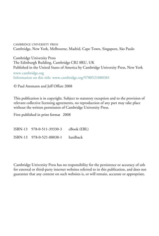
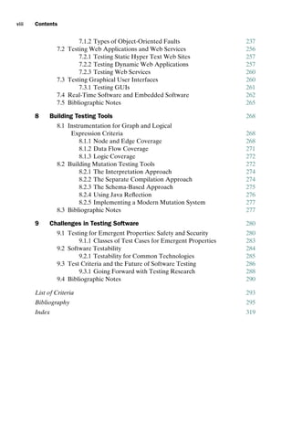
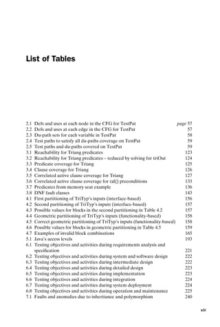
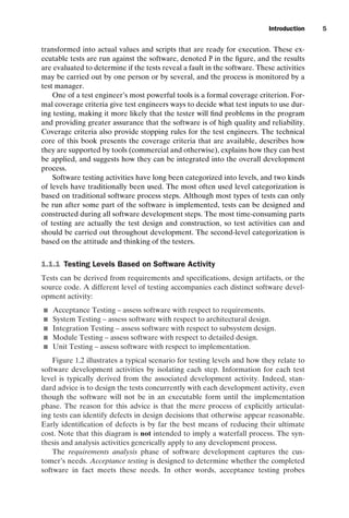
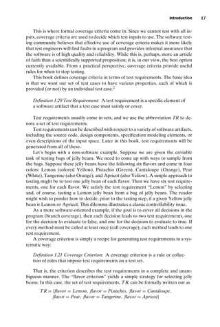
For a more technical example of the definitions of fault, error, and failure, con-
sider the following Java method:
public static int numZero (int[] x) {
// Effects: if x == null throw NullPointerException
// else return the number of occurrences of 0 in x
int count = 0;
for (int i = 1; i x.length; i++)
{
if (x[i] == 0)
{
count++;
}
}
return count;
}](https://image.slidesharecdn.com/introductiontosoftwaretesting-221201191322-f16668ac/85/Introduction-to-Software-Testing-pdf-36-320.jpg)
![introtest CUUS047-Ammann ISBN 9780521880381 November 8, 2007 17:13 Char Count= 0
Introduction 13
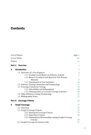
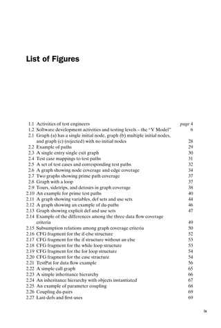
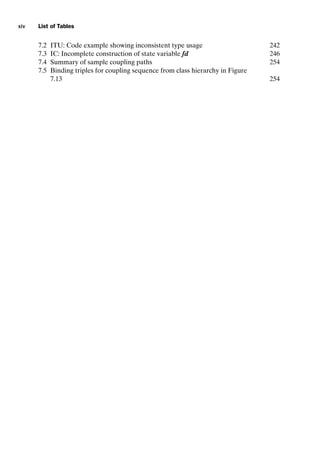
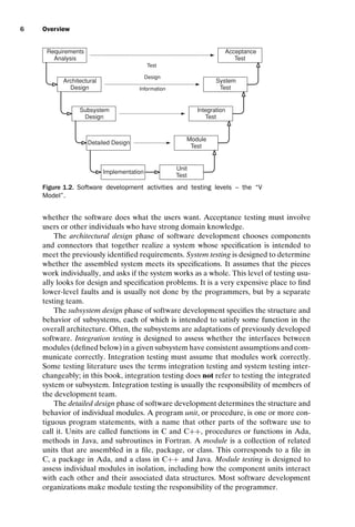
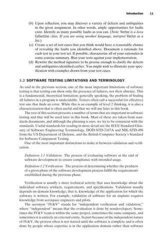
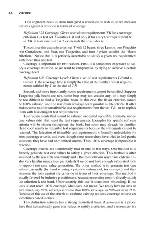
The fault in this program is that it starts looking for zeroes at index 1 instead
of index 0, as is necessary for arrays in Java. For example, numZero ([2, 7, 0]) cor-
rectly evaluates to 1, while numZero ([0, 7, 2]) incorrectly evaluates to 0. In both
of these cases the fault is executed. Although both of these cases result in an error,
only the second case results in failure. To understand the error states, we need to
identify the state for the program. The state for numZero consists of values for the
variables x, count, i, and the program counter (denoted PC). For the first example
given above, the state at the if statement on the very first iteration of the loop is
( x = [2, 7, 0], count = 0, i = 1, PC = if). Notice that this state is in error precisely be-
cause the value of i should be zero on the first iteration. However, since the value of
count is coincidentally correct, the error state does not propagate to the output, and
hence the software does not fail. In other words, a state is in error simply if it is not
the expected state, even if all of the values in the state, considered in isolation, are
acceptable. More generally, if the required sequence of states is s0, s1, s2, . . . , and
the actual sequence of states is s0, s2, s3, . . . , then state s2 is in error in the second
sequence.
In the second case the corresponding (error) state is (x = [0, 7, 2], count = 0, i =
1, PC = if). In this case, the error propagates to the variable count and is present in
the return value of the method. Hence a failure results.
The definitions of fault and failure allow us to distinguish testing from debugg-
ing.
Definition 1.6 Testing: Evaluating software by observing its execution.
Definition 1.7 Test Failure: Execution that results in a failure.
Definition 1.8 Debugging: The process of finding a fault given a failure.
Of course the central issue is that for a given fault, not all inputs will “trigger”
the fault into creating incorrect output (a failure). Also, it is often very difficult to re-
late a failure to the associated fault. Analyzing these ideas leads to the fault/failure
model, which states that three conditions must be present for a failure to be ob-
served.
1. The location or locations in the program that contain the fault must be
reached (Reachability).
2. After executing the location, the state of the program must be incorrect
(Infection).
3. The infected state must propagate to cause some output of the program to be
incorrect (Propagation).
This “RIP” model is very important for coverage criteria such as mutation (Chap-
ter 5) and for automatic test data generation. It is important to note that the RIP
model applies even in the case of faults of omission. In particular, when execution
traverses the missing code, the program counter, which is part of the internal state,
necessarily has the wrong value.
The next definitions are less standardized and the literature varies widely. The
definitions are our own but are consistent with common usage. A test engineer must
recognize that tests include more than just input values, but are actually multipart](https://image.slidesharecdn.com/introductiontosoftwaretesting-221201191322-f16668ac/85/Introduction-to-Software-Testing-pdf-37-320.jpg)
![introtest CUUS047-Ammann ISBN 9780521880381 November 8, 2007 17:13 Char Count= 0
16 Overview
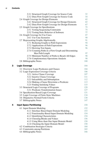
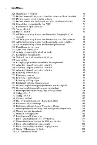
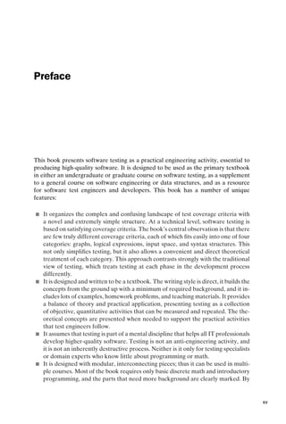
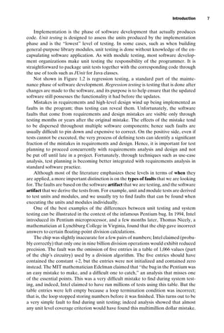
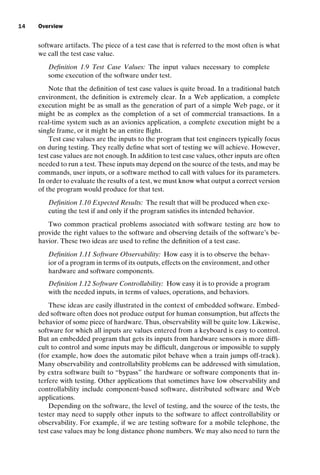
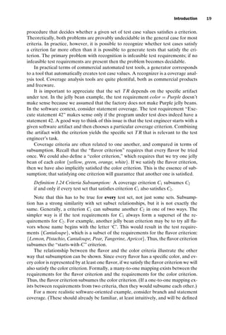
3. Below are four faulty programs. Each includes a test case that results in fail-
ure. Answer the following questions about each program.
public int findLast (int[] x, int y) { public static int lastZero (int[] x) {
//Effects: If x==null throw NullPointerException //Effects: if x==null throw NullPointerException
// else return the index of the last element // else return the index of the LAST 0 in x.
// in x that equals y. // Return -1 if 0 does not occur in x
// If no such element exists, return -1
for (int i=x.length-1; i 0; i--) for (int i = 0; i x.length; i++)
{ {
if (x[i] == y) if (x[i] == 0)
{ {
return i; return i;
} }
} }
return -1; return -1;
} }
// test: x=[2, 3, 5]; y = 2 // test: x=[0, 1, 0]
// Expected = 0 // Expected = 2
public int countPositive (int[] x) { public static int oddOrPos(int[] x) {
//Effects: If x==null throw NullPointerException //Effects: if x==null throw NullPointerException
// else return the number of // else return the number of elements in x that
// positive elements in x. // are either odd or positive (or both)
int count = 0; int count = 0;
for (int i=0; i x.length; i++) for (int i = 0; i x.length; i++)
{ {
if (x[i] = 0) if (x[i]% 2 == 1 || x[i] 0)
{ {
count++; count++;
} }
} }
return count; return count;
} }
// test: x=[-4, 2, 0, 2] // test: x=[-3, -2, 0, 1, 4]
// Expected = 2 // Expected = 3
(a) Identify the fault.
(b) If possible, identify a test case that does not execute the fault.
(c) If possible, identify a test case that executes the fault, but does not result
in an error state.
(d) If possible identify a test case that results in an error, but not a failure.
Hint: Don’t forget about the program counter.
(e) For the given test case, identify the first error state. Be sure to describe
the complete state.
(f) Fix the fault and verify that the given test now produces the expected
output.
1.3 COVERAGE CRITERIA FOR TESTING
Some ill-defined terms occasionally used in testing are “complete testing,” “exhaus-
tive testing,” and “full coverage.” These terms are poorly defined because of a
fundamental theoretical limitation of software. Specifically, the number of poten-
tial inputs for most programs is so large as to be effectively infinite. Consider a
Java compiler – the number of potential inputs to the compiler is not just all Java
programs, or even all almost correct Java programs, but all strings. The only limita-
tion is the size of the file that can be read by the parser. Therefore, the number of
inputs is effectively infinite and cannot be explicitly enumerated.](https://image.slidesharecdn.com/introductiontosoftwaretesting-221201191322-f16668ac/85/Introduction-to-Software-Testing-pdf-40-320.jpg)
![introtest CUUS047-Ammann ISBN 9780521880381 November 8, 2007 17:13 Char Count= 0
22 Overview
first learned that top-down testing is impractical, then OO design pretty much made
the distinction obsolete. The following pair of definitions assumes that software can
be viewed as a tree of software procedures, where the edges represent calls and the
root of the tree is the main procedure.
Definition 1.27 Top-Down Testing: Test the main procedure, then go down
through procedures it calls, and so on.
Definition 1.28 Bottom-Up Testing: Test the leaves in the tree (procedures
that make no calls), and move up to the root. Each procedure is tested only
if all of its children have been tested.
OO software leads to a more general problem. The relationships among classes
can be formulated as general graphs with cycles, requiring test engineers to make
the difficult choice of what order to test the classes in. This problem is discussed in
Chapter 6.
Some parts of the literature separate static and dynamic testing as follows:
Definition 1.29 Static Testing: Testing without executing the program. This
includes software inspections and some forms of analysis.
Definition 1.30 Dynamic Testing: Testing by executing the program with real
inputs.
Most of the literature currently uses “testing” to refer to dynamic testing and
“static testing” is called “verification activities.” We follow that use in this book and
it should be pointed out that this book is only concerned with dynamic or execution-
based testing.
One last term bears mentioning because of the lack of definition. Test Strategy
has been used to mean a variety of things, including coverage criterion, test process,
and technologies used. We will avoid using it.
1.5 BIBLIOGRAPHIC NOTES
All books on software testing and all researchers owe major thanks to the landmark
books in 1979 by Myers [249], in 1990 by Beizer [29], and in 2000 by Binder [33].
Some excellent overviews of unit testing criteria have also been published, including
one by White [349] and more recently by Zhu, Hall, and May [367]. The statement
that software testing requires up to 50 percent of software development costs is from
Myers and Sommerville [249, 316]. The recent text from Pezze and Young [289]
reports relevant processes, principles, and techniques from the testing literature,
and includes many useful classroom materials. The Pezze and Young text presents
coverage criteria in the traditional lifecycle-based manner, and does not organize
criteria into the four abstract models discussed in this chapter.
Numerous other software testing books were not intended as textbooks, or do
not offer general coverage for classroom use. Beizer’s Software System Testing
and Quality Assurance [28] and Hetzel’s The Complete Guide to Software Testing
[160] cover various aspects of management and process for software testing. Several
books cover specific aspects of testing [169, 227, 301]. The STEP project at Georgia](https://image.slidesharecdn.com/introductiontosoftwaretesting-221201191322-f16668ac/85/Introduction-to-Software-Testing-pdf-46-320.jpg)
![introtest CUUS047-Ammann ISBN 9780521880381 November 8, 2007 17:13 Char Count= 0
Introduction 23
Institute of Technology resulted in a comprehensive survey of the practice of soft-
ware testing by Department of Defense contractors in the 1980s [100].
The definition of unit is from Stevens, Myers and Constantine [318], and the def-
inition of module is from Sommerville [316]. The definition of integration testing is
from Beizer [29]. The clarification for OO testing levels with the terms intra-method,
inter-method, and intra-class testing is from Harrold and Rothermel [152] and
inter-class testing is from Gallagher, Offutt and Cincotta [132].
The information for the Pentium bug and Mars lander was taken from several
sources, including by Edelman, Moler, Nuseibeh, Knutson, and Peterson [111, 189,
244, 259, 286]. The accident report [209] is the best source for understanding the
details of the Ariane 5 Flight 501 Failure.
The testing levels in Section 1.1.2 were first defined by Beizer [29].
The elementary result that finding all failures in a program is undecidable is due
to Howden [165].
Most of the terminology in testing is from standards documents, including the
IEEE Standard Glossary of Software Engineering Terminology [175], the US De-
partment of Defense [260, 261], the US Federal Aviation Administration FAA-
DO178B, and the British Computer Society’s Standard for Software Component
Testing [317]. The definitions for observability and controllability come from Freed-
man [129]. Similar definitions were also given in Binder’s book Testing Object-
Oriented Systems [33].
The fault/failure model was developed independently by Offutt and Morell in
their dissertations [101, 246, 247, 262]. Morell used the terms execution, infection,
and propagation [247, 246], and Offutt used reachability, sufficiency, and necessity
[101, 262]. This book merges the two sets of terms by using what we consider to be
the most descriptive terms.
The multiple parts of the test case that we use are based on research in test case
specifications [23, 319].
One of the first discussions of infeasibility from other than a purely theoretical
view was by Frankl and Weyuker [128]. The problem was shown to be undecidable
by Goldberg et al. [136] and DeMillo and Offutt [101]. Some partial solutions have
been presented [132, 136, 177, 273].
Budd and Angluin [51] analyzed the theoretical distinctions between generators
and recognizers from a testing viewpoint. They showed that both problems are for-
mally undecidable, and discussed tradeoffs in approximating the two.
Subsumption has been widely used as a way to analytically compare testing tech-
niques. We follow Weiss [340] and Frankl and Weyuker [128] for our definition
of subsumption. Frankl and Weyuker actually used the term includes. The term
subsumption was defined by Clarke et al.: A criterion C1 subsumes a criterion C2
if and only if every set of execution paths P that satisfies C1 also satisfies C2 [81].
The term subsumption is currently the more widely used and the two definitions are
equivalent; this book follows Weiss’s suggestion to use the term subsumes to refer
to Frankl and Weyuker’s definition.
The descriptions of excise and revenue tasks were taken from Cooper [89].
Although this book does not focus heavily on the theoretical underpinnings of
software testing, students interested in research should study such topics more in
depth. A number of the papers are quite old and often do not appear in current](https://image.slidesharecdn.com/introductiontosoftwaretesting-221201191322-f16668ac/85/Introduction-to-Software-Testing-pdf-47-320.jpg)
![introtest CUUS047-Ammann ISBN 9780521880381 November 8, 2007 17:13 Char Count= 0
24 Overview
literature, and their ideas are beginning to disappear. The authors encourage the
study of the older papers. Among those are truly seminal papers in the 1970s by
Goodenough and Gerhart [138] and Howden [165], and Demillo, Lipton, Sayward,
and Perlis [98, 99]. These papers were followed up and refined by Weyuker and
Ostrand [343], Hamlet [147], Budd and Angluin [51], Gourlay [139], Prather [293],
Howden [168], and Cherniavsky and Smith [67]. Later theoretical papers were con-
tributed by Morell [247], Zhu [366], and Wah [335, 336]. Every PhD student’s ad-
viser will certainly have his or her own favorite theoretical papers, but this list should
provide a good starting point.
NOTES
1 Liskov’s Program Development in Java, especially chapters 9 and 10, is a great source for
students who wish to pursue this direction further.
2 While this is a good general rule, exceptions exist. For example, test requirements for some
logic coverage criteria demand pairs of related test cases instead of individual test cases.
3 The reader might wonder whether we need an Other category to ensure that we have a
partition. In our example, we are ok, but in general, one would need such a category to
handle jelly beans such as Potato, Spinach, or Ear Wax.
4 Correctly answering this question goes a long way towards understanding the weakness of
the subsumption relation.](https://image.slidesharecdn.com/introductiontosoftwaretesting-221201191322-f16668ac/85/Introduction-to-Software-Testing-pdf-48-320.jpg)


![introtest CUUS047-Ammann ISBN 9780521880381 November 8, 2007 17:13 Char Count= 0
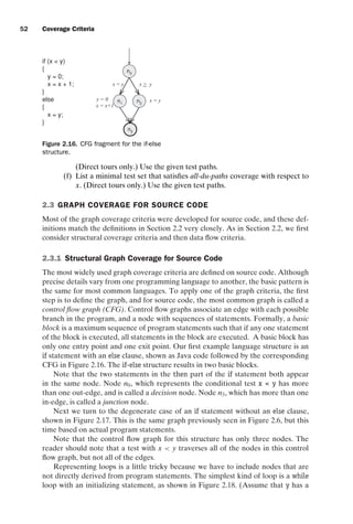
28 Coverage Criteria
N = { n0, n1, n2, n3 }
N0 = { n0 }
E = { (n0, n1), (n0, n2), (n1, n3),(n2, n3 ) }
(a) A graph with a single initial node
N = { n0, n1, n2, n3, n4, n5, n6, n7, n8, n9}
N0 = { n0, n1, n2}
|E| = 12
(b) A graph with mutiple initial nodes
N = { n0, n1, n2, n3 }
|E| = 4
(c) A graph with no initial node
n0
n2
n1
n3
n0
n3
n0 n1 n2
n7 n8 n9
n3 n4 n6
n5 n1 n2
Figure 2.1. Graph (a) has a single initial node, graph (b) multiple initial nodes, and graph (c)
(rejected) with no initial nodes.
N, then for the subgraph defined by Nsub, the set of initial nodes is Nsub ∩ N0, the
set of final nodes is Nsub ∩ Nf , and the set of edges is (Nsub × Nsub) ∩ E.
Note that more than one initial node can be present; that is, N0 is a set. Having
multiple initial nodes is necessary for some software artifacts, for example, if a class
has multiple entry points, but sometimes we will restrict the graph to having one
initial node. Edges are considered to be from one node and to another and written
as (ni , nj ). The edge’s initial node ni is sometimes called the predecessor and nj is
called the successor.
We always identify final nodes, and there must be at least one final node. The
reason is that every test must start in some initial node and end in some final node.
The concept of a final node depends on the kind of software artifact the graph rep-
resents. Some test criteria require tests to end in a particular final node. Other test
criteria are satisfied with any node for a final node, in which case the set Nf is the
same as the set N.
The term node has various synonyms. Graph theory texts sometimes call a node
a vertex, and testing texts typically identify a node with the structure it represents,
often a statement or a basic block. Similarly, graph theory texts sometimes call an
edge an arc, and testing texts typically identify an edge with the structure it repre-
sents, often a branch. This section discusses graph criteria in a generic way; thus we
stick to general graph terms.
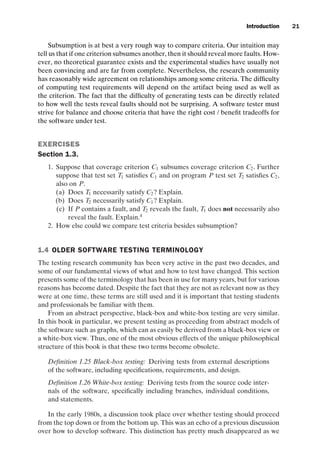
Graphs are often drawn with bubbles and arrows. Figure 2.1 shows three ex-
ample graphs. The nodes with incoming edges but no predecessor nodes are the
initial nodes. The nodes with heavy borders are final nodes. Figure 2.1(a) has a sin-
gle initial node and no cycles. Figure 2.1(b) has three initial nodes, as well as a cycle
([n1, n4, n8, n5, n1]). Figure 2.1(c) has no initial nodes, and so is not useful for gener-
ating test cases.](https://image.slidesharecdn.com/introductiontosoftwaretesting-221201191322-f16668ac/85/Introduction-to-Software-Testing-pdf-52-320.jpg)
![introtest CUUS047-Ammann ISBN 9780521880381 November 8, 2007 17:13 Char Count= 0
Graph Coverage 29
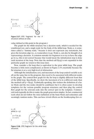
(a) Path examples
(b) Reachability examples
Path Examples
1 n0, n3, n7
2 n1,n4,n8,n5,n1
3 n2, n6, n9
Invalid Path Examples
1 n0, n7
2 n3, n4
3 n2, n6, n8
n0 n2
n7 n9
n3
n1
n8
n4 n6
n5
Reachability Examples
1 reach (n0 ) = N - { n2, n6 }
2 reach (n0, n1, n2) = N
3 reach (n4) = {n1,n4,n5, n7, n8,n9}
4 reach ([n6, n9 ]) = { n9 }
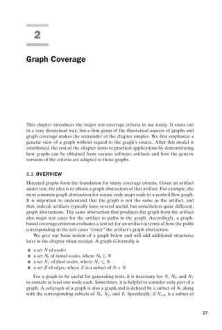
Figure 2.2. Example of paths.
A path is a sequence [n1, n2, . . . , nM] of nodes, where each pair of adjacent nodes,
(ni , ni+1), 1 ≤ i M, is in the set E of edges. The length of a path is defined as the
number of edges it contains. We sometimes consider paths and subpaths of length
zero. A subpath of a path p is a subsequence of p (possibly p itself). Following the
notation for edges, we say a path is from the first node in the path and to the last
node in the path. It is also useful to be able to say that a path is from (or to) an edge
e, which simply means that e is the first (or last) edge in the path.
Figure 2.2 shows a graph along with several example paths, and several examples
that are not paths. For instance, the sequence [n0, n7] is not a path because the two
nodes are not connected by an edge.
Many test criteria require inputs that start at one node and end at another. This
is only possible if those nodes are connected by a path. When we apply these cri-
teria on specific graphs, we sometimes find that we have asked for a path that for
some reason cannot be executed. For example, a path may demand that a loop be
executed zero times in a situation where the program always executes the loop at
least once. This kind of problem is based on the semantics of the software artifact
that the graph represents. For now, we emphasize that we are looking only at the
syntax of the graph.
We say that a node n (or an edge e) is syntactically reachable from node ni if there
exists a path from node ni to n (or edge e). A node n (or edge e) is also semantically
reachable if it is possible to execute at least one of the paths with some input. We can
define the function reachG(x) as the portion of a graph that is syntactically reachable
from the parameter x. The parameter for reachG() can be a node, an edge, or a set of
nodes or edges. Then reachG(ni ) is the subgraph of G that is syntactically reachable
from node ni , reachG(N0) is the subgraph of G that is syntactically reachable from
any initial node, reachG(e) is the subgraph of G syntactically reachable from edge
e, and so on. In our use, reachG() includes the starting nodes. For example, both
reachG(ni ) and reachG([ni , nj ]) always include ni , and reachG([ni , nj ]) includes edge
([ni , nj ]). Some graphs have nodes or starting edges that cannot be syntactically
reached from any of the initial nodes N0. These graphs frustrate attempts to satisfy
a coverage criterion, so we typically restrict our attention to reachG(N0).1](https://image.slidesharecdn.com/introductiontosoftwaretesting-221201191322-f16668ac/85/Introduction-to-Software-Testing-pdf-53-320.jpg)
![introtest CUUS047-Ammann ISBN 9780521880381 November 8, 2007 17:13 Char Count= 0
Graph Coverage 31
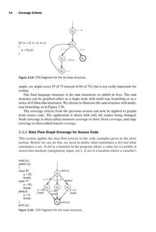
TP1
Test Cases
t1
t3
t2
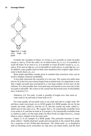
Many-to-one
In deterministic software, a many-to-one relationship
exists between test cases and test paths.
Test Paths
Test Cases
t1
t3
t2
Many-to-many
For nondeterministic software, a many-to-many
relationship exists between test cases and test paths.
TP1
TP3
TP2
t4
Test Paths
TP2
Figure 2.4. Test case mappings to test paths.
node, n6, is designated with a thick circle. Exactly four test paths exist in the
double-diamond graph: [n0, n1, n3, n4, n6], [n0, n1, n3, n5, n6], [n0, n2, n3, n4, n6], and
[n0, n2, n3, n5, n6].
We need some terminology to express the notion of nodes, edges, and subpaths
that appear in test paths, and choose familiar terminology from traveling. A test path
p is said to visit node n if n is in p. Test path p is said to visit edge e if e is in p. The
term visit applies well to single nodes and edges, but sometimes we want to turn our
attention to subpaths. For subpaths, we use the term tour. Test path p is said to tour
subpath q if q is a subpath of p. The first path of Figure 2.3, [n0, n1, n3, n4, n6], visits
nodes n0 and n1, visits edges (n0, n1) and (n3, n4), and tours the subpath [n1, n3, n4]
(among others, these lists are not complete). Since the subpath relationship is re-
flexive, the tour relationship is also reflexive. That is, any given path p always tours
itself.
We define a mapping pathG for tests, so for a test case t, pathG(t) is the test
path in graph G that is executed by t. Since it is usually obvious which graph we are
discussing, we omit the subscript G. We also define the set of paths toured by a set
of tests. For a test set T, path(T) is the set of test paths that are executed by the tests
in T: pathG(T) = { pathG(t)|t ∈ T}.
Except for nondeterministic structures, which we do not consider until Chap-
ter 7, each test case will tour exactly one test path in graph G. Figure 2.4 illustrates
the difference with respect to test case/test path mapping for deterministic vs. non-
deterministic software.
Figure 2.5 illustrates a set of test cases and corresponding test paths on a SESE
graph with the final node nf = n2. Some edges are annotated with predicates that
describe the conditions under which that edge is traversed. (This notion is formal-
ized later in this chapter.) So, in the example, if a is less than b, the only path is from
n0 to n1 and then on to n3 and n2. This book describes all of the graph coverage crite-
ria in terms of relationships of test paths to the graph in question, but it is important
to realize that testing is carried out with test cases, and that the test path is simply a
model of the test case in the abstraction captured by the graph.](https://image.slidesharecdn.com/introductiontosoftwaretesting-221201191322-f16668ac/85/Introduction-to-Software-Testing-pdf-55-320.jpg)
![introtest CUUS047-Ammann ISBN 9780521880381 November 8, 2007 17:13 Char Count= 0
32 Coverage Criteria
(a) Graph for testing the case with input integers
a, b and output (a+b)
(b) Mapping between test cases and test paths
S1
ab
a=b
n0
n1
n3
n2
ab
[ Test path p2 : n0, n3, n2 ]
[ Test path p3
: n0
, n2
]
Test case t1
: (a=0, b=1)
Map to
Test case t2 : (a=1, b=1)
Test case t3
: (a=2, b=1)
[ Test path p1 : n0, n1, n3, n2 ]
Figure 2.5. A set of test cases and corresponding test paths.
EXERCISES
Section 2.1.
1. Give the sets N, N0, Nf , and E for the graph in Figure 2.2.
2. Give a path that is not a test path in Figure 2.2.
3. List all test paths in Figure 2.2.
4. In Figure 2.5, find test case inputs such that the corresponding test path visits
edge (n1, n3).
2.2 GRAPH COVERAGE CRITERIA
The structure in Section 2.1 is adequate to define coverage on graphs. As is usual
in the testing literature, we divide these criteria into two types. The first are usually
referred to as control flow coverage criteria. Because we generalize this situation,
we call them structural graph coverage criteria. The other criteria are based on the
flow of data through the software artifact represented by the graph and are called
data flow coverage criteria. Following the discussion in Chapter 1, we identify the
appropriate test requirements and then define each criterion in terms of the test re-
quirements. In general, for any graph-based coverage criterion, the idea is to identify
the test requirements in terms of various structures in the graph.
For graphs, coverage criteria define test requirements, TR, in terms of properties
of test paths in a graph G. A typical test requirement is met by visiting a particular
node or edge or by touring a particular path. The definitions we have given so far for
a visit are adequate, but the notion of a tour requires more development. We return
to the issue of touring later in this chapter and then refine it further in the context](https://image.slidesharecdn.com/introductiontosoftwaretesting-221201191322-f16668ac/85/Introduction-to-Software-Testing-pdf-56-320.jpg)
![introtest CUUS047-Ammann ISBN 9780521880381 November 8, 2007 17:13 Char Count= 0
Graph Coverage 33
of data flow criteria. The following definition is a refinement of the definition of
coverage given in Chapter 1:
Definition 2.32 Graph Coverage: Given a set TR of test requirements for a
graph criterion C, a test set T satisfies C on graph G if and only if for every
test requirement tr in TR, there is at least one test path p in path(T) such
that p meets tr.
This is a very general statement that must be refined for individual cases.
2.2.1 Structural Coverage Criteria
We specify graph coverage criteria by specifying a set of test requirements, TR. We
will start by defining criteria to visit every node and then every edge in a graph.
The first criterion is probably familiar and is based on the old notion of executing
every statement in a program. This concept has variously been called “statement
coverage,” “block coverage,” “state coverage,” and “node coverage.” We use the
general graph term “node coverage.” Although this concept is familiar and simple,
we introduce some additional notation. The notation initially seems to complicate
the criterion, but ultimately has the effect of making subsequent criteria cleaner and
mathematically precise, avoiding confusion with more complicated situations.
The requirements that are produced by a graph criterion are technically pred-
icates that can have either the value true (the requirement has been met) or false
(the requirement has not been met). For the double-diamond graph in Figure 2.3,
the test requirements for node coverage are: TR = { visit n0, visit n1, visit n2,
visit n3, visit n4, visit n5, visit n6}. That is, we must satisfy a predicate for each node,
where the predicate asks whether the node has been visited or not. With this in
mind, the formal definition of node coverage is as follows2
:
Definition 2.33 Node Coverage (Formal Definition): For each node
n ∈ reachG(N0), TR contains the predicate “visit n.”
This notation, although mathematically precise, is too cumbersome for practical
use. Thus we choose to introduce a simpler version of the definition that abstracts
the issue of predicates in the test requirements.
Criterion 2.1 Node Coverage (NC): TR contains each reachable node in G.
With this definition, it is left as understood that the term “contains” actually
means “contains the predicate visitn.” This simplification allows us to simplify the
writing of the test requirements for Figure 2.3 to only contain the nodes: TR = {n0,
n1, n2, n3, n4, n5, n6}. Test path p1 = [n0, n1, n3, n4, n6] meets the first, second,
fourth, fifth, and seventh test requirements, and test path p2 = [n0, n2, n3, n5, n6]
meets the first, third, fourth, sixth, and seventh. Therefore, if a test set T contains
{t1, t2}, where path(t1) = p1 and path(t2) = p2, then T satisfies node coverage on G.
The usual definition of node coverage omits the intermediate step of explicitly
identifying the test requirements, and is often stated as given below. Notice the
economy of the form used above with respect to the standard definition. Several](https://image.slidesharecdn.com/introductiontosoftwaretesting-221201191322-f16668ac/85/Introduction-to-Software-Testing-pdf-57-320.jpg)
![introtest CUUS047-Ammann ISBN 9780521880381 November 8, 2007 17:13 Char Count= 0
34 Coverage Criteria
path (t1
) = [ n0
, n1
, n2
]
path (t2
) = [ n0
, n2
]
n0
n1
n2
x y
x y
T1 = { t1 }
T1 satisfies node coverage on the graph
(a) Node Coverage
T2 = { t1 , t2 }
T2 satisfies edge coverage on the graph
(b) Edge Coverage
Figure 2.6. A graph showing node coverage and edge coverage.
of the exercises emphasize this point by directing the student to recast other criteria
in the standard form.
Definition 2.34 Node Coverage (NC) (Standard Definition): Test set T satis-
fies node coverage on graph G if and only if for every syntactically reachable
node n in N, there is some path p in path(T) such that p visits n.
The exercises at the end of the section have the reader reformulate the defini-
tions of some of the remaining coverage criteria in both the formal way and the
standard way. We choose the intermediate definition because it is more compact,
avoids the extra verbiage in a standard coverage definition, and focuses just on the
part of the definition of coverage that changes from criterion to criterion.
Node coverage is implemented in many commercial testing tools, most often in
the form of statement coverage. So is the next common criterion of edge coverage,
usually implemented as branch coverage:
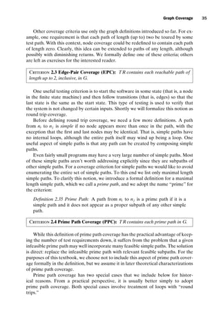
Criterion 2.2 Edge Coverage (EC): TR contains each reachable path of length
up to 1, inclusive, in G.
The reader might wonder why the test requirements for edge coverage also ex-
plicitly include the test requirements for node coverage – that is, why the phrase
“up to” is included in the definition. In fact, all the graph coverage criteria are de-
veloped like this. The motivation is subsumption for graphs that do not contain more
complex structures. For example, consider a graph with a node that has no edges.
Without the “up to” clause in the definition, edge coverage would not cover that
node. Intuitively, we would like edge testing to be at least as demanding as node
testing. This style of definition is the best way to achieve this property. To make our
TR sets readable, we list only the maximal length paths.
Figure 2.6 illustrates the difference between node and edge coverage. In program
statement terms, this is a graph of the common “if-else” structure.](https://image.slidesharecdn.com/introductiontosoftwaretesting-221201191322-f16668ac/85/Introduction-to-Software-Testing-pdf-58-320.jpg)
![introtest CUUS047-Ammann ISBN 9780521880381 November 8, 2007 17:13 Char Count= 0
36 Coverage Criteria
A round trip path is a prime path of nonzero length that starts and ends at the
same node. One type of round trip test coverage requires at least one round trip
path to be taken for each node, and another requires all possible round trip paths.
Criterion 2.5 Simple Round Trip Coverage (SRTC): TR contains at least one
round-trip path for each reachable node in G that begins and ends a round-trip
path.
Criterion 2.6 Complete Round Trip Coverage (CRTC): TR contains all round-
trip paths for each reachable node in G.
Next we turn to path coverage, which is traditional in the testing literature.
Criterion 2.7 Complete Path Coverage (CPC): TR contains all paths in G.
Sadly, complete path coverage is useless if a graph has a cycle, since this results
in an infinite number of paths, and hence an infinite number of test requirements.
A variant of this criterion is, however, useful. Suppose that instead of requiring all
paths, we consider a specified set of paths. For example, these paths might be given
by a customer in the form of usage scenarios.
Criterion 2.8 Specified Path Coverage (SPC): TR contains a set S of test paths,
where S is supplied as a parameter.
Complete path coverage is not feasible for graphs with cycles; hence the reason
for developing the other alternatives listed above. Figure 2.7 contrasts prime path
coverage with complete path coverage. Part (a) of the figure shows the “diamond”
graph, which contains no loops. Both complete path coverage and prime path cov-
erage can be satisfied on this graph with the two paths shown. Part (b), however,
includes a loop from n1 to n3 to n4 to n1, thus the graph has an infinite number of
possible test paths, and complete path coverage is not possible. The requirements
for prime path coverage, however, can be toured with two test paths, for example,
[n0, n1, n2] and [n0, n1, n3, n4, n1, n3, n4, n1, n2].
Touring, Sidetrips, and Detours
An important but subtle point to note is that while simple paths do not have internal
loops, we do not require the test paths that tour a simple path to have this property.
That is, we distinguish between the path that specifies a test requirement and the
portion of the test path that meets the requirement. The advantage of separating
these two notions has to do with the issue of infeasible test requirements. Before
describing this advantage, let us refine the notion of a tour.
We previously defined “visits” and “tours,” and recall that using a path p to tour
a subpath [n1, n2, n3] means that the subpath is a subpath of p. This is a rather strict
definition because each node and edge in the subpath must be visited exactly in the
order that they appear in the subpath. We would like to relax this a bit to allow](https://image.slidesharecdn.com/introductiontosoftwaretesting-221201191322-f16668ac/85/Introduction-to-Software-Testing-pdf-60-320.jpg)
![introtest CUUS047-Ammann ISBN 9780521880381 November 8, 2007 17:13 Char Count= 0
Graph Coverage 37
(a) Prime Path Coverage on a
Graph with No Loops
(b) Prime Path Coverage on a
Graph with Loops
Prime Paths = { [n0, n1, n3], [n0, n2, n3] }
path (t1) = [n0, n1, n3]
path (t2) = [n0, n2, n3]
T1 = {t1, t2}
T1 satisfies prime path coverage on the graph
Prime Paths = { [n0, n1, n2],
[n0, n1, n3, n4], [n1, n3, n4, n1],
[n3, n4, n1, n3], [n4, n1, n3, n4],
[n3, n4, n1, n2] }
path (t3) = [n0, n1, n2]
path (t4) = [n0, n1, n3, n4, n1, n3, n4, n1, n2]
T2 = {t3, t4}
T2 satisfies prime path coverage on the graph
n0
n2
n1
n3
n0
n3
n1
n2
n4
Figure 2.7. Two graphs showing prime path coverage.
loops to be included in the tour. Consider the graph in Figure 2.8, which features a
small loop from b to c and back.
If we are required to tour subpath q = [a, b, d], the strict definition of tour
prohibits us from meeting the requirement with any path that contains c, such as
p = [s0, a, b, c, b, d, s f ], because we do not visit a, b, and d in exactly the same or-
der. We relax the tour definition in two ways. The first allows the tour to include
“sidetrips,” where we can leave the path temporarily from a node and then return
to the same node. The second allows the tour to include more general “detours”
where we can leave the path from a node and then return to the next node on the
S0 a b
c
Sf
d
Figure 2.8. Graph with a loop.](https://image.slidesharecdn.com/introductiontosoftwaretesting-221201191322-f16668ac/85/Introduction-to-Software-Testing-pdf-61-320.jpg)
![introtest CUUS047-Ammann ISBN 9780521880381 November 8, 2007 17:13 Char Count= 0
38 Coverage Criteria
S0
a b
c
Sf
d
S0
a b
c
Sf
d
(a) Graph being toured with a sidetrip
(b) Graph being toured with a detour
1
4
3
6
5
2
1
3
4
5
2
Figure 2.9. Tours, sidetrips, and detours in graph coverage.
path (skipping an edge). In the following definitions, q is a required subpath that is
assumed to be simple.
Definition 2.36 Tour: Test path p is said to tour subpath q if and only if q is
a subpath of p.
Definition 2.37 Tour with Sidetrips: Test path p is said to tour subpath q with
sidetrips if and only if every edge in q is also in p in the same order.
Definition 2.38 Tour with Detours: Test path p is said to tour subpath q with
detours if and only if every node in q is also in p in the same order.
The graphs in Figure 2.9 illustrate sidetrips and detours on the graph from Fig-
ure 2.8. In Figure 2.9(a), the dashed lines show the sequence of edges that are exe-
cuted in a tour with a sidetrip. The numbers on the dashed lines indicate the order in
which the edges are executed. In Figure 2.9(b), the dashed lines show the sequence
of edges that are executed in a tour with a detour.
While these differences are rather small, they have far-reaching consequences.
The difference between sidetrips and detours can be seen in Figure 2.9. The subpath
[b, c, b] is a sidetrip to [a, b, d] because it leaves the subpath at node b and then
returns to the subpath at node b. Thus, every edge in the subpath [a, b, d] is executed
in the same order. The subpath [b, c, d] is a detour to [a, b, d] because it leaves
the subpath at node b and then returns to a node in the subpath at a later point,
bypassing the edge (b, d). That is, every node [a, b, d] is executed in the same order
but every edge is not. Detours have the potential to drastically change the behavior
of the intended test. That is, a test that takes the edge (c, d) may exhibit different](https://image.slidesharecdn.com/introductiontosoftwaretesting-221201191322-f16668ac/85/Introduction-to-Software-Testing-pdf-62-320.jpg)
![introtest CUUS047-Ammann ISBN 9780521880381 November 8, 2007 17:13 Char Count= 0
Graph Coverage 39
behavior and test different aspects of the program than a test that takes the edge
(b, d).
To use the notion of sidetrips and detours, one can “decorate” each appropriate
graph coverage criterion with a choice of touring. For example, prime path coverage
could be defined strictly in terms of tours, less strictly to allow sidetrips, or even less
strictly to allow detours.
The position taken in this book is that sidetrips are a practical way to deal with
infeasible test requirements, as described below. Hence we include them explicitly
in our criteria. Detours seem less practical, and so we do not include them further.
Dealing with Infeasible Test Requirements
If sidetrips are not allowed, a large number of infeasible requirements can exist.
Consider again the graph in Figure 2.9. In many programs it will be impossible to
take the path from a to d without going through node c at least once because, for
example, the loop body is written such that it cannot be skipped. If this happens,
we need to allow sidetrips. That is, it may not be possible to tour the path [a, b, d]
without a sidetrip.
The argument above suggests dropping the strict notion of touring and simply
allowing test requirements to be met with sidetrips. However, this is not always a
good idea! Specifically, if a test requirement can be met without a sidetrip, then
doing so is clearly superior to meeting the requirement with a sidetrip. Consider the
loop example again. If the loop can be executed zero times, then the path [a, b, d]
should be toured without a sidetrip.
The argument above suggests a hybrid treatment with desirable practical and
theoretical properties. The idea is to meet test requirements first with strict tours,
and then allow sidetrips for unmet test requirements. Clearly, the argument could
easily be extended to detours, but, as mentioned above, we elect not to do so.
Definition 2.39 Best Effort Touring: Let TRtour be the subset of test require-
ments that can be toured and TRsidetrip be the subset of test requirements
that can be toured with sidetrips. Note that TRtour ⊆ TRsidetrip. A set T of test
paths achieves best effort touring if for every path p in TRtour, some path in
T tours p directly and for every path p in TRsidetrip, some path in T tours p
either directly or with a sidetrip.
Best-effort touring has the practical benefit that as many test requirements are
met as possible, yet each test requirement is met in the strictest possible way. As we
will see in Section 2.2.3 on subsumption, best-effort touring has desirable theoretical
properties with respect to subsumption.
Finding Prime Test Paths
It turns out to be relatively simple to find all prime paths in a graph, and test paths
to tour the prime paths can be constructed in a mechanical manner. Consider the
example graph in Figure 2.10. It has seven nodes and nine edges, including a loop
and an edge from node n4 to itself (sometimes called a “self-loop.”)
Prime paths can be found by starting with paths of length 0, then extending to
length 1, and so on. Such an algorithm collects all simple paths, whether prime or](https://image.slidesharecdn.com/introductiontosoftwaretesting-221201191322-f16668ac/85/Introduction-to-Software-Testing-pdf-63-320.jpg)
![introtest CUUS047-Ammann ISBN 9780521880381 November 8, 2007 17:13 Char Count= 0
40 Coverage Criteria
n0
n4
n1
n6
n5
n2
n3
Figure 2.10. An example for prime
test paths.
not. The prime paths can be easily screened from this set. The set of paths of length
0 is simply the set of nodes, and the set of paths of length 1 is simply the set of edges.
For simplicity, we simply list the node numbers in this example.
Simple paths of length 0 (7):
1) [0]
2) [1]
3) [2]
4) [3]
5) [4]
6) [5]
7) [6] !
The exclamation point on the path [6] tells us that this path cannot be extended.
Specifically, the final node 6 has no outgoing edges, and so paths that end with 6 are
not extended further.
Simple paths of length 1 (9):
8) [0, 1]
9) [0, 4]
10) [1, 2]
11) [1, 5]
12) [2, 3]
13) [3, 1]
14) [4, 4] *
15) [4, 6] !
16) [5, 6] !
The asterisk on the path [4, 4] tells us that path can go no further because the
first node is the same as the last (it is already a cycle). For paths of length 2, we
identify each path of length 1 that is not a cycle (marked with asterisks). We then
extend the path with every node that can be reached from the final node in the path
unless that node is already in the path and not the first node. The first path of length
1, [0, 1], is extended to [0, 1, 2] and [0, 1, 5]. The second, [0, 4], is extended to [0, 4, 6]
but not [0, 4, 4], because node 4 is already in the path ([0, 4, 4] is not simple and thus
is not prime).](https://image.slidesharecdn.com/introductiontosoftwaretesting-221201191322-f16668ac/85/Introduction-to-Software-Testing-pdf-64-320.jpg)
![introtest CUUS047-Ammann ISBN 9780521880381 November 8, 2007 17:13 Char Count= 0
Graph Coverage 41
Simple paths of length 2 (8):
17) [0, 1, 2]
18) [0, 1, 5]
19) [0, 4, 6] !
20) [1, 2, 3]
21) [1, 5, 6] !
22) [2, 3, 1]
23) [3, 1, 2]
24) [3, 1, 5]
Paths of length 3 are computed in a similar way.
Simple paths of length 3 (7):
25) [0, 1, 2, 3] !
26) [0, 1, 5, 6] !
27) [1, 2, 3, 1] *
28) [2, 3, 1, 2] *
29) [2, 3, 1, 5]
30) [3, 1, 2, 3] *
31) [3, 1, 5, 6] !
Finally, only one path of length 4 exists. Three paths of length 3 cannot be ex-
tended because they are cycles; two others end with node 6. Of the remaining two,
the path that ends in node 3 cannot be extended because [0, 1, 2, 3, 1] is not simple
and thus is not prime.
Prime paths of length 4 (1):
32) [2, 3, 1, 5, 6]!
The prime paths can be computed by eliminating any path that is a (proper) sub-
path of some other simple path. Note that every simple path without an exclamation
mark or asterisk is eliminated as it can be extended and is thus a proper subpath of
some other simple path. There are eight prime paths:
14) [4, 4] *
19) [0, 4, 6] !
25) [0, 1, 2, 3] !
26) [0, 1, 5, 6] !
27) [1, 2, 3, 1] *
28) [2, 3, 1, 2] *
30) [3, 1, 2, 3] *
32) [2, 3, 1, 5, 6]!
This process is guaranteed to terminate because the length of the longest pos-
sible prime path is the number of nodes. Although graphs often have many simple
paths (32 in this example, of which 8 are prime), they can usually be toured with
far fewer test paths. Many possible algorithms can find test paths to tour the prime
paths. Observation will suffice with a graph as simple as in Figure 2.10. For example,
it can be seen that the four test paths [0, 1, 5, 6], [0, 1, 2, 3, 1, 2, 3, 1, 5, 6], [0, 4, 6],](https://image.slidesharecdn.com/introductiontosoftwaretesting-221201191322-f16668ac/85/Introduction-to-Software-Testing-pdf-65-320.jpg)
![introtest CUUS047-Ammann ISBN 9780521880381 November 8, 2007 17:13 Char Count= 0
42 Coverage Criteria
and [0, 4, 4, 6] are enough. This approach, however, is error-prone. The easiest thing
to do is to tour the loop [1, 2, 3] only once, which omits the prime paths [2, 3, 1, 2]
and [3, 1, 2, 3].
With more complicated graphs, a mechanical approach is needed. We recom-
mend starting with the longest prime paths and extending them to the begin-
ning and end nodes in the graph. For our example, this results in the test path
[0, 1, 2, 3, 1, 5, 6]. The test path [0, 1, 2, 3, 1, 5, 6] tours 3 prime paths 25, 27, and 32.
The next test path is constructed by extending one of the longest remaining
prime paths; we will continue to work backward and choose 30. The resulting test
path is [0, 1, 2, 3, 1, 2, 3, 1, 5, 6], which tours 2 prime paths, 28 and 30 (it also tours
paths 25 and 27).
The next test path is constructed by using the prime path 26 [0, 1, 5, 6]. This test
path tours only maximal prime path 26.
Continuing in this fashion yields two more test paths, [0, 4, 6] for prime path 19,
and [0, 4, 4, 6] for prime path 14.
The complete set of test paths is then:
1) [0, 1, 2, 3, 1, 5, 6]
2) [0, 1, 2, 3, 1, 2, 3, 1, 5, 6]
3) [0, 1, 5, 6]
4) [0, 4, 6]
5) [0, 4, 4, 6]
This can be used as is, or optimized if the tester desires a smaller test set. It
is clear that test path 2 tours the prime paths toured by test path 1, so 1 can be
eliminated, leaving the four test paths identified informally earlier in this section.
Simple algorithms can automate this process.
EXERCISES
Section 2.2.1.
1. Redefine edge coverage in the standard way (see the discussion for node cov-
erage).
2. Redefine complete path coverage in the standard way (see the discussion for
node coverage).
3. Subsumption has a significant weakness. Suppose criterion Cstrong subsumes
criterion Cweak and that test set Tstrong satisfies Cstrong and test set Tweak satisfies
Cweak. It is not necessarily the case that Tweak is a subset of Tstrong. It is also not
necessarily the case that Tstrong reveals a fault if Tweak reveals a fault. Explain
these facts.
4. Answer questions (a)–(d) for the graph defined by the following sets:
N = {1, 2, 3, 4}
N0 = {1}
Nf = {4}
E = {(1, 2), (2, 3), (3, 2), (2, 4)}](https://image.slidesharecdn.com/introductiontosoftwaretesting-221201191322-f16668ac/85/Introduction-to-Software-Testing-pdf-66-320.jpg)
![introtest CUUS047-Ammann ISBN 9780521880381 November 8, 2007 17:13 Char Count= 0
Graph Coverage 43
(a) Draw the graph.
(b) List test paths that achieve node coverage, but not edge coverage.
(c) List test paths that achieve edge coverage, but not edge Pair coverage.
(d) List test paths that achieve edge pair coverage.
5. Answer questions (a)–(g) for the graph defined by the following sets:
N = {1, 2, 3, 4, 5, 6, 7}
N0 = {1}
Nf = {7}
E = {(1, 2), (1, 7), (2, 3), (2, 4), (3, 2), (4, 5), (4, 6), (5, 6), (6, 1)}
Also consider the following (candidate) test paths:
t0 = [1, 2, 4, 5, 6, 1, 7]
t1 = [1, 2, 3, 2, 4, 6, 1, 7]
(a) Draw the graph.
(b) List the test requirements for edge-pair coverage. (Hint: You should get
12 requirements of length 2).
(c) Does the given set of test paths satisfy edge-pair coverage? If not, identify
what is missing.
(d) Consider the simple path [3, 2, 4, 5, 6] and test path [1, 2, 3, 2, 4, 6, 1,
2, 4, 5, 6, 1, 7]. Does the test path tour the simple path directly? With a
sidetrip? If so, identify the sidetrip.
(e) List the test requirements for node coverage, edge coverage, and prime
path coverage on the graph.
(f) List test paths that achieve node coverage but not edge coverage on the
graph.
(g) List test paths that achieve edge coverage but not prime path coverage on
the graph.
6. Answer questions (a)–(c) for the graph in Figure 2.2.
(a) Enumerate the test requirements for node coverage, edge coverage, and
prime path coverage on the graph.
(b) List test paths that achieve node coverage but not edge coverage on the
graph.
(c) List test paths that achieve edge coverage but not prime path coverage
on the graph.
7. Answer questions (a)–(d) for the graph defined by the following sets:
N = {0, 1, 2}
N0 = {0}
Nf = {2}
E = {(0, 1), (0, 2), (1, 0), (1, 2), (2, 0)}
Also consider the following (candidate) paths:
p0 = [0, 1, 2, 0]
p1 = [0, 2, 0, 1, 2]
p2 = [0, 1, 2, 0, 1, 0, 2]
p3 = [1, 2, 0, 2]
p4 = [0, 1, 2, 1, 2]
(a) Which of the listed paths are test paths? Explain the problem with any
path that is not a test path.](https://image.slidesharecdn.com/introductiontosoftwaretesting-221201191322-f16668ac/85/Introduction-to-Software-Testing-pdf-67-320.jpg)
![introtest CUUS047-Ammann ISBN 9780521880381 November 8, 2007 17:13 Char Count= 0
44 Coverage Criteria
ab
a=b
n0
n1
n3
n2
ab
use (n2
) = { a, b }
def (n3
) = { b }
def (n0
) = { a,b }
use (n0
, n1
) = { a, b }
use (n0
, n2
) = { a, b }
use (n0 , n3 ) = { a, b }
Figure 2.11. A graph showing variables, def sets and use sets.
(b) List the eight test requirements for edge-pair coverage (only the length
two subpaths).
(c) Does the set of test paths (part a) above satisfy edge-pair coverage? If
not, identify what is missing.
(d) Consider the prime path [n2, n0, n2] and path p2. Does p2 tour the prime
path directly? With a sidetrip?
8. Design and implement a program that will compute all prime paths in a graph,
then derive test paths to tour the prime paths. Although the user interface can
be arbitrarily complicated, the simplest version will be to accept a graph as
input by reading a list of nodes, initial nodes, final nodes, and edges.
2.2.2 Data Flow Criteria
The next few testing criteria are based on the assumption that to test a program
adequately, we should focus on the flows of data values. Specifically, we should
try to ensure that the values created at one point in the program are created and
used correctly. This is done by focusing on definitions and uses of values. A defini-
tion (def) is a location where a value for a variable is stored into memory (assign-
ment, input, etc.). A use is a location where a variable’s value is accessed. Data flow
testing criteria use the fact that values are carried from defs to uses. We call these
du-pairs (they are also known as definition-use, def-use, and du associations in the
testing literature). The idea of data flow criteria is to exercise du-pairs in various
ways.
First we must integrate data flow into the existing graph model. Let V be a set of
variables that are associated with the program artifact being modeled in the graph.
Each node n and edge e is considered to define a subset of V; this set is called def(n)
or def(e). (Although graphs from programs cannot have defs on edges, other soft-
ware artifacts such as finite state machines can allow defs as side effects on edges.)
Each node n and edge e is also considered to use a subset of V; this set is called
use(n) or use(e).
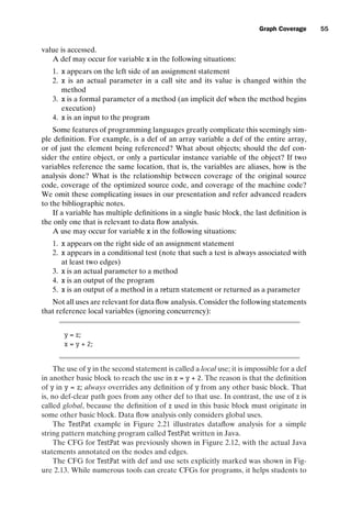
Figure 2.11 gives an example of a graph annotated with defs and uses. All vari-
ables involved in a decision are assumed to be used on the associated edges, so a
and b are in the use set of all three edges (n0, n1), (n0, n2), and (n0, n3).](https://image.slidesharecdn.com/introductiontosoftwaretesting-221201191322-f16668ac/85/Introduction-to-Software-Testing-pdf-68-320.jpg)
![introtest CUUS047-Ammann ISBN 9780521880381 November 8, 2007 17:13 Char Count= 0
Graph Coverage 45
An important concept when discussing data flow criteria is that a def of a variable
may or may not reach a particular use. The most obvious reason that a def of a
variable v at location li (a location could be a node or an edge) will not reach a use
at location lj is because no path goes from li to lj . A more subtle reason is that the
variable’s value may be changed by another def before it reaches the use. Thus, a
path from li to lj is def-clear with respect to variable v if for every node nk and every
edge ek on the path, k = i and k = j, v is not in def(nk) or in def(ek). That is, no
location between li and lj changes the value. If a def-clear path goes from li to lj
with respect to v, we say that the def of v at li reaches the use at lj .
For simplicity, we will refer to the start and end of a du-path as nodes, even if the
definition or the use occurs on an edge. We discuss relaxing this convention later.
Formally, a du-path with respect to a variable v is a simple path that is def-clear
with respect to v from a node ni for which v is in def(ni ) to a node nj for which v is
in use(nj ). We want the paths to be simple to ensure a reasonably small number of
paths. Note that a du-path is always associated with a specific variable v, a du-path
always has to be simple, and there may be intervening uses on the path.
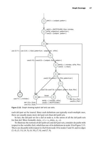
Figure 2.12 gives an example of a graph annotated with defs and uses. Rather
than displaying the actual sets, we show the full program statements that are asso-
ciated with the nodes and edges. This is common and often more informative to a
human, but the actual sets are simpler for automated tools to process. Note that the
parameters (subject and pattern) are considered to be explicitly defined by the first
node in the graph. That is, the def set of node 1 is def(1) = {subject, pattern}. Also
note that decisions in the program (for example, if subject[iSub] == pattern[0]) re-
sult in uses of each of the associated variables for both edges in the decision. That
is, use(4, 10) ≡ use(4,5) ≡ {subject, iSub, pattern}. The parameter subject is used at
node 2 (with a reference to its length attribute) and at edges (4, 5), (4, 10), (7, 8), and
(7, 9), thus du-paths exist from node 1 to node 2 and from node 1 to each of those
four edges.
Figure 2.13 shows the same graph, but this time with the def and use sets explic-
itly marked on the graph.3
Note that node 9 both defines and uses the variable iPat.
This is because of the statement iPat ++, which is equivalent to iPat = iPat+1. In
this case, the use occurs before the def, so for example, a def-clear path goes from
node 5 to node 9 with respect to iPat.
The test criteria for data flow will be defined as sets of du-paths. This makes the
criteria quite simple, but first we need to categorize the du-paths into several groups.
The first grouping of du-paths is according to definitions. Specifically, consider
all of the du-paths with respect to a given variable defined in a given node. Let the
def-path set du(ni , v) be the set of du-paths with respect to variable v that start at
node ni . Once we have clarified the notion of touring for dataflow coverage, we will
define the All-Defs criterion by simply asking that at least one du-path from each
def-path set be toured. Because of the large number of nodes in a typical graph,
and the potentially large number of variables defined at each node, the number of
def-path sets can be quite large. Even so, the coverage criterion that arises from the
def-path groupings tends to be quite weak.
Perhaps surprisingly, it is not helpful to group du-paths by uses, and so we will
not provide a definition of “use-path” sets that parallels the definition of def-path
sets given above.](https://image.slidesharecdn.com/introductiontosoftwaretesting-221201191322-f16668ac/85/Introduction-to-Software-Testing-pdf-69-320.jpg)
![introtest CUUS047-Ammann ISBN 9780521880381 November 8, 2007 17:13 Char Count= 0
46 Coverage Criteria
1
2
4
3
5
6
7
8 9
10
11
NOTFOUND = -1
iSub = 0
rtnIndex = NOTFOUND
isPat = false
subjectLen = subject.length
patternLen = pattern.length
iSub + patternLen - 1 subjectLen
isPat = = false
(iSub + patternLen - 1 = subjectLen ||
isPat != false )
subject [iSub] == pattern [0]
iSub++
(subject [iSub] != pattern [0])
rtnIndex = iSub
isPat = true
iPat = 1
iPat patternLen
iPat = patternLen
subject[iSub + iPat] !=
pattern[iPat]
subject[iSub + iPat] ==
pattern[iPat]
iPat++
break
rtnIndex = NOTFOUND
isPat = false;
return (rtnIndex)
subject, pattern are forwarded
parameters
Figure 2.12. A graph showing an example of du-paths.
The second, and more important, grouping of du-paths is according to pairs of
definitions and uses. We call this the def-pair set. After all, the heart of data flow
testing is allowing definitions to flow to uses. Specifically, consider all of the du-paths
with respect to a given variable that are defined in one node and used in another
(possibly identical) node. Formally, let the def-pair set du(ni , nj , v) be the set of du-
paths with respect to variable v that start at node ni and end at node nj . Informally,
a def-pair set collects together all the (simple) ways to get from a given definition
to a given use. Once we have clarified the notion of touring for dataflow coverage,
we will define the All-Uses criterion by simply asking that at least one du-path from](https://image.slidesharecdn.com/introductiontosoftwaretesting-221201191322-f16668ac/85/Introduction-to-Software-Testing-pdf-70-320.jpg)
![introtest CUUS047-Ammann ISBN 9780521880381 November 8, 2007 17:13 Char Count= 0
48 Coverage Criteria
The def-path set for the use of isub at node 10 is:
du(10, iSub) = {[10, 3, 4], [10, 3, 4, 5], [10, 3, 4, 5, 6, 7, 8], [10, 3, 4, 5, 6, 7, 9],
[10, 3, 4, 5, 6, 10], [10, 3, 4, 5, 6, 7, 8, 10], [10, 3, 4, 10],
[10, 3, 11]}
This def-path set can be broken up into the following def-pair sets:
du(10, 4, iSub) = is{[10, 3, 4]}
du(10, 5, iSub) = {[10, 3, 4, 5]}
du(10, 8, iSub) = {[10, 3, 4, 5, 6, 7, 8]}
du(10, 9, iSub) = {[10, 3, 4, 5, 6, 7, 9]}
du(10, 10, iSub) = {[10, 3, 4, 5, 6, 10], [10, 3, 4, 5, 6, 7, 8, 10], [10, 3, 4, 10]}
du(10, 11, iSub) = {[10, 3, 11]}
Next, we extend the definition of tour to apply to du-paths. A test path p is
said to du tour subpath d with respect to v if p tours d and the portion of p to
which d corresponds is def-clear with respect to v. Depending on how one wishes to
define the coverage criteria, one can either allow or disallow def-clear sidetrips with
respect to v when touring a du-path. Because def-clear sidetrips make it possible to
tour more du-paths, we define the dataflow coverage criteria given below to allow
sidetrips where necessary.
Now we can define the primary data flow coverage criteria. The three most com-
mon are best understood informally. The first requires that each def reaches at least
one use, the second requires that each def reaches all possible uses, and the third
requires that each def reaches all possible uses through all possible du-paths. As
mentioned in the development of def-path sets and def-pair sets, the formal def-
initions of the criteria are simply appropriate selections from the appropriate set.
For each test criterion below, we assume best effort touring (see Section 2.2.1),
where sidetrips are required to be def-clear with respect to the variable in ques-
tion.
Criterion 2.9 All-Defs Coverage (ADC): For each def-path set S = du(n, v), TR
contains at least one path d in S.
Remember that the def-path set du(n, v) represents all def-clear simple paths
from n to all uses of v. So All-Defs requires us to tour at least one path to at least
one use.
Criterion 2.10 All-Uses Coverage (AUC): For each def-pair set S = du(ni , nj ,
v), TR contains at least one path d in S.
Remember that the def-pair set du(ni , nj , v) represents all the def-clear simple
paths from a def of v at ni to a use of v at nj . So All-Uses requires us to tour at least
one path for every def-use pair.4
Criterion 2.11 All-du-Paths Coverage (ADUPC): For each def-pair set S = du
(ni , nj , v), TR contains every path d in S.
The definition could also simply be written as “include every du-path.” We chose
the given formulation because it highlights that the key difference between All-Uses](https://image.slidesharecdn.com/introductiontosoftwaretesting-221201191322-f16668ac/85/Introduction-to-Software-Testing-pdf-72-320.jpg)
![introtest CUUS047-Ammann ISBN 9780521880381 November 8, 2007 17:13 Char Count= 0
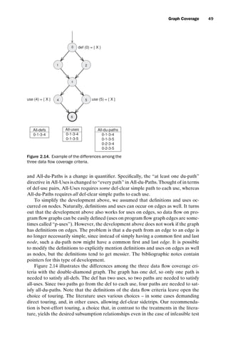
Graph Coverage 51
coverage, then we will have implicitly ensured that every def was used. Thus All-
Defs is also satisfied and All-Uses subsumes All-Defs. Likewise, if we satisfy All-du-
Paths coverage, then we will have implicitly ensured that every def reached every
possible use. Thus All-Uses is also satisfied and All-du-Paths subsumes All-Uses.
Additionally, each edge is based on the satisfaction of some predicate, so each edge
has at least one use. Therefore All-Uses will guarantee that each edge is executed
at least once, so All-Uses subsumes edge coverage.
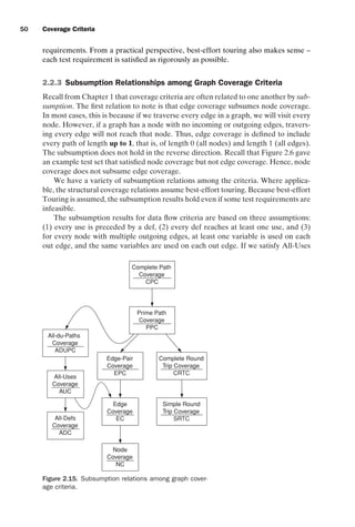
Finally, each du-path is also a simple path, so prime path coverage subsumes All-
du-Paths coverage.5
This is a significant observation, since computing prime paths is
considerably simpler than analyzing data flow relationships. Figure 2.15 shows the
subsumption relationships among the structural and data flow coverage criteria.
EXERCISES
Section 2.2.3.
1. Below are four graphs, each of which is defined by the sets of nodes, initial
nodes, final nodes, edges, and defs and uses. Each graph also contains a col-
lection of test paths. Answer the following questions about each graph.
Graph I. Graph II.
N = {0, 1, 2, 3, 4, 5, 6, 7} N = {1, 2, 3, 4, 5, 6}
N0 = {0} N0 = {1}
Nf = {7} Nf = {6}
E = {(0, 1), (1, 2), (1, 7), (2, 3), (2, 4), (3, 2), E = {(1, 2), (2, 3), (2, 6), (3, 4), (3, 5), (4, 5), (5, 2)}
(4, 5), (4, 6), (5, 6), (6, 1)} def (x) = {1, 3}
def (0) = def (3) = use(5) = use(7) = {x} use(x) = {3, 6} // Assume the use of x in 3 precedes
the def
Test Paths: Test Paths:
t1 = [0, 1, 7] t1 = [1, 2, 6]
t2 = [0, 1, 2, 4, 6, 1, 7] t2 = [1, 2, 3, 4, 5, 2, 3, 5, 2, 6]
t3 = [0, 1, 2, 4, 5, 6, 1, 7] t3 = [1, 2, 3, 5, 2, 3, 4, 5, 2, 6]
t4 = [0, 1, 2, 3, 2, 4, 6, 1, 7] t4 = [1, 2, 3, 5, 2, 6]
t5 = [0, 1, 2, 3, 2, 3, 2, 4, 5, 6, 1, 7]
t6 = [0, 1, 2, 3, 2, 4, 6, 1, 2, 4, 5, 6, 1, 7]
Graph III. Graph IV.
N = {1, 2, 3, 4, 5, 6} N = {1, 2, 3, 4, 5, 6}
N0 = {1} N0 = {1}
Nf = {6} Nf = {6}
E = {(1, 2), (2, 3), (3, 4), (3, 5), (4, 5), (5, 2), (2, 6)} E = {(1, 2), (2, 3), (2, 6), (3, 4), (3, 5), (4, 5),
def (x) = {1, 4} (5, 2)}
use(x) = {3, 5, 6} def (x) = {1, 5}
use(x) = {5, 6} // Assume the use of x in 5 pre-
cedes the def
Test Paths: Test Paths:
t1 = [1, 2, 3, 5, 2, 6] t1 = [1, 2, 6]
t2 = [1, 2, 3, 4, 5, 2, 6] t2 = [1, 2, 3, 4, 5, 2, 3, 5, 2, 6]
t3 = [1, 2, 3, 5, 2, 3, 4, 5, 2, 6]
(a) Draw the graph.
(b) List all of the du-paths with respect to x. (Note: Include all du-paths, even
those that are subpaths of some other du-path).
(c) For each test path, determine which du-paths that test path tours. For this
part of the exercise, you should consider both direct touring and sidetrips.
Hint: A table is a convenient format for describing this relationship.
(d) List a minimal test set that satisfies all-defs coverage with respect to x.
(Direct tours only.) Use the given test paths.
(e) List a minimal test set that satisfies all-uses coverage with respect to x.](https://image.slidesharecdn.com/introductiontosoftwaretesting-221201191322-f16668ac/85/Introduction-to-Software-Testing-pdf-75-320.jpg)
![introtest CUUS047-Ammann ISBN 9780521880381 November 8, 2007 17:13 Char Count= 0
56 Coverage Criteria
// Example program for pattern matching of two strings
class TestPat
{
public static void main (String[] argv)
{
final int MAX = 100;
char subject[] = new char[MAX];
char pattern[] = new char[MAX];
if (argv.length != 2)
{
System.out.println
(java TestPat String-Subject String-Pattern);
return;
}
subject = argv[0].toCharArray();
pattern = argv[1].toCharArray();
TestPat testPat = new TestPat ();
int n = 0;
if ((n = testPat.pat (subject, pattern)) == -1)
System.out.println
(Pattern string is not a substring of the subject string);
else
System.out.println
(Pattern string begins at the character + n);
}
public TestPat ()
{ }
public int pat (char[] subject, char[] pattern)
{
// Post: if pattern is not a substring of subject, return -1
// else return (zero-based) index where the pattern (first)
// starts in subject
final int NOTFOUND = -1;
int iSub = 0, rtnIndex = NOTFOUND;
boolean isPat = false;
int subjectLen = subject.length;
int patternLen = pattern.length;
while (isPat == false iSub + patternLen - 1 subjectLen)
{
if (subject [iSub] == pattern [0])
{
rtnIndex = iSub; // Starting at zero
isPat = true;
for (int iPat = 1; iPat patternLen; iPat ++)
{
if (subject[iSub + iPat] != pattern[iPat])
{
rtnIndex = NOTFOUND;
isPat = false;
break; // out of for loop
}
}
}
iSub ++;
}
return (rtnIndex);
}
}
Figure 2.21. TestPat for data flow example.
create CFGs by hand. When doing so, a good habit is to draw the CFG first with the
statements, then redraw it with the def and use sets.
Table 2.1 lists the defs and uses at each node in the CFG for TestPat This sim-
ply repeats the information in Figure 2.13, but in a convenient form. Table 2.2 con-
tains the same information for edges. We suggest that beginning students check their](https://image.slidesharecdn.com/introductiontosoftwaretesting-221201191322-f16668ac/85/Introduction-to-Software-Testing-pdf-80-320.jpg)
, [2,3,4,5,6,10](iSub), and [2,3,4,5,6,7,8,10](iSub).
Table 2.2. Defs and uses at each edge in the CFG for TestPat.
edge use
(1, 2)
(2, 3)
(3, 4) {iSub, patternLen, subjectLen, isPat}
(3, 11) {iSub, patternLen, subjectLen, isPat}
(4, 5) {subject, iSub, pattern}
(4, 10) {subject, iSub, pattern}
(5, 6)
(6, 7) {iPat, patternLen}
(6, 10) {iPat, patternLen}
(7, 8) {subject, iSub, iPat, pattern}
(7, 9) {subject, iSub, iPat, pattern}
(8, 10)
(9, 6)
(10, 3)](https://image.slidesharecdn.com/introductiontosoftwaretesting-221201191322-f16668ac/85/Introduction-to-Software-Testing-pdf-81-320.jpg)
![introtest CUUS047-Ammann ISBN 9780521880381 November 8, 2007 17:13 Char Count= 0
58 Coverage Criteria
Table 2.3. Du-path sets for each variable in TestPat
variable du-path set du-paths prefix?
NOTFOUND du (2, NOTFOUND) [2,3,4,5,6,7,8]
rtnIndex du (2, rtnIndex) [2,3,11]
du (5, rtnIndex) [5,6,10,3,11]
du (8, rtnIndex) [8,10,3,11]
iSub du (2, iSub) [2,3,4] Yes
[2,3,4,5] Yes
[2,3,4,5,6,7,8] Yes
[2,3,4,5,6,7,9]
[2,3,4,5,6,10]
[2,3,4,5,6,7,8,10]
[2,3,4,10]
[2,3,11]
du (10, iSub) [10,3,4] Yes
[10,3,4,5] Yes
[10,3,4,5,6,7,8] Yes
[10,3,4,5,6,7,9]
[10,3,4,5,6,10]
[10,3,4,5,6,7,8,10]
[10,3,4,10]
[10,3,11]
iPat du (5, iPat) [5,6,7] Yes
[5,6,10]
[5,6,7,8]
[5,6,7,9]
du (9, iPat) [9,6,7] Yes
[9,6,10]
[9,6,7,8]
[9,6,7,9]
isPat du (2, isPat) [2,3,4]
[2,3,11]
du (5, isPat) [5,6,10,3,4]
[5,6,10,3,11]
du (8, isPat) [8,10,3,4]
[8,10,3,11]
subject du (1, subject) [1,2] Yes
[1,2,3,4,5] Yes
[1,2,3,4,10]
[1,2,3,4,5,6,7,8]
[1,2,3,4,5,6,7,9]
pattern du (1, pattern) [1,2] Yes
[1,2,3,4,5] Yes
[1,2,3,4,10]
[1,2,3,4,5,6,7,8]
[1,2,3,4,5,6,7,9]
subjectLen du (2, subjectLen) [2,3,4]
[2,3,11]
patternLen du (2, patternLen) [2,3,4] Yes
[2,3,11]
[2,3,4,5,6,7]
[2,3,4,5,6,10]](https://image.slidesharecdn.com/introductiontosoftwaretesting-221201191322-f16668ac/85/Introduction-to-Software-Testing-pdf-82-320.jpg)
![introtest CUUS047-Ammann ISBN 9780521880381 November 8, 2007 17:13 Char Count= 0
Graph Coverage 59
Table 2.4. Test paths to satisfy all du-paths coverage on TestPat
test case test path(t)
(subject,pattern,output)
(a, bc, −1) [1,2,3,11]
(ab, a, 0) [1,2,3,4,5,6,10,3,11]
(ab, ab, 0 ) [1,2,3,4,5,6,7,9,6,10,3,11]
(ab, ac, −1) [1,2,3,4,5,6,7,8,10,3,11]
(ab, b, 1) [1,2,3,4,10,3,4,5,6,10,3,11]
(ab, c, −1) [1,2,3,4,10,3,4,10,3,11]
(abc, abc, 0) [1,2,3,4,5,6,7,9,6,7,9,6,10,3,11]
(abc, abd, −1) [1,2,3,4,5,6,7,9,6,7,8,10,3,11]
(abc, ac −1) [1,2,3,4,5,6,7,8,10,3,4,10,3,11]
(abc, ba, −1) [1,2,3,4,10,3,4,5,6,7,8,10,3,11]
(abc, bc, 1) [1,2,3,4,10,3,4,5,6,7,9,6,10,3,11]
One optimization uses the fact that a du-path must be toured by any test that
tours an extension of that du-path. These du-paths are marked with the annotation
“Yes” in the prefix? column of the table. For example, [2,3,4](iSub) is necessarily
toured by any test that tours the du-path [2,3,4,5,6,7,8](iSub), because [2,3,4] is a
prefix of [2,3,4,5,6,7,8]. Thus, the path is not considered in the subsequent table that
relates du-paths to test paths that tour them. One has to be a bit careful with this
optimization, since the extended du-path may be infeasible even if the prefix is not.
Table 2.4 shows that a relatively small set of 11 test cases satisfies all du-paths
coverage on this example. (One du-path is infeasible.) The reader may wish to eval-
uate this test set with the non-data flow graph coverage criteria.
Table 2.5 lists which du-paths are toured by each test case. For each test case in
the first column, the test path that is executed by that test is shown in the second
column, and the du-path that is toured by the test path is shown in the third column.
Table 2.5. Test paths and du-paths covered on TestPat.
test case test path(t) du-path toured
(subject,pattern,
output)
(ab, ac, −1) [1,2,3,4,5,6,7,8,10,3,11] [2,3,4,5,6,7,8](NOTFOUND)
(a, bc, −1) [1,2,3,11] [2,3,11](rtnIndex)
(ab, a, 0) [1,2,3,4,5,6,10,3,11] [5,6,10,3,11](rtnIndex)
(ab, ac, −1) [1,2,3,4,5,6,7,8,10,3,11] [8,10,3,11](rtnIndex)
(ab, ab, 0 ) [1,2,3,4,5,6,7,9,6,10,3,11] [2,3,4,5,6,7,9] (iSub)
(ab, a, 0) [1,2,3,4,5,6,10,3,11] [2,3,4,5,6,10](iSub)
(ab, ac, −1) [1,2,3,4,5,6,7,8,10,3,11] [2,3,4,5,6,7,8,10](iSub)
(ab, c, −1) [1,2,3,4,10,3,4,10,3,11] [2,3,4,10](iSub)
(a, bc, −1) [1,2,3,11] [2,3,11] (iSub)
(abc, bc, 1) [1,2,3,4,10,3,4,5,6,7,9,6,10,3,11] [10,3,4,5,6,7,9](iSub)
(ab, b, 1) [1,2,3,4,10,3,4,5,6,10,3,11] [10,3,4,5,6,10](iSub)
(abc, ba, −1) [1,2,3,4,10,3,4,5,6,7,8,10,3,11] [10,3,4,5,6,7,8,10](iSub)
(ab, c, −1) [1,2,3,4,10,3,4,10,3,11] [10,3,4,10](iSub)](https://image.slidesharecdn.com/introductiontosoftwaretesting-221201191322-f16668ac/85/Introduction-to-Software-Testing-pdf-83-320.jpg)
![introtest CUUS047-Ammann ISBN 9780521880381 November 8, 2007 17:13 Char Count= 0
60 Coverage Criteria
Table 2.5. Continued
test case test path(t) du-path toured
(subject,pattern,
output)
(ab, a, 0) [1,2,3,4,5,6,10,3,11] [10,3,11](iSub)
(ab, a, 0) [1,2,3,4,5,6,10,3,11] [5,6,10](iPat)
(ab, ac, −1) [1,2,3,4,5,6,7,8,10,3,11] [5,6,7,8](iPat)
(ab, ab, 0 ) [1,2,3,4,5,6,7,9,6,10,3,11] [5,6,7,9](iPat)
(ab, ab, 0 ) [1,2,3,4,5,6,7,9,6,10,3,11] [9,6,10](iPat)
(abc, abd, −1) [1,2,3,4,5,6,7,9,6,7,8,10,3,11] [9,6,7,8](iPat)
(abc, abc, 0) [1,2,3,4,5,6,7,9,6,7,9,6,10,3,11] [9,6,7,9](iPat)
(ab, ac, −1) [1,2,3,4,5,6,7,8,10,3,11] [2,3,4](isPat)
(a, bc, −1) [1,2,3,11] [2,3,11](isPat)
No test case Infeasible [5,6,10,3,4](isPat)
(ab, a, 0) [1,2,3,4,5,6,10,3,11] [5,6,10,3,11](isPat)
(abc, ac −1) [1,2,3,4,5,6,7,8,10,3,4,10,3,11] [8,10,3,4](isPat)
(ab, ac, −1) [1,2,3,4,5,6,7,8,10,3,11] [8,10,3,11](isPat)
(ab, c, −1) [1,2,3,4,10,3,4,10,3,11] [1,2,3,4,10](subject)
(ab, ac, −1) [1,2,3,4,5,6,7,8,10,3,11] [1,2,3,4,5,6,7,8](subject)
(ab, ab, 0 ) [1,2,3,4,5,6,7,9,6,10,3,11] [1,2,3,4,5,6,7,9](subject)
(ab, c, −1) [1,2,3,4,10,3,4,10,3,11] [1,2,3,4,10](pattern)
(ab, ac, −1) [1,2,3,4,5,6,7,8,10,3,11] [1,2,3,4,5,6,7,8](pattern)
(ab, ab, 0 ) [1,2,3,4,5,6,7,9,6,10,3,11] [1,2,3,4,5,6,7,9](pattern)
(ab, c, −1) [1,2,3,4,10,3,4,10,3,11] [2,3,4](subjectLen)
(a, bc, −1) [1,2,3,11] [2,3,11](subjectLen)
(a, bc, −1) [1,2,3,11] [2,3,11](patternLen)
(ab, ac, −1) [1,2,3,4,5,6,7,8,10,3,11] [2,3,4,5,6,7](patternLen)
(ab, a, 0) [1,2,3,4,5,6,10,3,11] [2,3,4,5,6,10](patternLen)
EXERCISES
Section 2.3.
1. Use the following program fragment for questions (a)–(e) below.
w = x; // node 1
if (m 0)
{
w++; // node 2
}
else
{
w=2*w; // node 3
}
// node 4 (no executable statement)
if (y = 10)
{
x = 5*y; // node 5
}
else](https://image.slidesharecdn.com/introductiontosoftwaretesting-221201191322-f16668ac/85/Introduction-to-Software-Testing-pdf-84-320.jpg)
![introtest CUUS047-Ammann ISBN 9780521880381 November 8, 2007 17:13 Char Count= 0
Graph Coverage 61
{
x = 3*y+5; // node 6
}
z = w + x; // node 7
(a) Draw a control flow graph for this program fragment. Use the node num-
bers given above.
(b) Which nodes have defs for variable w?
(c) Which nodes have uses for variable w?
(d) Are there any du-paths with respect to variable w from node 1 to node 7?
If not, explain why not. If any exist, show one.
(e) Enumerate all of the du-paths for variables w and x.
2. Select a commercial coverage tool of your choice. Note that some have free
trial evaluations. Choose a tool, download it, and run it on some software.
You can use one of the examples from this text, software from your work
environment, or software available over the Web. Write up a short sum-
mary report of your experience with the tool. Be sure to include any prob-
lems installing or using the tool. The main grading criterion is that you
actually collect some coverage data for a reasonable set of tests on some
program.
3. Consider the pattern matching example in Figure 2.21. Instrument the code
so as to be able to produce the execution paths reported in the text for this
example. That is, on a given test execution, your instrumentation program
should compute and print the corresponding test path. Run the instrumented
program on the test cases listed at the end of Section 2.3.
4. Consider the pattern matching example in Figure 2.21. In particular, consider
the final table of tests in Section 2.3. Consider the variable iSub. Number the
(unique) test cases, starting at 1, from the top of the iSub part of the table.
For example, (ab, c, −1), which appears twice in the iSub portion of the table,
should be labeled test t4.
(a) Give a minimal test set that satisfies all defs coverage. Use the test cases
given.
(b) Give a minimal test set that satisfies all uses coverage.
(c) Give a minimal test set that satisfies all du-paths coverage.
5. Again consider the pattern matching example in Figure 2.21. Instrument the
code so as to produce the execution paths reported in the text for this exam-
ple. That is, on a given test execution, your tool should compute and print
the corresponding test path. Run the following three test cases and answer
questions (a)–(g) below:
subject = “brown owl” pattern = “wl” expected output = 7
subject = “brown fox” pattern = “dog” expected output = −1
subject = “fox” pattern = “brown” expected output = −1
(a) Find the actual path followed by each test case.
(b) For each path, give the du-paths that the path tours in the table at the
end of Section 2.3. To reduce the scope of this exercise, consider only the
following du-paths: du (10, iSub), du (2, isPat), du (5, isPat), and du (8,
isPat).
(c) Explain why the du-path [5, 6, 10, 3, 4] cannot be toured by any test path.](https://image.slidesharecdn.com/introductiontosoftwaretesting-221201191322-f16668ac/85/Introduction-to-Software-Testing-pdf-85-320.jpg)
![introtest CUUS047-Ammann ISBN 9780521880381 November 8, 2007 17:13 Char Count= 0
62 Coverage Criteria
(d) Select tests from the table at the end of Section 2.3 to complete coverage
of the (feasible) du-paths that are uncovered in question a.
(e) From the tests above, find a minimal set of tests that achieves All-Defs
coverage with respect to the variable isPat.
(f) From the tests above, find a minimal set of tests that achieves All-Uses
Coverage with respect to the variable isPat.
(g) Is there any difference between All-Uses coverage and all du-paths cov-
erage with respect to the variable isPat in the pat method?
6. Use the following method fmtRewrap() for questions a–e below.
1. /** *****************************************************
2. * Rewraps the string (Similar to the Unix fmt).
3. * Given a string S, eliminate existing CRs and add CRs to the
4. * closest spaces before column N. Two CRs in a row are considered to
5. * be hard CRs and are left alone.
7. ********************************************************/
6.
8. static final char CR = ’n’;
9. static final int inWord = 0;
10. static final int betweenWord = 1;
11. static final int lineBreak = 2;
12. static final int crFound = 3;
13. static private String fmtRewrap (String S, int N)
14. {
15. int state = betweenWord;
16. int lastSpace = -1;
17. int col = 1;
18. int i = 0;
19. char c;
20.
21. char SArr [] = S.toCharArray();
22. while (i S.length())
23. {
24. c = SArr[i];
25. col++;
26. if (col = N)
27. state = lineBreak;
28. else if (c == CR)
29. state = crFound;
30. else if (c == ’ ’)
31. state = betweenWord;
32. else
33. state = inWord;
34. switch (state)
35. {
36. case betweenWord:](https://image.slidesharecdn.com/introductiontosoftwaretesting-221201191322-f16668ac/85/Introduction-to-Software-Testing-pdf-86-320.jpg)
![introtest CUUS047-Ammann ISBN 9780521880381 November 8, 2007 17:13 Char Count= 0
Graph Coverage 63
37. lastSpace = i;
38. break;
39.
40. case lineBreak:
41. SArr [lastSpace] = CR;
42. col = i-lastSpace;
43. break;
44.
45. case crFound:
46. if (i+1 S.length() SArr[i+1] == CR)
47. {
48. i++; // Two CRs = hard return
49. col = 1;
50. }
51. else
52. SArr[i] = ’’;
53. break;
54.
55. case inWord:
56. default:
57. break;
58. } // end switch
59. i++;
60. } // end while
61. S = new String (SArr) + CR;
62. return (S);
63. }
(a) Draw the control flow graph for the fmtRewrap() method.
(b) For fmtRewrap(), find a test case such that the corresponding test path
visits the edge that connects the beginning of the while statement to the
S = new String(SArr) + CR; statement without going through the body
of the while loop.
(c) Enumerate the test requirements for node coverage, edge coverage, and
prime path coverage for the graph for fmtRewrap().
(d) List test paths that achieve node coverage but not edge coverage on the
graph.
(e) List test paths that achieve edge coverage but not prime path coverage on
the graph.
7. Use the following method printPrimes() for questions a–f below.
1. /** *****************************************************
2. * Finds and prints n prime integers
3. * Jeff Offutt, Spring 2003
4. ********************************************************* */
5. private static void printPrimes (int n)
6. {](https://image.slidesharecdn.com/introductiontosoftwaretesting-221201191322-f16668ac/85/Introduction-to-Software-Testing-pdf-87-320.jpg)
![introtest CUUS047-Ammann ISBN 9780521880381 November 8, 2007 17:13 Char Count= 0
64 Coverage Criteria
7. int curPrime; // Value currently considered for primeness
8. int numPrimes; // Number of primes found so far.
9. boolean isPrime; // Is curPrime prime?
10. int [] primes = new int [MAXPRIMES]; // The list of prime numbers.
11.
12. // Initialize 2 into the list of primes.
13. primes [0] = 2;
14. numPrimes = 1;
15. curPrime = 2;
16. while (numPrimes n)
17. {
18. curPrime++; // next number to consider ...
19. isPrime = true;
20. for (int i = 0; i = numPrimes-1; i++)
21. { // for each previous prime.
22. if (isDivisible (primes[i], curPrime))
23. { // Found a divisor, curPrime is not prime.
24. isPrime = false;
25. break; // out of loop through primes.
26. }
27. }
28. if (isPrime)
29. { // save it!
30. primes[numPrimes] = curPrime;
31. numPrimes++;
32. }
33. } // End while
34.
35. // Print all the primes out.
36. for (int i = 0; i = numPrimes-1; i++)
37. {
38. System.out.println (Prime: + primes[i]);
39. }
40. } // end printPrimes
(a) Draw the control flow graph for the printPrimes() method.
(b) Consider test cases t1 = (n = 3) and t2 = (n = 5). Although these tour the
same prime paths in printPrimes(), they do not necessarily find the same
faults. Design a simple fault that t2 would be more likely to discover than
t1 would.
(c) For printPrimes(), find a test case such that the corresponding test
path visits the edge that connects the beginning of the while state-
ment to the for statement without going through the body of the while
loop.
(d) Enumerate the test requirements for node coverage, edge coverage, and
prime path coverage for the graph for printPrimes().](https://image.slidesharecdn.com/introductiontosoftwaretesting-221201191322-f16668ac/85/Introduction-to-Software-Testing-pdf-88-320.jpg)
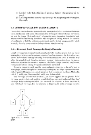
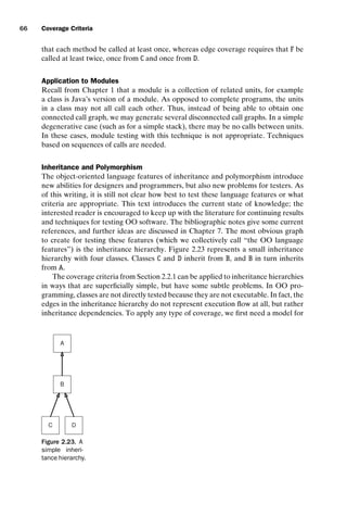
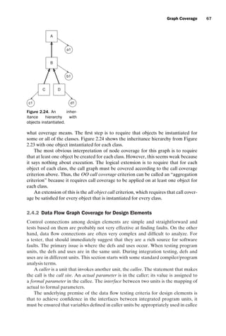
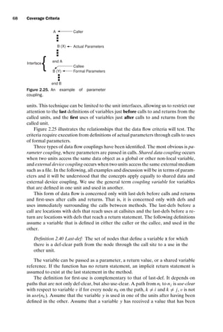
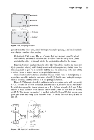
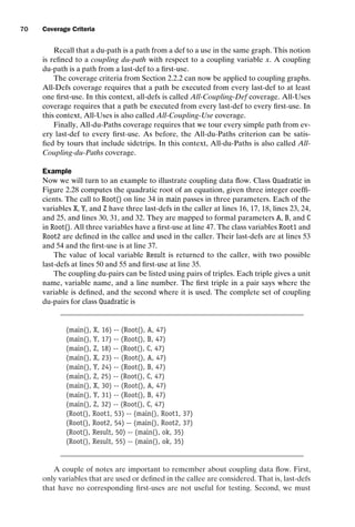
![introtest CUUS047-Ammann ISBN 9780521880381 November 8, 2007 17:13 Char Count= 0
Graph Coverage 71
1 // Program to compute the quadratic root for two numbers
2 import java.lang.Math;
3
4 class Quadratic
5 {
6 private static double Root1, Root2;
7
8 public static void main (String[] argv)
9 {
10 int X, Y, Z;
11 boolean ok;
12 if (argv.length == 3)
13 {
14 try
15 {
16 X = Integer.parseInt (argv[1]);
17 Y = Integer.parseInt (argv[2]);
18 Z = Integer.parseInt (argv[3]);
19 }
20 catch (NumberFormatException e)
21 {
22 System.out.println (Inputs not integers, using 8, 10, -33.);
23 X = 8;
24 Y = 10;
25 Z = -33;
26 }
27 }
28 else
29 {
30 X = 8;
31 Y = 10;
32 Z = -33;
33 }
34 ok = Root (X, Y, Z);
35 if (ok)
36 System.out.println
37 (Quadratic: Root 1 = + Root1 + , Root 2 = + Root2);
38 else
39 System.out.println (No solution.);
40 }
41
42 // Finds the quadratic root, A must be non-zero
43 private static boolean Root (int A, int B, int C)
44 {
45 double D;
46 boolean Result;
47 D = (double)(B*B) - (double)(4.0*A*C);
48 if (D 0.0)
49 {
50 Result = false;
51 return (Result);
52 }
53 Root1 = (double) ((-B + Math.sqrt(D)) / (2.0*A));
54 Root2 = (double) ((-B - Math.sqrt(D)) / (2.0*A));
55 Result = true;
56 return (Result);
57 } // End method Root
58
59 } // End class Quadratic
Figure 2.28. Quadratic root program.
remember implicit initialization of class and global variables. In some languages
(such as Java and C), class and instance variables are given default values. These def-
initions can be modeled as occurring at the beginning of appropriate units. For ex-
ample, class-level initializations may be considered to occur in the main() method or
in constructors. Although other methods that access class variables may use the de-
fault values on the first call, it is also possible for such methods to use values written
by other methods, and hence the normal coupling data flow analysis methods should](https://image.slidesharecdn.com/introductiontosoftwaretesting-221201191322-f16668ac/85/Introduction-to-Software-Testing-pdf-95-320.jpg)
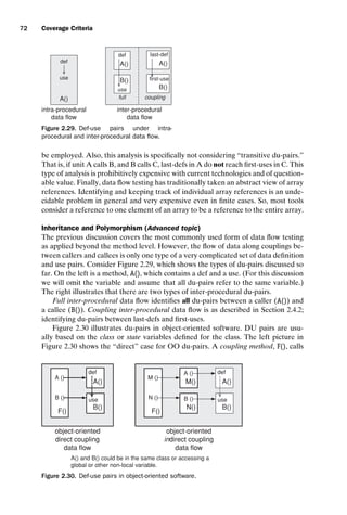
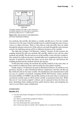

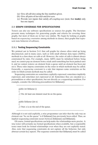
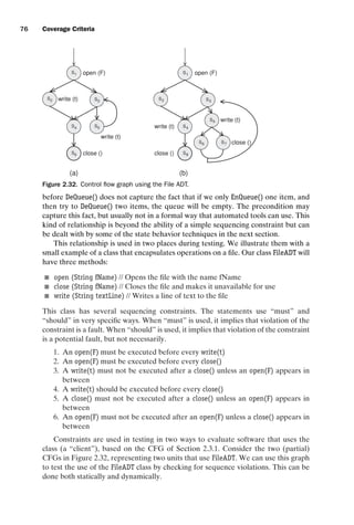
![introtest CUUS047-Ammann ISBN 9780521880381 November 8, 2007 17:13 Char Count= 0
Graph Coverage 77
Static checks (not considered to be traditional testing) proceed by checking each
constraint. First consider the write(t) statements at nodes 2 and 5 in graph (a). We
can check to see whether paths exist from the open(F) at node 1 to nodes 2 and 5
(constraint 1). We can also check whether a path exists from the open(F) at node 1
to the close() at node 6 (constraint 2). For constraints 3 and 4, we can check to see
if a path goes from the close() at node 6 to any of the write(t) statements, and see
if a path exists from the open(F) to the close() that does not go through at least one
write(t). This will uncover one possible problem, the path [1, 3, 4, 6] goes from an
open(F) to a close() with no intervening write(t) calls.
For constraint 5, we can check if a path exists from a close() to a close() that does
not go through an open(F). For constraint 6, we can check if a path exists from an
open(F) to an open(F) that does not go through a close().
This process will find a more serious problem with graph (b) in 2.32. A path exists
from the close() at node 7 to the write(t) at node 5 and to the write(t) at node 4. While
this may seem simple enough not to require formalism for such small graphs, this
process is quite difficult with large graphs containing dozens or hundreds of nodes.
Dynamic testing follows a slightly different approach. Consider the problem in
graph (a) where no write() appears on the possible path [1, 3, 4, 6]. It is quite pos-
sible that the logic of the program dictates that the edge (3, 4) can never be taken
unless the loop [3, 5, 3] is taken at least once. Because deciding whether the path
[1, 3, 4, 6] can be taken or not is formally undecidable, this situation can be checked
only by dynamic execution. Thus we generate test requirements to try to violate the
sequencing constraints. For the FileADT class, we generate the following sets of test
requirements:
1. Cover every path from the start node to every node that contains a write(t)
such that the path does not go through a node containing an open(F).
2. Cover every path from the start node to every node that contains a close()
such that the path does not go through a node containing an open(F).
3. Cover every path from every node that contains a close() to every node that
contains a write(t) such that the path does not contain an open(F).
4. Cover every path from every node that contains an open(F) to every node that
contains a close() such that the path does not go through a node containing a
write(t).
5. Cover every path from every node that contains an open(F) to every node that
contains an open(F).
Of course, all of these test requirements will be infeasible in well written programs.
However, any tests created as a result of these requirements will almost certainly
reveal a fault if one exists.
2.5.2 Testing State Behavior of Software
The other major method for using graphs based on specifications is to model state
behavior of the software by developing some form of finite state machine (FSM).
Over the last 25 years, many suggestions have been made for creating FSMs and how
to test software based on the FSM. The topic of how to create, draw, and interpret a](https://image.slidesharecdn.com/introductiontosoftwaretesting-221201191322-f16668ac/85/Introduction-to-Software-Testing-pdf-101-320.jpg)
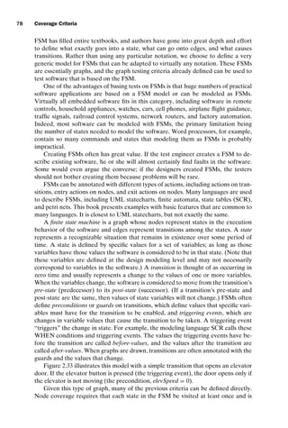
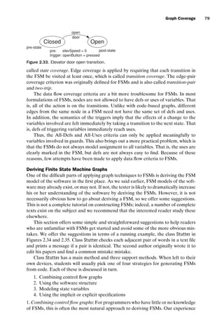
![introtest CUUS047-Ammann ISBN 9780521880381 November 8, 2007 17:13 Char Count= 0
80 Coverage Criteria
/** *****************************************************
// Stutter checks for repeat words in a text file.
// It prints a list of repeat words, by line number.
// Stutter will accept standard input or a list
// of file names.
// Jeff Offutt, June 1989 (in C), Java version March 2003
//********************************************************* */
class Stutter
{
// Class variables used in multiple methods.
private static boolean lastdelimit = true;
private static String curWord = , prevWord = ;
private static char delimits [] =
{’’, ’ ’, ’,’, ’.’, ’!’, ’-’, ’+’, ’=’, ’;’, ’:’, ’?’,
’’, ’{’, ’}’, ’’}; // First char in list is a tab
//************************************************
// main parses the arguments, decides if stdin
// or a file name, and calls Stut().
//************************************************
public static void main (String[] args) throws IOException
{
String fileName;
FileReader myFile;
BufferedReader inFile = null;
if (args.length == 0)
{ // no file, use stdin
inFile = new BufferedReader (new InputStreamReader (System.in));
}
else
{
fileName = args [0];
if (fileName == null)
{ // no file name, use stdin
inFile = new BufferedReader (new InputStreamReader (System.in));
}
else
{ // file name, open the file.
myFile = new FileReader (fileName);
inFile = new BufferedReader (myFile);
}
}
stut (inFile);
}
//************************************************
// Stut() reads all lines in the input stream, and
// finds words. Words are defined as being surrounded
// by delimiters as defined in the delimits[] array.
// Every time an end of word is found, checkDupes()
// is called to see if it is the same as the
// previous word.
//************************************************
private static void stut (BufferedReader inFile) throws IOException
{
String inLine;
char c;
int linecnt = 1;
Figure 2.34. Stutter – Part A.
has been that the majority of students will use this approach if not guided away from
it. A control flow graph-based FSM for class Stutter is given in Figure 2.36.
The graph in Figure 2.36 is not a FSM at all, and this is not the way to
form graphs from software. This method has several problems, the first being that
the nodes are not states. The methods must return to the appropriate callsites,
which means that the graphs contain built-in nondeterminism. For example, in](https://image.slidesharecdn.com/introductiontosoftwaretesting-221201191322-f16668ac/85/Introduction-to-Software-Testing-pdf-104-320.jpg)
![introtest CUUS047-Ammann ISBN 9780521880381 November 8, 2007 17:13 Char Count= 0
Graph Coverage 81
while ((inLine = inFile.readLine()) != null)
{ // For each line
for (int i=0; iinLine.length(); i++)
{ // for each character
c = inLine.charAt(i);
if (isDelimit (c))
{ // Found an end of a word.
checkDupes (linecnt);
}
else
{
lastdelimit = false;
curWord = curWord + c;
}
}
linecnt++;
checkDupes (linecnt);
}
} // end Stut
//************************************************
// checkDupes() checks to see if the globally defined
// curWord is the same as prevWord and prints a message
// if they are the same.
//************************************************
private static void checkDupes (int line)
{
if (lastdelimit)
return; // already checked, keep skipping
lastdelimit = true;
if (curWord.equals(prevWord))
{
System.out.println (Repeated word on line + line + : +
prevWord+ + curWord);
}
else
{
prevWord = curWord;
}
curWord = ;
} // end checkDupes
//************************************************
// Checks to see if a character is a delimiter.
//************************************************
private static boolean isDelimit (char C)
{
for (int i = 0; i delimits.length; i++)
if (C == delimits [i])
return (true);
return (false);
}
} // end class Stutter
Figure 2.35. Stutter – Part B.
Figure 2.36, there is an edge from node 2 in checkDupes() to node 6 in stut(), and
also an edge from node 2 in checkDupes() to node 8 in stut(). Which edge is taken
depends on whether the edge from node 6 in stut() was taken to enter checkDupes()
or the edge from node 8 in stut() was taken to enter checkDupes(). Second, the
implementation must be finished before the graph can be built; remember from
Chapter 1 that one of our goals is to prepare tests as early as possible. Most im-
portantly, however, this kind of graph does not scale to large software products. The
graph is complicated enough with small Stutter and gets much worse with larger pro-
grams.](https://image.slidesharecdn.com/introductiontosoftwaretesting-221201191322-f16668ac/85/Introduction-to-Software-Testing-pdf-105-320.jpg)
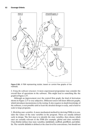
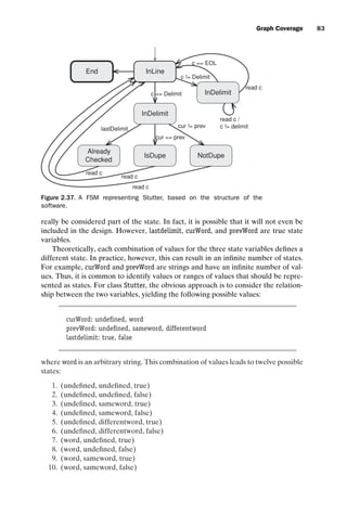
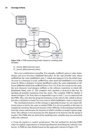
![introtest CUUS047-Ammann ISBN 9780521880381 November 8, 2007 17:13 Char Count= 0
Graph Coverage 85
End
read c /
c != delimit
c != EOL
BetweenWords InWord
EndWord
DupeFound NoDupe
read c /
c == delimit ||
c == EOL
read c /
c == delimit ||
c == EOL
read c /
c == EOF
read c /
c == EOF
nil /
prev == cur
nil /
prev == cur
read c /
c != delimit
c != EOL
Figure 2.39. A FSM representing Stutter, based on the specifications.
This FSM looks a lot like the FSM based on the code, and this is to be expected.
At the same time, FSMs based on specifications are usually cleaner and easier to
understand. If the software is designed well, this type of FSM should contain the
same information that UML state charts contain.
EXERCISES
Section 2.5.
1. Use the class Queue in Figure 2.40 for questions (a)–(f) below. The queue is
managed in the usual circular fashion.
Suppose we build a FSM where states are defined by the representation vari-
ables of Queue. That is, a state is a 4-tuple defined by the values for [elements,
size, front, back]. For example, the initial state has the value [[null, null], 0, 0,
0], and the state that results from pushing an object obj onto the queue in its
initial state is [[obj, null], 1, 0, 1].
(a) We do not actually care which specific objects are in the queue. Conse-
quently, there are really just four useful values for the variable elements.
Enumerate them.
(b) How many states are there?
(c) How many of these states are reachable?
(d) Show the reachable states in a drawing.
(e) Add edges for the enqueue() and dequeue() methods. (For this assign-
ment, ignore the exceptional returns, although you should observe that
when exceptional returns are taken, none of the instance variables are
modified.)
(f) Define a small test set that achieves edge coverage. Implement and exe-
cute this test set. You might find it helpful to write a method that shows
the internal variables at each call.](https://image.slidesharecdn.com/introductiontosoftwaretesting-221201191322-f16668ac/85/Introduction-to-Software-Testing-pdf-109-320.jpg)
![introtest CUUS047-Ammann ISBN 9780521880381 November 8, 2007 17:13 Char Count= 0
86 Coverage Criteria
public class Queue
{ // Overview: a Queue is a mutable, bounded FIFO data structure
// of fixed size (size is 2, for this exercise).
// A typical Queue is [], [o1], or [o1, o2], where neither o1 nor o2
// are ever null. Older elements are listed before newer ones.
private Object[] elements;
private int size, front, back;
private static final int capacity = 2;
public Queue ()
{
elements = new Object [capacity];
size = 0; front = 0; back = 0;
}
public void enqueue (Object o)
throws NullPointerException, IllegalStateException
{ // Modifies: this
// Effects: If argument is null throw NullPointerException
// else if this is full, throw IllegalStateException,
// else make o the newest element of this
if (o == null)
throw new NullPointerException (Queue.enqueue);
else if (size == capacity)
throw new IllegalStateException (Queue.enqueue);
else
{
size++;
elements [back] = o;
back = (back+1) % capacity;
}
}
public Object dequeue () throws IllegalStateException
{ // Modifies: this
// Effects: If queue is empty, throw IllegalStateException,
// else remove and return oldest element of this
if (size == 0)
throw new IllegalStateException (Queue.dequeue);
else
{
size--;
Object o = elements [ (front % capacity) ];
elements [front] = null;
front = (front+1) % capacity;
return o;
}
}
public boolean isEmpty() { return (size == 0); }
public boolean isFull() { return (size == capacity); }
public String toString()
{
String result = [;
for (int i = 0; i size; i++)
{
result += elements[ (front + i) % capacity ] . toString();
if (i size -1) {
result += , ;
}
}
result += ];
return result;
}
}
Figure 2.40. Class Queue for exercises.](https://image.slidesharecdn.com/introductiontosoftwaretesting-221201191322-f16668ac/85/Introduction-to-Software-Testing-pdf-110-320.jpg)
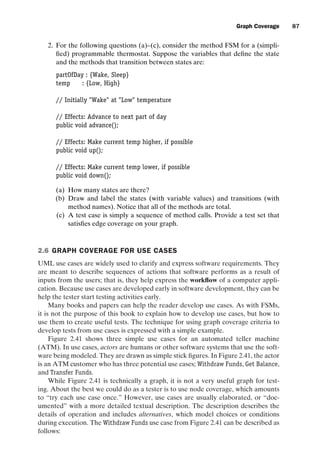
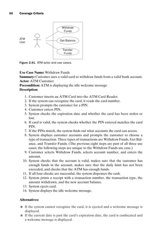
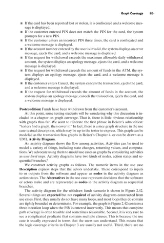
![introtest CUUS047-Ammann ISBN 9780521880381 November 8, 2007 17:13 Char Count= 0
90 Coverage Criteria
Insert ATM Card
Eject Card
[ card not
recognized ]
Enter PIN
Prompt for PIN
[ card
recognized ]
Confiscate Card
[ card
expired ]
[card not
lost ]
[ card not
expired ]
[card lost ]
Check PIN
[ invalid PIN ]
[ 3 tries ]
[ = 3 tries ]
[ valid PIN ]
Prompt for Transaction
Select Acct #
[ select
withdraw ]
[ select
balance or
transfer ]
[ invalid
account ]
[ insufficient
funds ]
[ daily amount
exceeded ]
[ ATM out
of funds ]
Eject Card
Dispense Cash
Print Receipt
Eject Card
Print Welcome
Message
[ valid
account ]
[ not
exceeded ]
[ sufficient
funds ]
[ not out
of funds ]
Figure 2.42. Activity graph for ATM withdraw funds.
obvious data definition-use pairs. This means that data flow coverage criteria are
not applicable.
The two criteria that are most obviously applicable to use case graphs are node
coverage and edge coverage. Test case values are derived from interpreting the
nodes and predicates as inputs to the software. One other criterion for use case
graphs is based on the notion of “scenarios.”
2.6.1 Use Case Scenarios
A use case scenario is an instance of, or a complete path through, a use case. A
scenario should make some sense semantically to the users and is often derived
when the use cases are constructed. If the use case graph is finite (as is usually the
case), then it is possible to list all possible scenarios. However, domain knowledge
can be used to reduce the number of scenarios that are useful or interesting from
either a modeling or test case perspective. Note that specified path coverage, defined
at the beginning of this chapter, is exactly what we want here. The set S for specified
path coverage is simply the set of all scenarios.
If the tester or requirements writer chooses all possible paths as scenarios, then
specified path coverage is equivalent to complete path coverage. The scenarios are
chosen by people and they depend on domain knowledge. Thus it is not guaranteed
that specified path coverage subsumes edge coverage or node coverage. That is, it
is possible to choose a set of scenarios that do not include every edge. This would
probably be a mistake, however. So, in practical terms, specified path coverage can
be expected to cover all edges.](https://image.slidesharecdn.com/introductiontosoftwaretesting-221201191322-f16668ac/85/Introduction-to-Software-Testing-pdf-114-320.jpg)
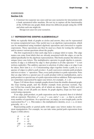
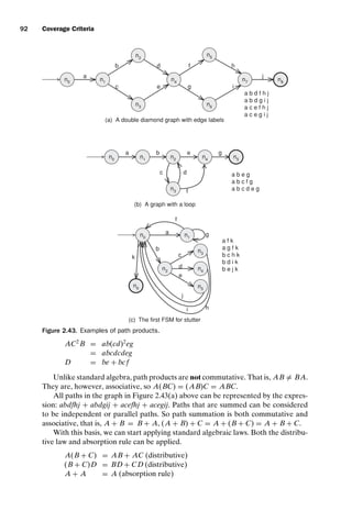

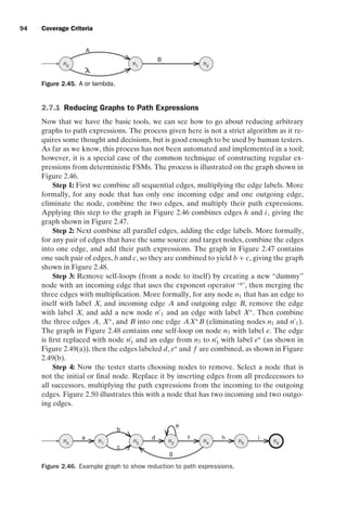
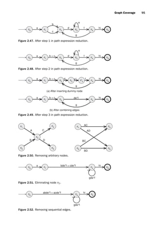
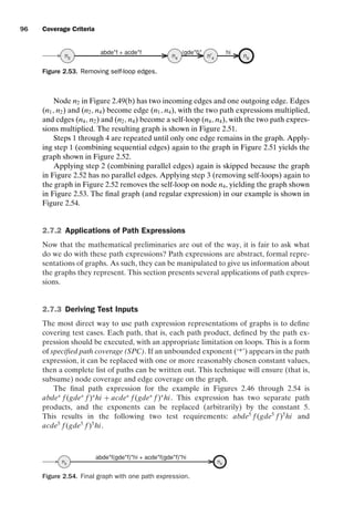
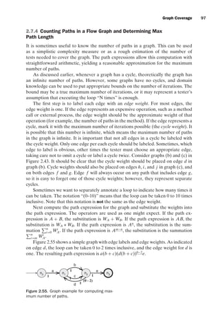
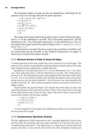
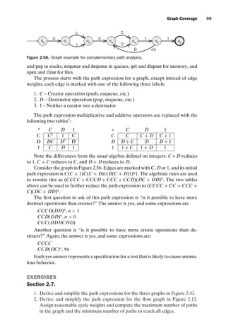
![introtest CUUS047-Ammann ISBN 9780521880381 November 8, 2007 17:13 Char Count= 0
100 Coverage Criteria
3. The graph in Figure 2.10 was used as an example for prime test paths. Add
appropriate edge labels to the graph, then derive and simplify the path expres-
sions. Next add edge weights of 1 for non-cycle edges and 5 for cycle edges.
Then compute the maximum number of paths in the graph and the minimum
number of paths to reach all edges. This graph has 25 prime paths. Briefly
discuss the number of prime paths with the maximum number of paths and
consider the effect of varying the cycle weight on the maximum number of
paths.
4. Section 2.5 presented four different versions of a FSM for Stutter. Derive and
simplify the path expressions for each of the four variations, then compute
the maximum number of paths and the minimum number of paths to reach
all edges in each. Discuss how the different numbers affect testing.
5. Perform complementary operations analysis on the graph in Figure 2.32. As-
sume complementary operators of open and close.
6. Derive and simplify the path expressions for the activity graph in Figure 2.42.
The only loop in that graph has a bound of 3 tries. Use that to compute the
maximum number of paths and the minimum number of paths to reach all
edges. Discuss the relationship between the scenarios for that graph and the
terms in the path expression.
7. Answer questions (a)–(c) for the graph defined by the following sets:
N = {1, 2, 3, 4, 5, 6, 7, 8, 9, 10}
N0 = {1}
Nf = {10}
E = {(1, 2, a), (2, 3, b), (2, 4, c), (3, 5, d), (4, 5, e), (5, 6, f ), (5, 7, g), (6, 6, h
(1 − 4)), (6, 10, i), (7, 8, j), (8, 8, k(0 − 3)), (8, 9,l), (9, 7, m(2 − 5)), (9, 10,
n)}
(a) Draw the graph.
(b) What is the maximum number of paths through the graph?
(c) What is the approximate minimum number of paths through the graph?
2.8 BIBLIOGRAPHIC NOTES
During the research for this book, one thing that became abundantly clear is that
this field has had a significant amount of parallel discovery of the same techniques by
people working independently. Some individuals have discovered various aspects of
the same technique, which was subsequently polished into very pretty test criteria.
Others have invented the same techniques, but based them on different types of
graphs or used different names. Thus, ascribing credit for software testing criteria is
a perilous task. We do our best, but claim only that the bibliographic notes in this
book are starting points for further study in the literature.
The research into covering graphs seems to have started with generating tests
from finite state machines (FSMs), which has a long and rich history. Some of the
earliest papers were in the 1970s [77, 164, 170, 232, 290]. The primary focus of most
of these papers was on using FSMs to generate tests for telecommunication systems
that were defined with standard finite automata, although much of the work per-
tained to general graphs. The control flow graph seems to have been invented (or
should it be termed “discovered”?) by Legard in 1975 [204]. In papers published](https://image.slidesharecdn.com/introductiontosoftwaretesting-221201191322-f16668ac/85/Introduction-to-Software-Testing-pdf-124-320.jpg)
![introtest CUUS047-Ammann ISBN 9780521880381 November 8, 2007 17:13 Char Count= 0
Graph Coverage 101
in 1975, Huang [170] suggested covering each edge in the FSM, and Howden [164]
suggested covering complete trips through the FSM, but without looping. In 1976,
McCabe [232] suggested the same idea on control flow graphs as the primary ap-
plication of his cyclomatic complexity metric. In 1976, Pimont and Rault [290] sug-
gested covering pairs of edges, using the term “switch cover.” In 1978, Chow [77]
suggested generating a spanning tree from the FSM and then basing test sequences
on paths through this tree. In 1991, Fujiwara et al. [130] extended Pimont and
Rault’s pairs of edges to arbitrary lengths, and used the term “n-switch” to refer
to a sequence of edges. He also attributed “1-switch,” or switch cover, to Chow and
called it the “W-method,” an inaccuracy that has been repeated in numerous pa-
pers. The idea of covering pairs of edges was rediscovered in the 1990s. The British
Computer Society Standard for Software Component Testing called it two-trip [317]
and Offutt et al. [272], called it transition-pair.
Other test generation methods based on FSMs include tour [251], the distin-
guished sequence method [137], and unique input-output method [307]. Their ob-
jectives are to detect output errors based on state transitions driven by inputs. FSM-
based test generation has been used to test a variety of applications including lex-
ical analyzers, real-time process control software, protocols, data processing, and
telephony. One early realization when developing this book is that the criteria for
covering FSMs are not substantially different from criteria for other graphs.
This book has introduced the explicit inclusion of node coverage requirements in
edge coverage requirements (the “up to” clause). This inclusion is not necessary for
typical control flow graphs, where, indeed, subsumption of node coverage by edge
coverage is often presented as a basic theorem, but it may be required for graphs
derived from other artifacts.
Several later papers focused on automatic test data generation to cover struc-
tural elements in the program [39, 41, 80, 101, 117, 166, 190, 191, 267, 295]. Much of
this work was based on the analysis techniques of symbolic evaluation [62, 83, 93,
101, 116, 164], and slicing [328, 339]. Some of these ideas are discussed in Chapter 6.
The problem of handling loops has plagued graph-based criteria from the begin-
ning. It seems obvious that we want to cover paths, but loops create infinite numbers
of paths. In Howden’s 1975 paper [164], he specifically addressed loops by cover-
ing complete paths “without looping,” and Chow’s 1978 suggestion to use spanning
trees was an explicit attempt to avoid having to execute loops [77]. Binder’s book
[33] used the technique from Chow’s paper, but changed the name to round trip,
which is the name used in this book.
Another early suggestion was based on testing loop free programs [66], which is
certainly interesting from a theoretical view, but not particularly practical.
White and Wiszniewski [348] suggested limiting the number of loops that need to
be executed based on specific patterns. Weyuker, Weiss, and Hamlet tried to choose
specific loops to test based on data definitions and uses [345].
The notion of subpath sets was developed by Offutt et al. [178, 265] to sup-
port inter-class path testing and is essentially equivalent to tours with detours as
presented here. The ideas of touring, sidetrips and detours were introduced by
Ammann, Offutt and Huang [17].
The earliest reference we have found on data flow testing was a technical report
in 1974 by Osterweil and Fosdick [282]. This technical report was followed by a 1976](https://image.slidesharecdn.com/introductiontosoftwaretesting-221201191322-f16668ac/85/Introduction-to-Software-Testing-pdf-125-320.jpg)
![introtest CUUS047-Ammann ISBN 9780521880381 November 8, 2007 17:13 Char Count= 0
102 Coverage Criteria
paper in ACM Computing Surveys [122], along with an almost simultaneous publi-
cation by Herman in the Australian Computer Journal [158]. The seminal data flow
analysis procedure (without reference to testing) was due to Allen and Cocke [13].
Other fundamental and theoretical references are by Laski and Korel in 1983
[201], who suggested executing paths from definitions to uses, Rapps and Weyuker
in 1985 [297], who defined criteria and introduced terms such as All-Defs and All-
Uses, and Frankl and Weyuker in 1988 [128]. These papers refined and clarified the
idea of data flow testing, and are the basis of the presentation in this text. Stated in
the language in this text, [128] requires direct tours for the All-du-Paths Coverage,
but allows sidetrips for All-Defs coverage and All-Uses coverage. This text allows
sidetrips (or not) for all of the data flow criteria. The pattern matching example
used in this text has been employed in the literature for decades; as far as we know,
Frankl and Weyuker [128] were the first to use the example for illustrating data flow
coverage.
Forman also suggested a way to detect data flow anomalies without running the
program [121].
Some detailed problems with data flow testing have been recurring. These in-
clude the application of data flow when paths between definitions and uses cannot
be executed [127], and handling pointers and arrays [267, 345].
The method of defining data flow criteria in terms of sets of du-paths is original
to this book, as is the explicit suggestion for best-effort eouring.
Many papers present empirical studies of various aspects of data flow testing.
One of the earliest was by Clarke, Podgurski, Richardson, and Zeil, who compared
some of the different criteria [82]. Comparisons with mutation testing (introduced
in Chapter 5) started with Mathur in 1991 [228], which was followed by Mathur and
Wong [230], Wong and Mathur [357], Offutt, Pan, Tewary, and Zhang [274], and
Frankl, Weiss, and Hu [125]. Comparisons of data flow with other test criteria have
been published by Frankl and Weiss [124], Hutchins, Foster, Goradia, and Ostrand
[172], and Frankl and Deng [123].
A number of tools have also been built by researchers to support data flow test-
ing. Most worked by taking a program and tests as inputs, and deciding whether
one or more data flow criteria have been satisfied (a recognizer). Frankl, Weiss, and
Weyuker built ASSET in the mid 1980s [126], Girgis and Woodward built a tool to
implement both data flow and mutation testing in the mid 1980s [134], and Laski
built STAD in the late 1980s [200]. Researchers at Bellcore developed the ATAC
data flow tool for C programs in the early 1990s [161, 162], and the first tool that
included a test data generator for data flow criteria was built by Offutt, Jin, and Pan
in the late 1990s [267].
Coupling was first discussed as a design metric by Constantine and Yourdon [88],
and its use for testing was introduced implicitly by Harrold, Soffa, and Rothermel
[152, 154] and explicitly by Jin and Offutt [178], who introduced the use of first-uses
and last-defs.
Kim, Hong, Cho, Bae, and Cha used a graph-based approach to generate tests
from UML state diagrams [186].
The USA’s Federal Aviation Authority (FAA) has recognized the increased
importance of modularity and integration testing by imposing requirements on
structural coverage analysis of software that “the analysis should confirm the data](https://image.slidesharecdn.com/introductiontosoftwaretesting-221201191322-f16668ac/85/Introduction-to-Software-Testing-pdf-126-320.jpg)
![introtest CUUS047-Ammann ISBN 9780521880381 November 8, 2007 17:13 Char Count= 0
Graph Coverage 103
coupling and control coupling between the code components” [305], p. 33, section
6.4.4.2.
Data flow testing has also been applied to integration testing by Harrold and
Soffa [154], Harrold and Rothermel [152], and Jin and Offutt [178]. This work
focused on class-level integration issues, but did not address inheritance or poly-
morphism. Data flow testing has been applied to inheritance and polymorphism in
object-oriented software by Alexander and Offutt [11, 10, 12], and Buy, Orso, and
Pezze [60, 281]. Gallagher and Offutt modeled classes as interacting state machines,
and tested concurrency and communication issues among them [132].
SCR was first discussed by Henninger [157], and its use in model checking and
testing was introduced by Atlee [20].
Constructing tests from UML diagrams is a more recent development, though
relatively straightforward. It was first suggested by Abdurazik and Offutt [2, 264],
and soon followed by Briand and Labiche [45].
The mechanisms for turning finite automata into regular expressions are stan-
dard fare in CS theory classes. As far as we know, Beizer [29] was the first to note
the utility of these transformations in the testing context.
NOTES
1 By way of example, typical control flow graphs have very few, if any, syntactically unreach-
able nodes, but call graphs, especially for object-oriented programs, often do.
2 Our mathematician readers might notice that this definition is constructive in that it defines
what is in the set TR, but does not actually bound the set. It is certainly our intention that
TR contains no other elements.
3 The reader might wonder why NOTFOUND fails to appear in the set use(2). The reason, as
explained in Section 2.3.2 is that the use is local.
4 The reader is cautioned that despite the names of the criteria, All-Defs and All-Uses are
not complementary criteria with respect to how they tread definitions and uses. Specifi-
cally, one does not arrive at All-Uses by replacing the notion of “def” with that of “use”
in All-Defs. The reader might find it helpful to note that while All-Defs focuses on defini-
tions, All-Uses focuses on def-use pairs. While one could argue that the naming convention
is misleading, and that a name such as “All-Pairs” might be preferable to All-Uses, the au-
thors elected to stick with the standard usage in the dataflow literature.
5 This is a bit of an overstatement, and, as usual, the culprit is infeasibility. Specifically, con-
sider a du-path with respect to variable x that can only be toured with a sidetrip. Further,
suppose that there are two possible sidetrips, one of which is def-clear with respect to x,
and one of which is not. The relevant test path from the All-du-Paths test set necessarily
tours the former sidetrip, where as the corresponding test path from the prime path test set
is free to tour the latter side trip. Our opinion is that in most situations it is reasonable for
the test engineer to ignore this special case and simply proceed with prime path coverage.
6 As in previous chapters, we explicitly leave out concurrency, so concurrent forks and joins
are not considered.
7 Mathematicians who have studied abstract algebra will recognize that these tables define
another algebra.](https://image.slidesharecdn.com/introductiontosoftwaretesting-221201191322-f16668ac/85/Introduction-to-Software-Testing-pdf-127-320.jpg)
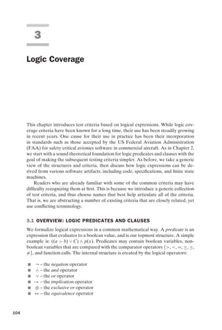
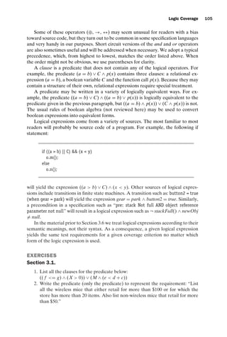
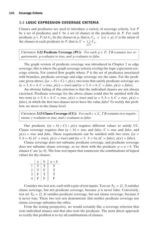
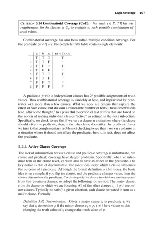
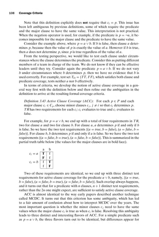
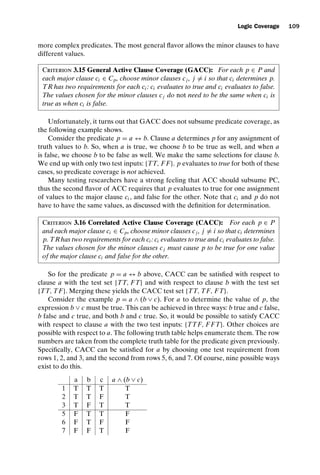
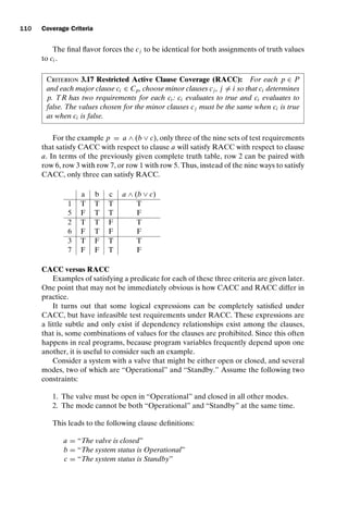
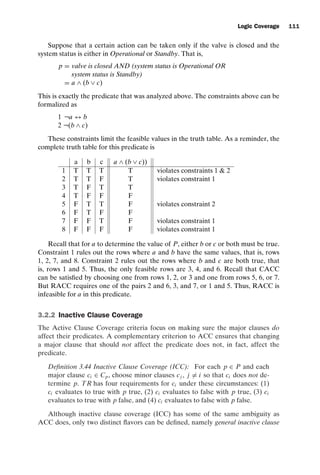
![introtest CUUS047-Ammann ISBN 9780521880381 November 8, 2007 17:13 Char Count= 0
112 Coverage Criteria
coverage (GICC) and restricted inactive clause coverage (RICC). The notion of
correlation is not relevant for Inactive Clause Coverage because ci cannot corre-
late with p since ci does not determine p. Also, predicate coverage is guaranteed,
subject to feasibility, in all flavors due to the structure of the definition.
The following example illustrates the value of the inactive clause coverage crite-
ria. Suppose you are testing the control software for a shutdown system in a reactor,
and the specification states that the status of a particular valve (open vs. closed) is
relevant to the reset operation in Normal mode, but not in Override mode. That is, the
reset should perform identically in Override mode when the valve is open and when
the valve is closed. The sceptical test engineer will want to test reset in Override mode
for both positions of the valve, since a reasonable implementation mistake would be
to take account the setting of the valve in all modes.
The formal versions of GICC and RICC are as follows.
Criterion 3.18 General Inactive Clause Coverage (GICC): For each p ∈ P and
each major clause ci ∈ Cp, choose minor clauses cj , j = i so that ci does not deter-
mine p. TRhas four requirements for ci under these circumstances: (1) ci evaluates
to true with p true, (2) ci evaluates to false with p true, (3) ci evaluates to true with
p false, and (4) ci evaluates to false with p false. The values chosen for the minor
clauses cj may vary amongst the four cases.
Criterion 3.19 Restricted Inactive Clause Coverage (RICC): For each p ∈ P
and each major clause ci ∈ Cp, choose minor clauses cj , j = i so that ci does not
determine p. TR has four requirements for ci under these circumstances: (1) ci
evaluates to true with p true, (2) ci evaluates to false with p true, (3) ci evaluates to
true with p false, and (4) ci evaluates to false with p false. The values chosen for
the minor clauses cj must be the same in cases (1) and (2), and the values chosen
for the minor clauses cj must also be the same in cases (3) and (4).
3.2.3 Infeasibility and Subsumption
A variety of technical issues complicate the Active Clause Coverage criteria. As with
many criteria, the most important is the issue of infeasibility. Infeasibility is often a
problem because clauses are sometimes related to one another. That is, choosing the
truth value for one clause may affect the truth value for another clause. Consider,
for example, a common loop structure, which assumes short circuit semantics:
while (i n a[i] != 0) {do something to a[i]}
The idea here is to avoid evaluating a[i] if i is out of range, and short circuit eval-
uation is not only assumed, but depended on. Clearly, it is not going to be possible
to develop a test case where i n is false and a[i] != 0 is true.
In principle, the issue of infeasibility for clause and predicate criteria is no differ-
ent from that for graph criteria. In both cases, the solution is to satisfy test require-
ments that are feasible, and then decide how to treat infeasible test requirements.](https://image.slidesharecdn.com/introductiontosoftwaretesting-221201191322-f16668ac/85/Introduction-to-Software-Testing-pdf-136-320.jpg)
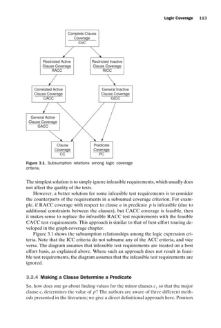
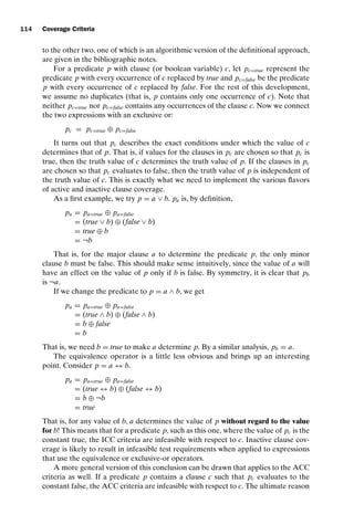
![introtest CUUS047-Ammann ISBN 9780521880381 November 8, 2007 17:13 Char Count= 0
116 Coverage Criteria
and they can be satisfied with the following values for the clauses:
a b c
p = true t t t
p = false t t f
To run the test cases, we need to refine these truth assignments to create values for
clauses a, b, and c. Suppose that clauses a, b, and c were defined in terms of Java
program variables as follows:
a x y, a relational expression for program variables x and y
b done, a primitive boolean value
c list.contains(str), for List and String objects
Thus, the complete expanded predicate is actually
p = (x y ∨ done) ∧ list.contains(str)
Then the following values for the program variables satisfy the test requirements
for predicate coverage.
a b c
p = true x=3 y=5 done = true list=[“Rat,” “Cat,” “Dog”] str = “Cat”
p = false x=0 y=7 done = true list=[“Red,” “White”] str = “Blue”
Note that the values for the program variables need not be the same in a par-
ticular test case if the goal is to set a clause to a particular value. For example,
clause a is true in both tests, even though program variables x and y have different
values.
Values to satisfy clause coverage were also shown in Section 3.2. Six test require-
ments are
TRCC = {a = true, a = false, b = true, b = false, c = true, c = false}
and they can be satisfied with the following values for the clauses (blank cells repre-
sent “don’t-care” values):
a b c
a = true t
a = false f
b = true t
b = false f
c = true t
c = false f
Refining the truth assignments to create values for program variables x, y, done, list,
and str is left as an exercise for the reader.
Before proceeding with the other criteria, we first choose values for minor
clauses to ensure that the major clauses will determine the value of p. We gave a](https://image.slidesharecdn.com/introductiontosoftwaretesting-221201191322-f16668ac/85/Introduction-to-Software-Testing-pdf-140-320.jpg)
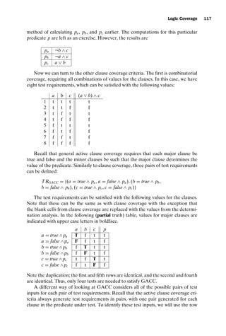
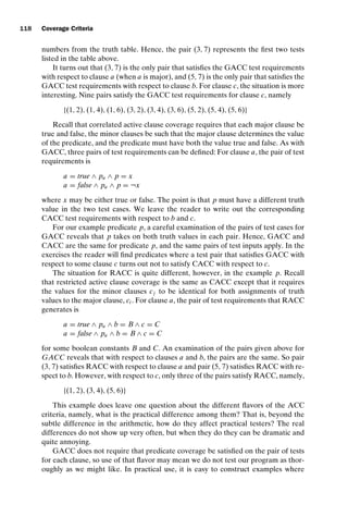
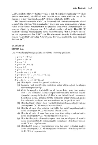
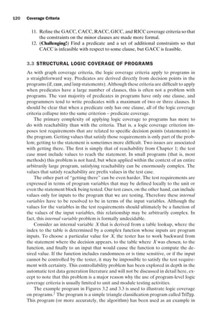
![introtest CUUS047-Ammann ISBN 9780521880381 November 8, 2007 17:13 Char Count= 0
Logic Coverage 121
1 // Jeff Offutt--Java version Feb 2003
2 // Classify triangles
3 import java.io.*;
4
5 class trityp
6 {
7 private static String[] triTypes = { , // Ignore 0.
8 scalene, isosceles, equilateral,
not a valid triangle};
9 private static String instructions = This is the ancient
TriTyp program.nEnter three integers that represent the
lengths of the sides of a triangle.nThe triangle will be
categorized as either scalene, isosceles, equilateraln
or invalid.n;
10
11 public static void main (String[] argv)
12 { // Driver program for trityp
13 int A, B, C;
14 int T;
15
16 System.out.println (instructions);
17 System.out.println (Enter side 1: );
18 A = getN();
19 System.out.println (Enter side 2: );
20 B = getN();
21 System.out.println (Enter side 3: );
22 C = getN();
23 T = Triang (A, B, C);
24
25 System.out.println (Result is: + triTypes[T]);
26 }
27
28 // ====================================
29 // The main triangle classification method
30 private static int Triang (int Side1, int Side2, int Side3)
31 {
32 int triOut;
33
34 // triOut is output from the routine:
35 // Triang = 1 if triangle is scalene
36 // Triang = 2 if triangle is isosceles
37 // Triang = 3 if triangle is equilateral
38 // Triang = 4 if not a triangle
39
40 // After a quick confirmation that it’s a valid
41 // triangle, detect any sides of equal length
42 if (Side1 = 0 || Side2 = 0 || Side3 = 0)
43 {
44 triOut = 4;
45 return (triOut);
46 }
47
48 triOut = 0;
49 if (Side1 == Side2)
50 triOut = triOut + 1;
51 if (Side1 == Side3)
52 triOut = triOut + 2;
53 if (Side2 == Side3)
54 triOut = triOut + 3;
55 if (triOut == 0)
56 { // Confirm it’s a valid triangle before declaring
57 // it to be scalene
58
Figure 3.2. TriTyp – Part A.](https://image.slidesharecdn.com/introductiontosoftwaretesting-221201191322-f16668ac/85/Introduction-to-Software-Testing-pdf-145-320.jpg)
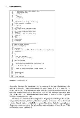
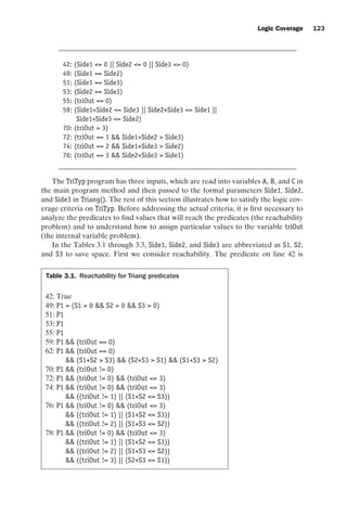
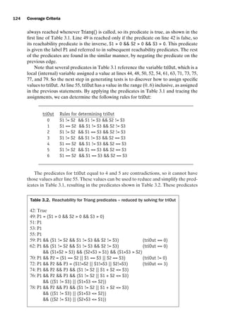
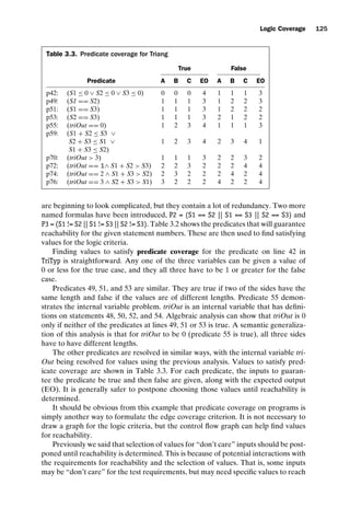
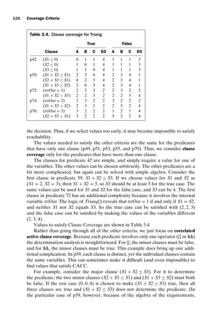
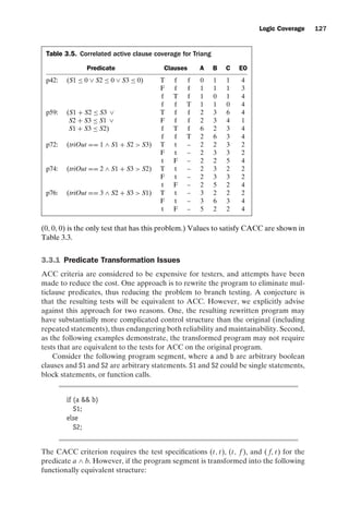
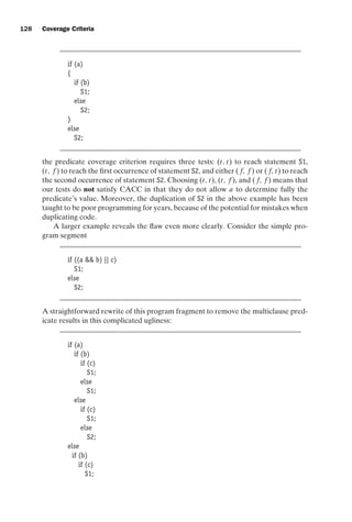
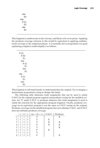
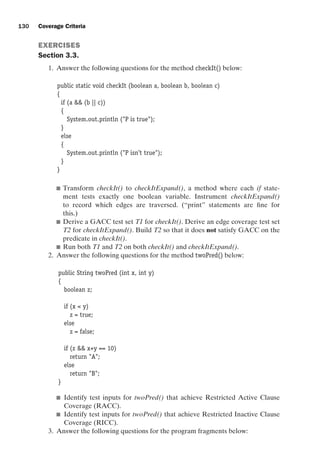
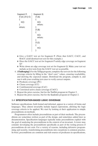
![introtest CUUS047-Ammann ISBN 9780521880381 November 8, 2007 17:13 Char Count= 0
132 Coverage Criteria
public static int cal (int month1, int day1, int month2,
int day2, int year)
{
//***********************************************************
// Calculate the number of Days between the two given days in
// the same year.
// preconditions : day1 and day2 must be in same year
// 1 = month1, month2 = 12
// 1 = day1, day2 = 31
// month1 = month2
// The range for year: 1 ... 10000
//***********************************************************
int numDays;
if (month2 == month1) // in the same month
numDays = day2 - day1;
else
{
// Skip month 0.
int daysIn[] = {0, 31, 0, 31, 30, 31, 30, 31, 31, 30, 31, 30, 31};
// Are we in a leap year?
int m4 = year % 4;
int m100 = year % 100;
int m400 = year % 400;
if ((m4 != 0) || ((m100 == 0) (m400 != 0)))
daysIn[2] = 28;
else
daysIn[2] = 29;
// start with days in the two months
numDays = day2 + (daysIn[month1] - day1);
// add the days in the intervening months
for (int i = month1 + 1; i = month2-1; i++)
numDays = daysIn[i] + numDays;
}
return (numDays);
}
Figure 3.4. Calendar method.
and so we focus on them here. Of course, other specification constructs, such as
postconditions and invariants, also are rich sources of complex predicates.
Consider the cal method in Figure 3.4. The method lists explicit preconditions in
natural language. These can be translated into predicate form as follows:
month1 = 1 ∧ month1 = 12 ∧ month2 = 1 ∧ month2 = 12 ∧ month1 = month2
∧ day1 = 1 ∧ day1 = 31 ∧ day2 = 1 ∧ day2 = 31 ∧ year = 1 ∧ year = 10000
The comment about day1 and day2 being in the same year can be safely ig-
nored, because that prerequisite is enforced syntactically by the fact that only one
parameter appears for year. It is probably also clear that these preconditions are not
complete. Specifically, a day of 31 is valid only for some months. This requirement
should be reflected in the specifications or in the program.
This predicate has a very simple structure. It has eleven clauses (which sounds
like a lot!) but the only logical operator is “and.” Satisfying predicate coverage
for cal() is simple – all clauses need to be true for the true case and at least one
clause needs to be false for the false case. So (month1 = 4, month2 = 4, day1 = 12,
day2 = 30, year = 1961) satisfies the true case, and the false case is satisfied by vi-
olating the clause month1 = month2, with (month1 = 6, month2 = 4, day1 = 12,
day2 = 30, year = 1961). Clause coverage requires all clauses to be true and false.](https://image.slidesharecdn.com/introductiontosoftwaretesting-221201191322-f16668ac/85/Introduction-to-Software-Testing-pdf-156-320.jpg)
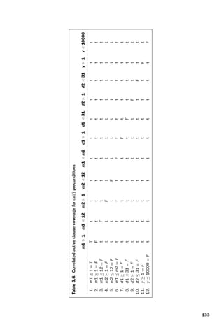
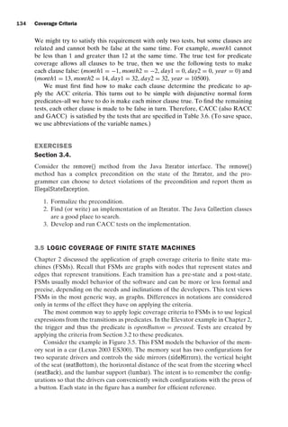
![introtest CUUS047-Ammann ISBN 9780521880381 November 8, 2007 17:13 Char Count= 0
Logic Coverage 135
Press seatBottom button
[ Ignition = on]
2
Driver 2
Configuration
3
Modified
Configuration
4
New Configuration
Driver1
5
New Configuration
Driver2
1
Driver 1
Configuration
Button2 [ Gear = Park OR
Ignition = off ]
Button1 [ Gear = Park OR
Ignition = off ]
ignition = off
seatBack button
[ Ignition = on]
Press lumbar button
[ Ignition = on]
Press sideMirrors button
[ Ignition = on]
seatBack button
[ Ignition = on]
seatBottom button
[ Ignition = on]
lumbar button
[ Ignition = on]
sideMirrors button
[ Ignition = on]
ignition = off
Reset and Button1
[ Ignition = on]
Reset and Button2
[ Ignition = on]
seatBack button
[ Ignition = on]
lumbar button
[ Ignition = on]
seatBottom button
[ Ignition = on]
sideMirrors button
[ Ignition = on]
seatBack button
[ Ignition = on]
lumbar button
[ Ignition = on]
seatBottom button
[ Ignition = on]
sideMirrors button
[ Ignition = on]
Button2 [ Gear = Park OR
Ignition = off ]
Button1 [ Gear = Park OR
Ignition = off ]
Figure 3.5. FSM for a memory car seat – Lexus 2003 ES300.
The initial state of the FSM is whichever configuration it was in when the system
was last shut down, either Driver 1, Driver 2, or Modified Configuration. The drivers
can modify the configuration by changing one of the four controls; changing the
side mirrors, moving the seat backwards or forwards, raising or lowering the seat, or
modifying the lumbar support (triggering events). These controls work only if the
ignition is on (a guard). The driver can also change to the other configuration by
pressing either Button1 or Button2 when the ignition is on. In these cases, the guards
allow the configuration to be changed only if the Gear is in Park or the ignition is off.
These are safety constraints, because it would be dangerous to allow the driver’s seat
to go flying around when the car is moving.
When the driver changes one of the controls, the memory seat is put into the
modified configuration state. The new state can be saved by simultaneously pressing
the Reset button and either Button1 or Button2 when the ignition is on. The new
configuration is saved permanently when the ignition is turned off.
This type of FSM provides an effective model for testing software, although sev-
eral issues must be understood and dealt with when creating predicates and then test
values. Guards are not always explicitly listed as conjuncts, but they are conjuncts in
effect and so should be combined with the triggers using the AND operator. In some
specification languages, most notably SCR, the triggers actually imply two values.
In SCR, if an event is labeled as triggering, it means that the value of the resulting
expression must explicitly change. This implies two values, a before value and an](https://image.slidesharecdn.com/introductiontosoftwaretesting-221201191322-f16668ac/85/Introduction-to-Software-Testing-pdf-159-320.jpg)
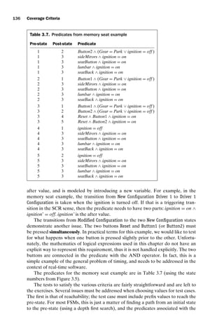
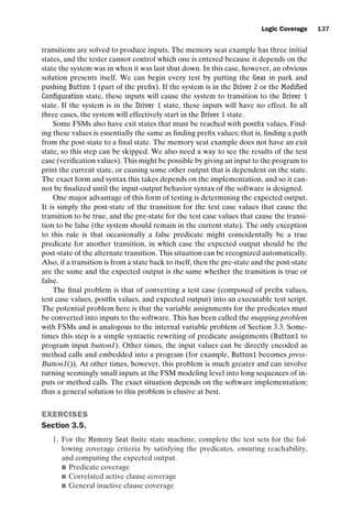
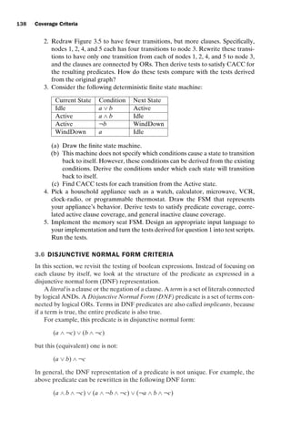
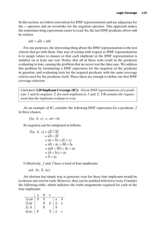
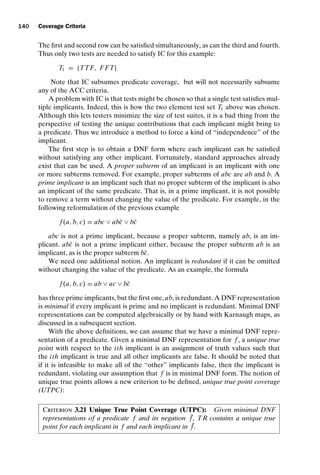
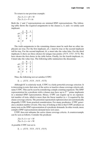
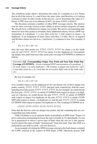
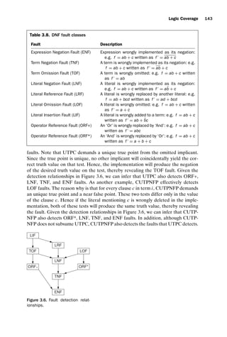
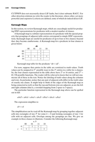
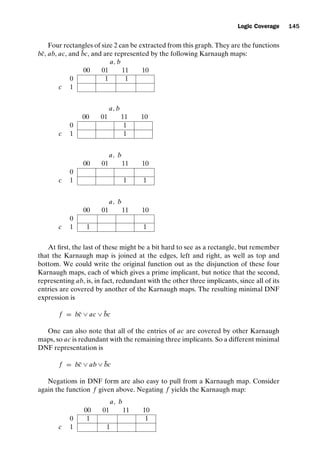
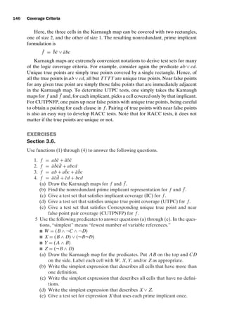
![introtest CUUS047-Ammann ISBN 9780521880381 November 8, 2007 17:13 Char Count= 0
Logic Coverage 147
6 Develop a counterexample to show that CUTPNFP does not subsume UPIC.
Hint: You might wish to start with the expression given in the text, f = ab +
cd.
3.7 BIBLIOGRAPHIC NOTES
The active clause criteria seem to have their beginnings in Myers’ 1979 book [249]. A
more accessible paper is by Zhu [367]. He defined decision and condition coverage,
which Chilenski and Miller later used as a conceptual basis for MCDC [73, 305].
The definitions as originally given correspond to GACC in this book and did not
address whether minor clauses had to have the same value for both values of the
major clause. Chilenski also emphasized that the abbreviation should be “MCDC,”
not “MC/DC,” and he has never put the ‘/’ in the middle [72]. Most members of
the aviation community interpreted MCDC to mean that the values of the minor
clauses had to be the same, an interpretation that is called “unique-cause MCDC”
[72]. Unique-cause MCDC corresponds to our RACC. More recently, the FAA
has accepted the view that the minor clauses can differ, which is called “mask-
ing MCDC” [74]. Masking MCDC corresponds to our CACC. Our previous paper
[17] clarified the definitions in the form used in this book and introduced the term
“CACC.”
The inactive clause criteria are adapted from the RC/DC method of Vilkomir
and Bowen [332].
The result that the internal variable problem is formally undecidable is from Of-
futt’s PhD dissertation [101, 262]. The problem is of primary importance in the au-
tomatic test data generation literature [36, 39, 101, 102, 150, 176, 179, 190, 191, 243,
295, 267].
Jasper et al. presented techniques for generating tests to satisfy MCDC [177].
They took the definition of MCDC from Chilenski and Miller’s paper with the “de-
fault” interpretation that the minor clauses must be the same for both values of the
major clauses. They went on to modify the interpretation so that if two clauses are
coupled, which implies it is impossible to satisfy determination for both, the two
clauses are allowed to have different values for the minor clauses. The fact that
different values are allowed only when clauses are coupled puts their interpretation
of MCDC between the RACC and CACC of this book.
Weyuker, Goradia, and Singh presented techniques for generating test data for
software specifications that are limited to boolean variables [342]. The techniques
were compared in terms of the ability of the resulting test cases to kill mutants
(introduced in Chapter 5) [99, 101]. The results were that their technique, which
is closely related to MCDC, performed better than any of the other techniques.
Weyuker et al. incorporated syntax as well as meaning into their criteria. They pre-
sented a notion called meaningful impact, which is related to the notion of determi-
nation, but which has a syntactic basis rather than a semantic one.
Kuhn investigated methods for generating tests to satisfy various decision-based
criteria, including MCDC tests [194]. He used the definition from Chilenski and
Miller [73, 305], and proposed the boolean derivative to satisfy MCDC. In effect,
this interpreted MCDC in such a way to match CACC.](https://image.slidesharecdn.com/introductiontosoftwaretesting-221201191322-f16668ac/85/Introduction-to-Software-Testing-pdf-171-320.jpg)
![introtest CUUS047-Ammann ISBN 9780521880381 November 8, 2007 17:13 Char Count= 0
148 Coverage Criteria
Dupuy and Leveson’s 2000 paper evaluated MCDC experimentally [108]. They
presented results from an empirical study that compared pure functional testing with
functional testing augmented by MCDC. The experiment was performed during the
testing of the attitude control software for the HETE-2 (High Energy Transient
Explorer) scientific satellite. The definition of MCDC from their paper is the tradi-
tional definition given in the FAA report and Chilenski and Miller’s paper: “Every
point of entry and exit in the program has been invoked at least once, every condi-
tion in a decision in the program has taken on all possible outcomes at least once,
and each condition has been shown to affect that decision outcome independently.
A condition is shown to affect a decision’s outcome independently by varying just
that decision while holding fixed all other possible conditions.”
Note the misstatement in last line: “varying just that decision” should be “vary-
ing just that condition.” This does not say that the decision has a different value
when the condition’s value changes. “Holding fixed” can be assumed to imply that
the minor clauses cannot change with different values for the major clause (that is,
RACC, not CACC).
The full predicate method of Offutt, Liu, Abdurazik and Ammann [272] explic-
itly relaxes the requirement that the major clauses have the same value as the pred-
icate. This is equivalent to CACC and almost the same as masking MCDC.
Jones and Harrold have developed a method for reducing the regression tests
that were developed to satisfy MCDC [180]. They defined MCDC as follows:
“MC/DC is a stricter form of decision (or branch) coverage. . . . MC/DC requires
that each condition in a decision be shown by execution to independently affect the
outcome of the decision.” This is taken directly from Chilenski and Miller’s original
paper, and their interpretation of the definition is the same as CACC.
SCR was first discussed by Henninger [157] and its use in model checking and
testing was introduced by Atlee [20, 21].
The method of determining pc given in this book uses the boolean derivative
developed by Akers [6]. Both Chilenski and Richey [74] and Kuhn [194] applied
Akers’s derivative to exactly the problem given in this chapter. The other methods
are the pairs table method of Chilenski and Miller and the tree method, indepen-
dently discovered by Chilenski and Richey [74] and Offutt et al. [272]. The tree
method implements the boolean derivative method in a procedural way.
Ordered binary decision diagrams (OBDDs) offer another way of determining
pc. In particular, consider any OBDD in which clause c is ordered last. Then any
path through the OBDD that reaches a node labeled c (there will be exactly zero,
one, or two such nodes) is, in fact, an assignment of values to the other variables
so that c determines p. Continuing the path on to the constants T and F yields a
pair of tests satisfying RACC with respect to c. Selecting two different paths that
reach the same node labeled c, and then extending each so that one reaches T and
the other reaches F yields a pair of tests that satisfy CACC, but not RACC, with
respect to c. Finally, if two nodes are labeled c, then it is possible to satisfy GACC
but not CACC with respect to c: Select paths to each of the two nodes labeled c,
extend one path by choosing c true, and the other by choosing c false. Both paths will
necessarily end up in the same node, namely, either T or F. ICC tests with respect
to c can be derived by considering paths to T and F in the OBDD where the paths](https://image.slidesharecdn.com/introductiontosoftwaretesting-221201191322-f16668ac/85/Introduction-to-Software-Testing-pdf-172-320.jpg)
![introtest CUUS047-Ammann ISBN 9780521880381 November 8, 2007 17:13 Char Count= 0
Logic Coverage 149
do not include variable c. The attractive aspect of using OBDDs to derive ACC or
ICC tests is that a variety of existing tools can handle a relatively large number of
clauses. The unattractive aspect is that for a predicate with N clauses, N different
OBDDs for a given function are required, since the clause being attended to needs
to be the last in the ordering. To the knowledge of the authors, the use of OBDDs
to derive ACC or ICC tests does not appear in the literature.
Beizer’s book [29] includes a chapter on DNF testing, including a variant of IC
coverage for f , but not ¯
f , and an extensive development of Karnaugh maps. We
do not address criteria defined predicates expressed in conjunctive normal form
(CNF). The reason is that every DNF coverage criteria has a dual in CNF. Kuhn
[194] developed the first fault detection relations; this work was greatly expanded
by Yu, Lau, and Chen, who developed much of the key material relating DNF cov-
erage criteria to fault detecting ability. Two good papers to begin study of this
topic are by Chen and Lau [63], which develops a variety of coverage criteria, in-
cluding CUTPNFP, and Lau and Yu [202], which is the source for the fault class
hierarchy shown in Figure 3.6. In personal communications, Greg Williams and
Gary Kaminski provided the authors with valuable assistance in organizing and ex-
panding the DNF fault detection material. Greg Williams also developed the coun-
terexample to show that UTPC and the ACC criteria do not share a subsumption
relation.
NOTES
1 In practice, this “thought” turned out to be the collective effort of many researchers, who
published dozens of papers over a period of several decades.
2 Old hands at testing may recognize and even be tired of the triangle example. It is used
as a teaching tool for the same reasons it has staying power in the literature: it’s a familiar
problem; the control structure is interesting enough to illustrate most issues; and it does
not use language features that make this analysis really hard, such as loops and indirect
references. This version of TriTyp is a bit overly complicated, but that does help illustrate
the concepts.
3 The notion of mutation operators developed in the Chapter 5 is closely related to the notion
of fault classes presented here.](https://image.slidesharecdn.com/introductiontosoftwaretesting-221201191322-f16668ac/85/Introduction-to-Software-Testing-pdf-173-320.jpg)
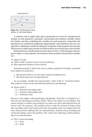
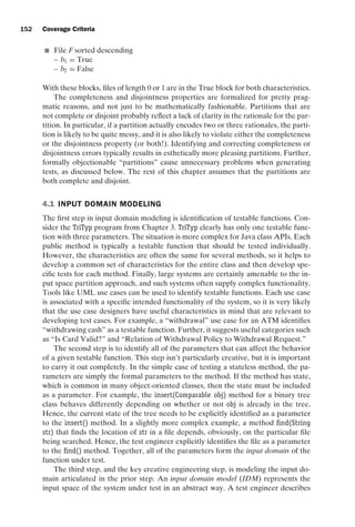
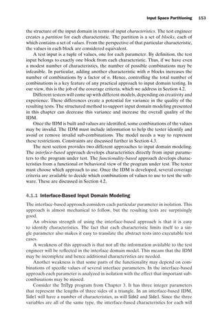
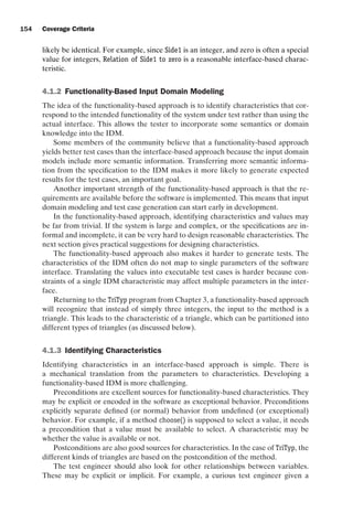
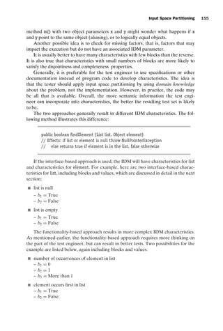
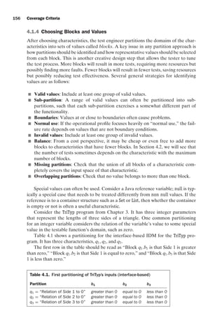
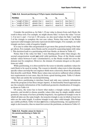
![introtest CUUS047-Ammann ISBN 9780521880381 November 8, 2007 17:13 Char Count= 0
Input Space Partitioning 159
Table 4.6. Possible values for blocks in geometric
partitioning in Table 4.5.
Param b1 b2 b3 b4
Triangle (4, 5, 6) (3, 3, 4) (3, 3, 3) (3, 4, 8)
characteristics and their blocks, it is time to choose which combinations of values to
test with and identify constraints among the blocks.
EXERCISES
Section 4.1.
1. Answer the following questions for the method search() below:
public static int search (List list, Object element)
// Effects: if list or element is null throw NullPointerException
// else if element is in the list, return an index
// of element in the list; else return -1
// for example, search ([3,3,1], 3) = either 0 or 1
// search ([1,7,5], 2) = -1
Base your answer on the following characteristic partitioning:
Characteristic: Location of element in list
Block 1: element is first entry in list
Block 2: element is last entry in list
Block 3: element is in some position other than first or last
(a) “Location of element in list” fails the disjointness property. Give an ex-
ample that illustrates this.
(b) “Location of element in list” fails the completeness property. Give an
example that illustrates this.
(c) Supply one or more new partitions that capture the intent of “Loca-
tion of e in list” but do not suffer from completeness or disjointness
problems.
2. Derive input space partitioning tests for the GenericStack class with the fol-
lowing method signatures:
public GenericStack ();
public void Push (Object X);
public Object Pop ();
public boolean IsEmt ();
Assume the usual semantics for the stack. Try to keep your partitioning sim-
ple, choose a small number of partitions and blocks.
(a) Define characteristics of inputs
(b) Partition the characteristics into blocks
(c) Define values for the blocks](https://image.slidesharecdn.com/introductiontosoftwaretesting-221201191322-f16668ac/85/Introduction-to-Software-Testing-pdf-183-320.jpg)
![introtest CUUS047-Ammann ISBN 9780521880381 November 8, 2007 17:13 Char Count= 0
160 Coverage Criteria
4.2 COMBINATION STRATEGIES CRITERIA
The above description ignores an important question: “How should we consider
multiple partitions at the same time?” This is the same as asking “What combination
of blocks should we choose values from?” For example, we might wish to require
a test case that satisfies block 1 from q2 and block 3 from q3. The most obvious
choice is to choose all combinations. However, just like Combinatorial Coverage
from previous chapters, using all combinations will be impractical when more than
2 or 3 partitions are defined.
Criterion 4.23 All Combinations Coverage (ACoC): All combinations of blocks
from all characteristics must be used.
For example, if we have three partitions with blocks [A, B], [1, 2, 3], and [x, y],
then ACoC will need the following twelve tests:
(A, 1, x) (B, 1, x)
(A, 1, y) (B, 1, y)
(A, 2, x) (B, 2, x)
(A, 2, y) (B, 2, y)
(A, 3, x) (B, 3, x)
(A, 3, y) (B, 3, y)
A test suite that satisfies ACoC will have a unique test for each combination of
blocks for each partition. The number of tests will be the product of the number of
blocks for each partition:
Q
i=1(Bi ).
If we use a four block partition similar to q2 for each of the three sides of the
triangle, ACoC requires 4 ∗ 4 ∗ 4 = 64 tests.
This is almost certainly more testing than is necessary, and will usually be eco-
nomically impractical as well. Thus, as with paths and truth tables before, we must
use some sort of coverage criterion to choose which combinations of blocks to pick
values from.
The first, fundamental assumption is that different choices of values from the
same block are equivalent from a testing perspective. That is, we need to take only
one value from each block. Several combination strategies exist, which result in a
collection of useful criteria. These combination strategies are illustrated with the
TriTyp example, using the second categorization given in Table 4.2 and the values
from Table 4.3.
The first combination strategy criterion is fairly straightforward and simply re-
quires that we try each choice at least once.
Criterion 4.24 Each Choice Coverage (ECC): One value from each block for
each characteristic must be used in at least one test case.
Given the above example of three partitions with blocks [A, B], [1, 2, 3], and
[x, y], ECC can be satisfied in many ways, including the three tests (A, 1, x), (B, 2, y),
and (A, 3, x).
Assume the program under test has Qparameters q1, q2, . . . , qQ, and each param-
eter qi has Bi blocks. Then a test suite that satisfies ECC will have at least MaxQ
i=1 Bi](https://image.slidesharecdn.com/introductiontosoftwaretesting-221201191322-f16668ac/85/Introduction-to-Software-Testing-pdf-184-320.jpg)
![introtest CUUS047-Ammann ISBN 9780521880381 November 8, 2007 17:13 Char Count= 0
Input Space Partitioning 161
values. The maximum number of blocks for the partitions for TriTyp is four, thus
ECC requires at least four tests.
This criterion can be satisfied by choosing the tests {(2, 2, 2), (1, 1, 1), (0, 0, 0),
(−1, −1, −1)} from Table 4.3. It does not take much thought to conclude that these
are not very effective tests for this program. ECC leaves a lot of flexibility to the
tester in terms of how to combine the test values, so it can be called a relatively
“weak” criterion.
The weakness of ECC can be expressed as not requiring values to be combined
with other values. A natural next step is to require explicit combinations of values,
called pair-wise.
Criterion 4.25 Pair-Wise Coverage (PWC): A value from each block for each
characteristic must be combined with a value from every block for each other
characteristic.
Given the above example of three partitions with blocks [A, B], [1, 2, 3], and
[x, y], then PWC will need sixteen tests to cover the following combinations:
(A, 1) (B, 1) (1, x)
(A, 2) (B, 2) (1, y)
(A, 3) (B, 3) (2, x)
(A, x) (B, x) (2, y)
(A, y) (B, y) (3, x)
(3, y)
PWC allows the same test case to cover more than one unique pair of values. So
the above combinations can be combined in several ways, including:
(A, 1, x) (B, 1, y)
(A, 2, x) (B, 2, y)
(A, 3, x) (B, 3, y)
(A, –, y) (B, –, x)
The tests with ‘–’ mean that any block can be used.
A test suite that satisfies PWC will pair each value with each other value or have
at least (MaxQ
i=1 Bi )2
values. Each characteristic in TriTyp (Table 4.3) has four blocks;
so at least 16 tests are required.
Several algorithms to satisfy PWC have been published and appropriate refer-
ences are provided in the bibliography section of the chapter.
A natural extension to PWC is to require t values instead of pairs.
Criterion 4.26 T-Wise Coverage (TWC): A value from each block for each group
of t characteristics must be combined.
If the value for T is chosen to be the number of partitions, Q, then TWC is
equivalent to all combinations. A test suite that satisfies TWC will have at least
(Max
q
i=1 Bi )t
values. TWC is expensive in terms of the number of test cases, and
experience suggests going beyond pair-wise (that is, t = 2) does not help much.](https://image.slidesharecdn.com/introductiontosoftwaretesting-221201191322-f16668ac/85/Introduction-to-Software-Testing-pdf-185-320.jpg)
![introtest CUUS047-Ammann ISBN 9780521880381 November 8, 2007 17:13 Char Count= 0
162 Coverage Criteria
Both PWC and TWC combine values “blindly,” without regard for which values
are being combined. The next criterion strengthens ECC in a different way by bring-
ing in a small but crucial piece of domain knowledge of the program; asking what is
the most “important” block for each partition. This block is called the base choice.
Criterion 4.27 Base Choice Coverage (BCC): A base choice block is chosen for
each characteristic, and a base test is formed by using the base choice for each char-
acteristic. Subsequent tests are chosen by holding all but one base choice constant
and using each non-base choice in each other characteristic.
Given the above example of three partitions with blocks [A, B], [1, 2, 3], and
[x, y], suppose base choice blocks are ‘A’, ‘1’ and ‘x’. Then the base choice test is
(A, 1, x), and the following additional tests would need to be used:
(B, 1, x)
(A, 2, x)
(A, 3, x)
(A, 1, y)
A test suite that satisfies BCC will have one base test, plus one test for each re-
maining block for each partition. This is a total of 1 +
Q
i=1(Bi − 1). Each parameter
for TriTyp has four blocks, thus BCC requires 1 + 3 + 3 + 3 tests.
The base choice can be the simplest, the smallest, the first in some ordering, or
the most likely from an end-user point of view. Combining more than one invalid
value is usually not useful because the software often recognizes one value and neg-
ative effects of the others are masked. Which blocks are chosen for the base choices
becomes a crucial step in test design that can greatly impact the resulting test. It is
important that the tester document the strategy that was used so that further testing
can reevaluate those decisions.
Following the strategy of choosing the most likely block for TriTyp, we chose
“greater than 1” from Table 4.2 as the base choice block. Using the values from
Table 4.3 gives the base test as (2, 2, 2). The remaining tests are created by varying
each one of these in turn: {(2, 2, 1), (2, 2, 0), (2, 2, −1), (2, 1, 2), (2, 0, 2), (2, −1, 2),
(1, 2, 2), (0, 2, 2), (−1, 2, 2) }.
Sometimes the tester may have trouble choosing a single base choice and may
decide that multiple base choices are needed. This is formulated as follows:
Criterion 4.28 Multiple Base Choices (MBCC): At least one, and possibly more,
base choice blocks are chosen for each characteristic, and base tests are formed by
using each base choice for each characteristic at least once. Subsequent tests are
chosen by holding all but one base choice constant for each base test and using
each non-base choice in each other characteristic.
Assuming mi base choices for each characteristic and a total of M base tests,
MBCC requires M +
Q
i=1(M ∗ (Bi − mi )) tests.
For example, we may choose to include two base choices for side 1 in TriTyp,
“greater than 1” and “equal to 1.” This would result in the two base tests (2, 2, 2)
and (1, 2, 2). The formula above is thus evaluated with M = 2, m1 = 2, and](https://image.slidesharecdn.com/introductiontosoftwaretesting-221201191322-f16668ac/85/Introduction-to-Software-Testing-pdf-186-320.jpg)
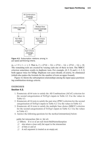
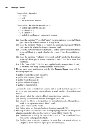
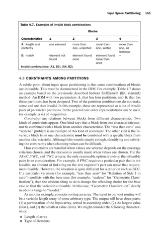
![introtest CUUS047-Ammann ISBN 9780521880381 November 8, 2007 17:13 Char Count= 0
166 Coverage Criteria
Max value
Min value
Position of max value
Position of min value
These characteristics can, in turn, reasonably result in the partitioning summa-
rized as follows:
Length {0, 1, 2. .100, 101. .MAXINT}
Type {int, char, string, other}
Max {≤ 0, 1, 1, ‘a’, ‘Z’, ‘b’, . . . , ‘Y’, blank, nonblank}
Min { · · · }
Max pos {1, 2..Length-1, Length}
Min pos {1, 2..Length-1, Length}
The discerning reader will of course notice that not all combinations are possible.
For example, if Length = 0, then nothing else matters. Also, some of the Max and
Min values are available only if Type = int, and others if Type = char.
4.4 BIBLIOGRAPHIC NOTES
In the research literature, several testing methods have been described that are
generally based on the model that the input space of the test object should be
divided into subsets, with the assumption that all inputs in the same subset cause
similar behavior. These are collectively called partition testing and include equiva-
lence partitioning [249], boundary value analysis [249], category partition [283], and
domain testing [29]. An extensive survey with examples was published by Grindal
et al. [143].
The derivation of partitions and values started with Balcer, Hasling, and Os-
trand’s category partition method in 1988 [23, 283]. An alternate visualization is
that of classification trees introduced by Grochtman, Grimm, and Wegener in 1993
[145, 146]. Classification trees organize the input space partitioning information into
a tree structure. The first level nodes are the parameters and environment vari-
ables (characteristics); they may be recursively broken into sub-categories. Blocks
appear as leaves in the tree and combinations are chosen by selecting among the
leaves.
Chen et al. empirically identified common mistakes that testers made during in-
put parameter-modeling [64]. Many of the concepts on input domain modeling in
this chapter come from Grindal’s PhD work [140, 142, 144]. Both Cohen et al. [84]
and Yin et al. [363] suggest functionality oriented approaches to input parameter
modeling. Functionality-oriented input parameter modeling was also implicitly used
by Grindal et al. [141]. Two other IDM-related methods are Classification Trees
[145] and a UML activity diagram based method [65]. Beizer [29], Malaiya [222],
and Chen et al. [64] also address the problem of characteristic selection.
Grindal published an analytical/empirical comparison of different constraint-
handling mechanisms [144].
Stocks and Carrington [320] provided a formal notion of specification-based test-
ing that encompasses most approaches to input space partition testing. In particular,](https://image.slidesharecdn.com/introductiontosoftwaretesting-221201191322-f16668ac/85/Introduction-to-Software-Testing-pdf-190-320.jpg)
![introtest CUUS047-Ammann ISBN 9780521880381 November 8, 2007 17:13 Char Count= 0
Input Space Partitioning 167
they addressed the problem of refining test frames (which we simply and informally
call test requirements in this book) to test cases.
The each choice and base choice criteria were introduced by Ammann and
Offutt in 1994 [16]. Cohen et al. [84] indicated that valid and invalid parameter val-
ues should be treated differently with respect to coverage. Valid values lie within
the bounds of normal operation of the test object, and invalid values lie outside
the normal operating range. Invalid values often result in an error message and the
execution terminates. To avoid one invalid value masking another, Cohen et al. sug-
gested that only one invalid value should be included in each test case.
Burroughs et al. [58] and Cohen et al. [84, 85, 86] suggested the heuristic pair-
wise coverage as part of the Automatic Efficient Test Generator (AETG). AETG
also includes a variation on the base choice combination criterion. In AETG’s ver-
sion, called “default testing,” the tester varies the values of one characteristic at a
time while the other characteristics contain some default value. The term “default
testing” was also used by Burr and Young [57], who described yet another varia-
tion of the base choices. In their version, all characteristics except one contain the
default value, and the remaining characteristics contain a maximum or a minimum
value. This variant will not necessarily satisfy “each choice coverage.”
The Constrained Array Test System (CATS) tool for generating test cases
was described by Sherwood [313] to satisfy pair-wise coverage. For programs with
two or more characteristics, the in-parameter-order (IPO) combination strategy
[205, 206, 322] generates a test suite that satisfies pair-wise coverage for the first
two parameters (characteristic in our terminology). The test suite is then extended
to satisfy pair-wise coverage for the first three parameters and continues for each
additional parameter until all parameters are included.
Williams and Probert invented T-wise coverage [354]. A special case of T-wise
coverage called variable strength was proposed by Cohen, Gibbons, Mugridge, and
Colburn [87]. This strategy requires higher coverage among a subset of characteris-
tics and lower coverage across the others. Assume for example a test problem with
four parameters A, B, C, D. Variable strength may require 3-wise coverage for pa-
rameters B, C, Dand 2-wise coverage for parameter A. Cohen, Gibbons, Mugridge,
and Colburn [87] suggested using simulated annealing (SA) to generate test suites
for T-wise coverage. Shiba, Tsuchiya, and Kikuno [314] proposed using a genetic
algorithm (GA) to satisfy pair-wise coverage. The same paper also suggested using
the ant colony algorithm (ACA).
Mandl suggested using orthogonal arrays to generate values for T-wise coverage
[224]. This idea was further developed by Williams and Probert [353]. Covering ar-
rays [352] is an extension of orthogonal arrays. A property of orthogonal arrays is
that they are balanced, which means that each characteristic value occurs the same
number of times in the test suite. If only T-wise (for instance pair-wise) coverage is
desired, the balance property is unnecessary and will make the algorithm less effi-
cient. In a covering array that satisfies T-wise coverage, each T-tuple occurs at least
once but not necessarily the same number of times. Another problem with orthogo-
nal arrays is that for some problem sizes we do not have enough orthogonal arrays to
represent the entire problem. This problem is also avoided by using covering arrays.
Several papers have provided experiential and experimental results of using in-
put space partitioning. Heller [156] uses a realistic example to show that testing all](https://image.slidesharecdn.com/introductiontosoftwaretesting-221201191322-f16668ac/85/Introduction-to-Software-Testing-pdf-191-320.jpg)
![introtest CUUS047-Ammann ISBN 9780521880381 November 8, 2007 17:13 Char Count= 0
168 Coverage Criteria
combinations of characteristic values is infeasible in practice. Heller concludes that
we need to identify a subset of combinations of manageable size.
Kuhn and Reilly [195] investigated 365 error reports from two large real-life
projects and discovered that pair-wise coverage was nearly as effective at finding
faults as testing all combinations. More supporting data were given by Kuhn and
Wallace [196].
Piwowarski, Ohba, and Caruso [291] describe how to apply code coverage suc-
cessfully as a stopping criterion during functional testing. The authors formulated
functional testing as the problem of selecting test cases from all combinations of val-
ues of the input parameters. Burr and Young [57] show that continually monitoring
code coverage helps improve the input domain model. Initial experiments showed
that ad hoc testing resulted in about 50% decision coverage, but by continually ap-
plying code coverage and refining the input domain models, decision coverage was
increased to 84%.
Plenty of examples of applying input space partitioning in practice have been
published. Dalal, Jain, Karunanithi, Leaton, Lott, Patton, and Horowitz [91, 92]
report results from using the AETG tool. It was used to generate test cases for
Bellcore’s Intelligent Service Control Point, a rule-based system used to assign
work requests to technicians, and a GUI window in a large application. Previously,
Cohen, Dalal, Kajla, and Patton [85] demonstrated the use of AETG for screen
testing, by testing the input fields for consistency and validity across a number of
screens.
Burr and Young [57] also used the AETG tool to test a Nortel application that
converts email messages from one format to another. Huller [171] used an IPO re-
lated algorithm to test ground systems for satellite communications.
Williams and Probert [353] demonstrated how input space partitioning can be
used to organize configuration testing. Yilmaz, Cohen, and Porter [362] used cover-
ing arrays as a starting point for fault localization in complex configuration spaces.
Huller [171] showed that pair-wise configuration testing can save more than 60%
in both cost and time compared to quasi-exhaustive testing. Brownlie, Prowse, and
Phadke [50] compared the results of using orthogonal arrays (OA) on one version
of a PMX/StarMAIL release with the results from conventional testing on a prior
release. The authors estimated that 22% more faults would have been found if OA
had been used on the first version.
Several studies have compared the number of tests generated. The number of
tests varies when using nondeterministic algorithms. Several papers compared input
space partitioning strategies that satisfy 2-wise or 3-wise coverage: IPO and AETG
[205], OA and AETG [141], covering arrays (CA) and IPO [352], and AETG, IPO,
SA, GA, and ACA [87, 314]. Most of them found very little difference.
Another way to compare algorithms is with respect to the execution time. Lei
and Tai [206] showed that the time complexity of IPO is superior to that of AETG.
Williams [352] reported that CA outperforms IPO by almost three orders of magni-
tude for the largest test problems in his study.
Grindal et al. [141] compared algorithms by the number of faults found. They
found that BCC performs as well as AETG and OA despite fewer test cases.
Input space partitioning strategies can also be compared based on their code
coverage. Cohen et al. [86] found that test suites generated by AETG for 2-wise](https://image.slidesharecdn.com/introductiontosoftwaretesting-221201191322-f16668ac/85/Introduction-to-Software-Testing-pdf-192-320.jpg)
![introtest CUUS047-Ammann ISBN 9780521880381 November 8, 2007 17:13 Char Count= 0
Input Space Partitioning 169
coverage reach over 90% block coverage. Burr and Young [57] got similar results
for AETG, getting 93% block coverage with 47 test cases, compared with 85% block
coverage for a restricted version of BCC using 72 test cases.
NOTES
1 We choose to use blocks for simplicity. These are also sometimes called “partitions” in the
literature.](https://image.slidesharecdn.com/introductiontosoftwaretesting-221201191322-f16668ac/85/Introduction-to-Software-Testing-pdf-193-320.jpg)
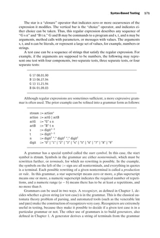
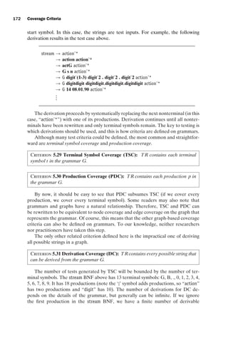
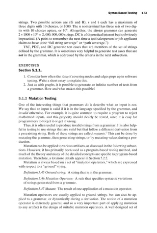
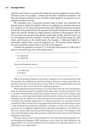
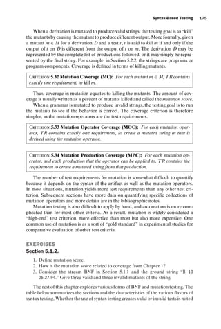
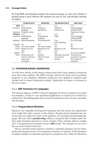
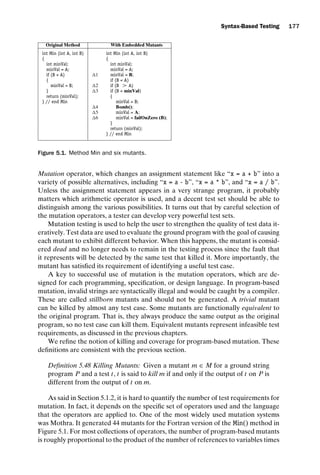
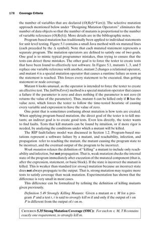
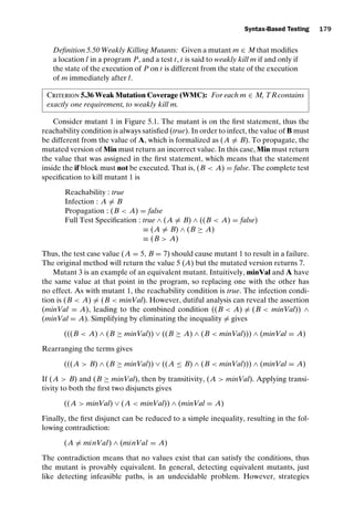
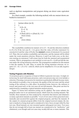
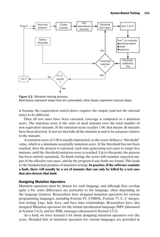
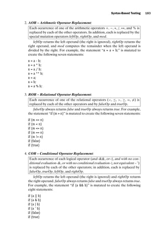
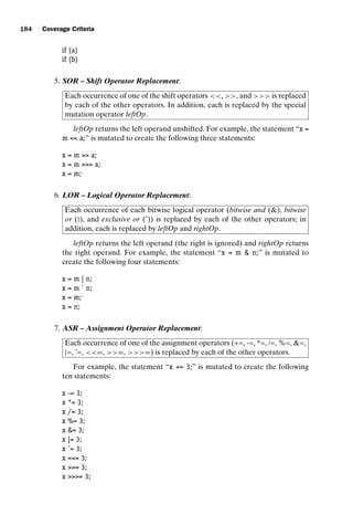
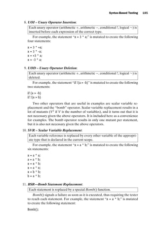
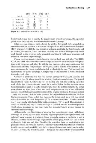
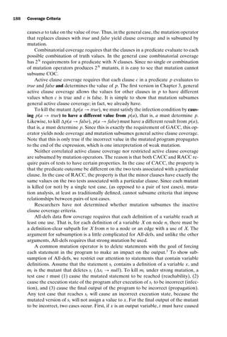
![introtest CUUS047-Ammann ISBN 9780521880381 November 8, 2007 17:13 Char Count= 0
Syntax-Based Testing 189
an execution of a subpath from the deleted definition of x to the output without an
intervening definition (def-clear). Since the output is considered a use, this satisfies
the criterion. Second, if x is not an output variable, then not defining x at si must
result in an incorrect output state. This is possible only if x is used at some later
point during execution without being redefined. Thus, t satisfies the all-defs crite-
rion for the definition of x at si , and the mutation operator yields all-defs, ensuring
that mutation subsumes all-defs.
It is possible to design a mutation operator specifically to subsume all-uses, but
such an operator has never been published or used in any tool.
EXERCISES
Section 5.2.
1. Provide reachability conditions, infection conditions, propagation conditions,
and test case values to kill mutants 2, 4, 5, and 6 in Figure 5.1.
2. Answer questions (a) through (d) for the mutant in the two methods, findVal()
and sum().
(a) If possible, find a test input that does not reach the mutant.
(b) If possible, find a test input that satisfies reachability but not infection for
the mutant.
(c) If possible, find a test input that satisfies infection, but not propagation
for the mutant.
(d) If possible, find a test input that kills mutant m.
//Effects: If numbers null throw NullPointerException //Effects: If x null throw NullPointerException
// else return LAST occurrence of val in numbers[] // else return the sum of the values in x
// If val not in numbers[] return -1
1. public static int findVal(int numbers[], int val) 1. public static int sum(int[] x)
2. { 2. {
3. int findVal = -1; 3. int s = 0;
4. 4. for (int i=0; i x.length; i++) }
5. for (int i=0; inumbers.length; i++) 5. {
5’.// for (int i=(0+1); inumbers.length; i++) 6. s = s + x[i];
6. if (numbers [i] == val) 6’. // s = s - x[i]; //AOR
7. findVal = i; 7. }
8. return (findVal); 8. return s;
9. } 9. }
3. Refer to the TestPat program in Chapter 2. Consider Mutant A and Mutant B
given below:
(a) If possible, find a test case that does not reach the mutant.
(b) If possible, find a test input that satisfies reachability but not infection for
the mutant.
(c) If possible, find a test input that satisfies infection, but not propagation
for the mutant.
(d) If possible, find a test input that kills mutant m.
(a) while (isPat == false isub + patternLen - 1 subjectLen)
while (isPat == false isub + patternLen - 0 subjectLen) // Mutant A
(b) isPat = false;
isPat = true; // Mutant B
4. Why does it make sense to remove ineffective test cases?](https://image.slidesharecdn.com/introductiontosoftwaretesting-221201191322-f16668ac/85/Introduction-to-Software-Testing-pdf-213-320.jpg)
![introtest CUUS047-Ammann ISBN 9780521880381 November 8, 2007 17:13 Char Count= 0
190 Coverage Criteria
5. Define 12 mutants for the following method cal() using the effective mutation
operators given previously. Try to use each mutation operator at least once.
Approximately how many mutants do you think there would be if all mutants
for cal were created?
public static int cal (int month1, int day1, int month2, int day2, int year)
{
//***********************************************************
// Calculate the number of Days between the two given days in
// the same year.
// preconditions : day1 and day2 must be in same year
// 1 = month1, month2 = 12
// 1 = day1, day2 = 31
// month1 = month2
// The range for year: 1 ... 10000
//***********************************************************
int numDays;
if (month2 == month1) // in the same month
numDays = day2 - day1;
else
{
// Skip month 0.
int daysIn[] = {0, 31, 0, 31, 30, 31, 30, 31, 31, 30, 31, 30, 31};
// Are we in a leap year?
int m4 = year % 4;
int m100 = year % 100;
int m400 = year % 400;
if ((m4 != 0) || ((m100 ==0) (m400 != 0)))
daysIn[2] = 28;
else
daysIn[2] = 29;
// start with days in the two months
numDays = day2 + (daysIn[month1] - day1);
// add the days in the intervening months
for (int i = month1 + 1; i = month2-1; i++)
numDays = daysIn[i] + numDays;
}
return (numDays);
}
6. Define 12 mutants for the following method power() using the effective mu-
tation operators given previously. Try to use each mutation operator at least
once. Approximately how many mutants do you think there would be if all
mutants for power() were created?](https://image.slidesharecdn.com/introductiontosoftwaretesting-221201191322-f16668ac/85/Introduction-to-Software-Testing-pdf-214-320.jpg)
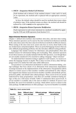
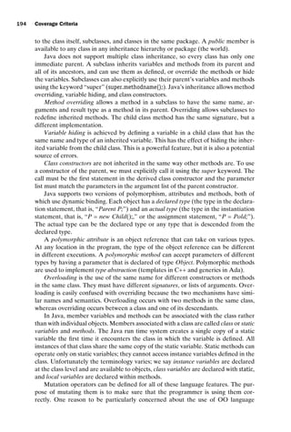

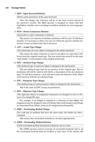
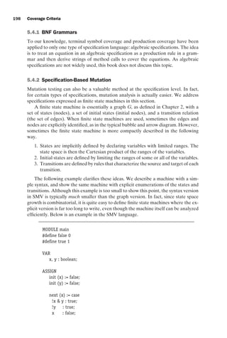
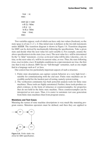
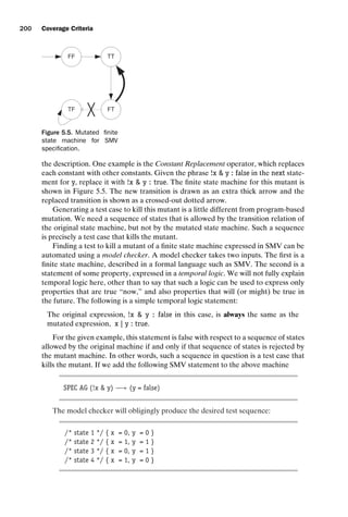
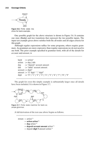
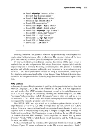
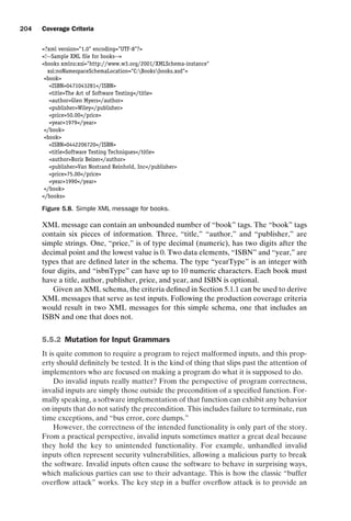
![introtest CUUS047-Ammann ISBN 9780521880381 November 8, 2007 17:13 Char Count= 0
Syntax-Based Testing 205
?xml version=1.0 encoding=UTF-8?
xs:schema xmlns:xs=http://www.w3.org/2001/XMLSchema
elementFormDefault=qualified
attributeFormDefault=unqualified
xs:element name=books
xs:annotation
xs:documentationXML Schema for Books/xs:documentation
/xs:annotation
xs:complexType
xs:sequence
xs:element name=book maxOccurs=unbounded
xs:complexType
xs:sequence
xs:element name=ISBN type=xs:isbnType minOccurs=0/
xs:element name=title type=xs:string/
xs:element name=author type=xs:string/
xs:element name=publisher type=xs:string/
xs:element name=price type=xs:decimal fractionDigits=2 minInclusive=0/
xs:element name=year type=yearType/
/xs:sequence
/xs:complexType
/xs:element
/xs:sequence
/xs:complexType
/xs:element
xs:simpleType name=yearType
xs:restriction base=xs:int
xs:totalDigits value=4/
/xs:restriction
/xs:simpleType
xs:simpleType name=isbnType
xs:restriction base=xs:string
xs:pattern value=[0-9]{10}/
/xs:restriction
/xs:simpleType
/xs:schema
Figure 5.9. XML schema for books.
input that is too long to fit into the available buffer. Similarly, a key step in certain
web browser attacks is to provide a string input that contains malicious HTML,
Javascript, or SQL. Software should behave “reasonably” with invalid inputs.
“Reasonable” behavior may not always be defined, but the test engineer is obliged
to consider it anyway.
To support security as well as to evaluate the software’s behavior, it is useful to
produce test cases that contain invalid inputs. A common way to do this is to mu-
tate a grammar. When mutating grammars, the mutants are the tests and we create
valid and invalid strings. No ground string is used, so the notion of killing mutants
does not apply to mutating grammars. Several mutation operators for grammars are
defined below.
1. Nonterminal Replacement:
Every nonterminal symbol in a production is replaced by other nonterminal
symbols.](https://image.slidesharecdn.com/introductiontosoftwaretesting-221201191322-f16668ac/85/Introduction-to-Software-Testing-pdf-229-320.jpg)
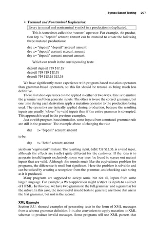
![introtest CUUS047-Ammann ISBN 9780521880381 November 8, 2007 17:13 Char Count= 0
208 Coverage Criteria
validate the messages against the grammar. If they do, it is likely that the software
will usually behave correctly on invalid messages, but testers still need to verify this.
If a validating parser is not used, this can be a rich source for programming mis-
takes. It is also fairly common for programs to use XML messages without having
an explicit schema definition. In this case, it is very helpful for the test engineer to
develop the schema as a first step to developing tests.
XML schemas have a rich collection of built-in datatypes, which come with a
large number of constraining facets. In XML, constraining facets are used to restrict
further the range of values. The example in Figure 5.9 uses several constraining
facets, including fractionDigits, minInclusive, and minOccurs. This suggests further
mutation operators for XML schemas that modify the values of facets. This can
often result in a rich collection of tests for software that use inputs described with
XML.
Given the following four lines in the books schema in Figure 5.9:
xs:element name=ISBN type=xs:isbnType minOccurs=0/
xs:element name=price type=xs:decimal fractionDigits=2 minInclusive=0/
xs:totalDigits value=4/
xs:pattern value=[0-9]{10}/
we might construct the mutants:
xs:element name=ISBN type=xs:isbnType minOccurs=1/
xs:element name=price type=xs:decimal fractionDigits=1 minInclusive=0/
xs:element name=price type=xs:decimal fractionDigits=3 minInclusive=0/
xs:element name=price type=xs:decimal fractionDigits=2 minInclusive=1/
xs:element name=price type=xs:decimal fractionDigits=2 maxInclusive=0/
xs:totalDigits value=5/
xs:totalDigits value=0/
xs:pattern value=[0-8]{10}/
xs:pattern value=[1-9]{10}/
xs:pattern value=[0-9]{9}/
EXERCISES
Section 5.5.
1. Generate tests to satisfy TSC for the bank example grammar based on the
BNF in Section 5.1.1. Try not to satisfy PDC.
2. Generate tests to satisfy PDC for the bank example grammar.
3. Consider the following BNF with start symbol A:
A ::= B@C.B
B ::= BL | L
C ::= B | B.B
L ::= a | b | c | ... | y | z](https://image.slidesharecdn.com/introductiontosoftwaretesting-221201191322-f16668ac/85/Introduction-to-Software-Testing-pdf-232-320.jpg)

![introtest CUUS047-Ammann ISBN 9780521880381 November 8, 2007 17:13 Char Count= 0
210 Coverage Criteria
zero ::= 0
special ::= 1 | 2
other ::= 3 | 4 | 5 | 6 | 7 | 8 | 9
dash ::= -
(a) Classify the following as either phoneNumbers (or not). For non-phone
numbers, indicate the problem.
123-4567
012-3456
109-1212
346-9900
113-1111
(b) Consider the following mutation of the grammar:
exchangePart ::= special ordinary other
If possible, identify a string that appears in the mutated grammar but not
in the original grammar, another string that is in the original but not the
mutated, and a third string that is in both.
7. Java provides a package, java.util.regex, to manipulate regular expressions.
Write a regular expression for URLs and then evaluate a set of URLs against
your regular expression. This assignment involves programming, since input
structure testing without automation is pointless.
(a) Write (or find) a regular expression for a URL. Your regular expression
does not need to be so general that it accounts for every possible URL,
but give your best effort (for example * will not be considered a good
effort). You are strongly encouraged to do some web surfing to find some
candidate regular expressions. One suggestion is to visit the Regular Ex-
pression Library.
(b) Collect a set of URLs from a small web site (such as a set of course web
pages). Your set needs to contain at least 20 (different) URLs. Use the
java.util.regex package to validate each URL against your regular expres-
sion.
(c) Construct a valid URL that is not valid with respect to your regular ex-
pression (and show this with the appropriate java.util.regex call). If you
have done an outstanding job in part 1, explain why your regular expres-
sion does not have any such URLs.
8. Why is the equivalent mutant problem solvable for BNF grammars but not
for program-based mutation? (Hint: The answer to this question is based on
some fairly subtle theory.)
5.6 BIBLIOGRAPHIC NOTES
We trace the use of grammars for testing compilers back to Hanford [150], who mo-
tivated subsequent related work [26, 107, 176, 285, 294]. Maurer’s Data Generation
Language (DGL) tool [231] showed the applicability of grammar-based generation
to many types of software, a theme echoed in detail by Beizer [29].
Legend has it that the first ideas of mutation analysis were postulated in 1971 in
a class term paper by Richard Lipton. The first research papers were published by](https://image.slidesharecdn.com/introductiontosoftwaretesting-221201191322-f16668ac/85/Introduction-to-Software-Testing-pdf-234-320.jpg)
![introtest CUUS047-Ammann ISBN 9780521880381 November 8, 2007 17:13 Char Count= 0
Syntax-Based Testing 211
Budd and Sayward [52], Hamlet [148], and DeMillo, Lipton, and Sayward [99] in the
late 1970s; DeMillo, Lipton, and Sayward’s paper [99] is generally cited as the sem-
inal reference. Mutation has primarily been applied to software by creating mutant
versions of the source, but has also been applied to formal software specifications.
The original analysis of the number of mutants was by Budd [53], who analyzed
the number of mutants generated for a program and found it to be roughly pro-
portional to the product of the number of variable references times the number of
data objects (O(Refs*Vars)). A later analysis [5] claimed that the number of mu-
tants is O(Lines*Refs)–assuming that the number of data objects in a program is
proportional to the number of lines. This was reduced to O(Lines*Lines) for most
programs; this figure appears in most of the literature.
A statistical regression analysis of actual programs by Offutt et al. [269]
showed that the number of lines did not contribute to the number of mutants,
but that Budd’s figure is accurate. The selective mutation approach mentioned
under “Designing Mutation Operators” eliminates the number of data objects so
that the number of mutants is proportional to the number of variable references
(O(Refs)).
A variant of mutation that has been widely discussed is weak mutation [134, 167,
358, 271]. However, experimentation has shown that the difference is very small
[163, 226, 271]. Mutation operators have been designed for various programming
languages, including Fortran IV [19, 56], COBOL [151], Fortran 77 [101, 187], C
[95], C integration testing [94], Lisp [55], Ada [40, 276], Java [185], and Java class
relationships [219, 220].
Research proof-of-concept tools have been built for Fortran IV and 77, COBOL,
C, Java, and Java class relationships. By far the most widely used tool is Mothra, a
mutation system for Fortran 77 that was built in the mid 1980s at Georgia Tech.
Mothra was built under the leadership of Rich DeMillo, with most of the design
done by DeMillo and Offutt, and most of the implementation by Offutt and King,
with help from Krauser and Spafford. In its heyday in the early 1990s, Mothra was
installed at well over a hundred sites and the research that was done to build Mothra
and that later used Mothra as a laboratory resulted in around half a dozen PhD
dissertations and many dozens of papers. As far as we know, the only commercial
tool that supports mutation is by the company Certess, in the chip design industry.
The coupling effect says that complex faults are coupled to simple faults in such
a way that test data that detects all simple faults will detect most complex faults
[99]. The coupling effect was supported empirically for programs in 1992 [263], and
has shown to hold probabilistically for large classes of programs in 1995 [335]. Budd
[51] discussed the concept of program neighborhoods. The neighborhood concept
was used to present the competent programmer hypothesis [99]. The fundamental
premise of mutation testing, as coined by Geist et al. [133] is: in practice, if the
software contains a fault, there will usually be a set of mutants that can be killed
only by a test case that also detects that fault.
The operation of replacing each statement with a “bomb” was called State-
ment ANalysis (SAN) in Mothra [187]. Mothra’s Relational Operator Replacement
(ROR) operator replaces each occurrence of a relational operator (, , ≤, ≥, =, =)
with each other operator and the expression with true and false. The above subsump-
tion proofs used only the latter operators. Mothra’s Logical Connector Replacement
(LCR) operator replaces each occurrence of one of the logical operators (∧, ∨, ≡, =)](https://image.slidesharecdn.com/introductiontosoftwaretesting-221201191322-f16668ac/85/Introduction-to-Software-Testing-pdf-235-320.jpg)
![introtest CUUS047-Ammann ISBN 9780521880381 November 8, 2007 17:13 Char Count= 0
212 Coverage Criteria
with each other operator and the entire expression with true, false, leftop and
rightop. leftop and rightop are special mutation operators that return the left side
and the right side, respectively, of a relational expression. The mutation operator
that removes each statement in the program is called Statement DeLetion (SDL) in
Mothra [187].
A number of authors [14, 15, 37, 298, 350] have used traces from model checkers
to generate tests, including mutation based tests. The text from Huth and Ryan [173]
provides a easily accessible introduction to model checking and discusses use of the
SMV system.
One of the key technologies being used to transmit data among heterogeneous
software components on the Web is the eXtensible Markup Language (XML)
[1, 43]. Data-based mutation defines generic classes of mutation operators. These
mutation operator classes are intended to work with different grammars. The cur-
rent literature [203] cites operator classes that modify the length of value strings and
determine whether or not a value is in a predefined set of values.
NOTES
1 There is no relationship between this use of mutation and genetic algorithms, except that
both make an analogy to biological mutation. Mutation for testing predated genetic algo-
rithms by a number of years.
2 Of course, since mutant detection is undecidable, a heuristic is the best option possible.
3 This goal is in some sense equivalent to the goal of forcing each clause in each predicate to
make a difference.
4 Jester’s web page is http://jester.sourceforge.net/](https://image.slidesharecdn.com/introductiontosoftwaretesting-221201191322-f16668ac/85/Introduction-to-Software-Testing-pdf-236-320.jpg)
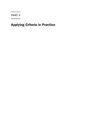

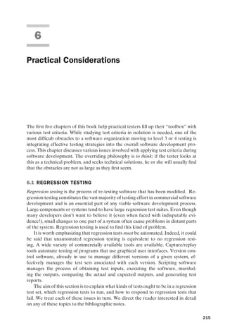
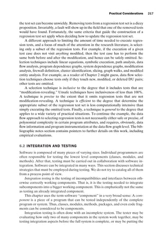
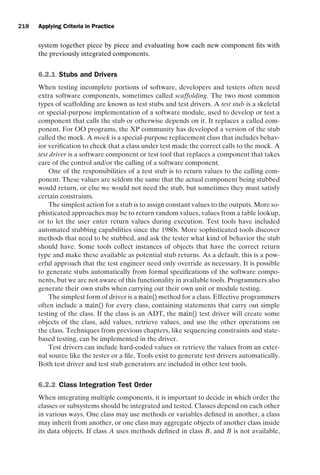
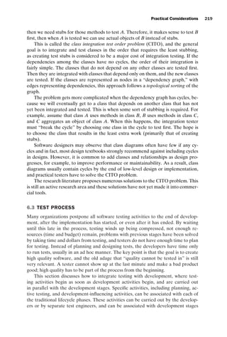
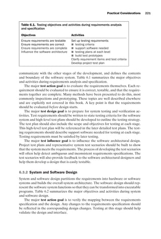
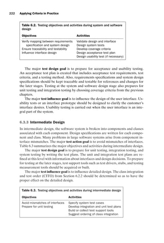
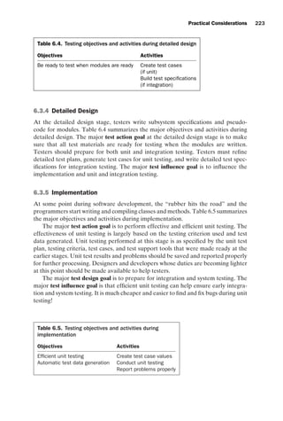


![introtest CUUS047-Ammann ISBN 9780521880381 November 8, 2007 17:13 Char Count= 0
230 Applying Criteria in Practice
knowledge may be needed but not available. Specify contingency plans for
each.
18. Approvals
Specify the names and titles of all persons who must approve this plan, and
include space for them to sign and date the document.
6.5 IDENTIFYING CORRECT OUTPUTS
The main contribution of this book is set of coverage criteria for testing. But no
matter what coverage criterion is used, sooner or later one wants to know whether
a given program executes correctly on a given input. This is the oracle problem in
software testing.
The oracle problem can be surprisingly difficult to solve, and so it helps to have
a range of approaches available. This section describes several common approaches
to the oracle problem.
6.5.1 Direct Verification of Outputs
If you are lucky, your program will come with a specification, and the specification
will be clear as to what output accompanies a given input. For example, a sort pro-
gram should produce a permutation of its input in a specified order.
Having a human evaluate the correctness of a given output is often effective,
but is also expensive. Naturally, it is cheaper to automate this process. Automating
direct verification of the output, when possible, is one of the best methods of check-
ing program behavior. Below is an outline of a checker for sorting. Notice that the
checking algorithm is not another sorting algorithm. It is not only different, it is not
particularly simple. That is, writing output checkers can be hard.
Input: Structure S
Make copy T of S
Sort S
// Verify S is a permutation of T
Check S and T are of the same size
For each object in S
Check if object appears in S and T same number of times
// Verify S is ordered
For each index i but last in S
Check if S[i] = S[i+1]
Unfortunately, direct verification is not always possible. Consider a program that
analyzes Petri nets, which are useful for modeling processes with state. One output
of such analysis is the probability of being in any given state. It is difficult to look at
a given probability and assert that it is correct – after all, it is just a number. How
do you know if all of the digits are, in fact, the right ones? For Petri nets, the final
probabilities cannot easily be related back to the input Petri net.](https://image.slidesharecdn.com/introductiontosoftwaretesting-221201191322-f16668ac/85/Introduction-to-Software-Testing-pdf-254-320.jpg)
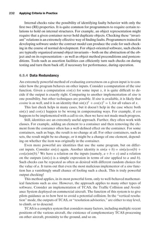
![introtest CUUS047-Ammann ISBN 9780521880381 November 8, 2007 17:13 Char Count= 0
Practical Considerations 233
To apply the technique of data redundancy, suppose we rerun the TCAS soft-
ware with slightly different positions for some or all of the aircraft. We would ex-
pect, in many cases, that the resolution advisory would not change. If the resolution
advisory appeared to be unstable for some closely related inputs, we would have
a strong indication that the pilot might not wish to place much confidence in the
resolution advisory. Back in the laboratory, the TCAS engineers might want to pay
special attention to such inputs – perhaps even regarding them as failures.
The technique illustrated with the TCAS software can be applied to any software
where the input space has some notion of continuity. In any such system, it makes
sense to speak of “nearby” inputs, and in many such systems, the output can be
expected to vary in some piecewise continuous way.
6.6 BIBLIOGRAPHIC NOTES
Binder [33] has an excellent and detailed practical description of regression testing,
in which he claimed that unautomated regression testing is equivalent to no regres-
sion testing. Rothermel and Harrold published the regression testing framework of
inclusiveness, precision, efficiency, and generality [303], and evaluated a safe tech-
nique empirically [153]. Later papers by Li, Harman, and Hierons [208] and Xie and
Notkin [361] are good places to start into the regression testing literature.
The notions of stubs and drivers have been around for decades. They were dis-
cussed in books as far back as the 1970s [88, 104, 165, 249]. Beizer pointed out that
the creation of stubs can be error prone and costly [29]. Current tools such as JUnit
use the term “mock” as a specialized form of a stub [27].
The first paper that defined the CITO problem was by Kung et al. [197]. They
showed that when classes do not have any dependency cycles, deriving an integra-
tion order is equivalent to performing a topological sorting of classes based on
their dependency graph – a well-known graph theory problem. In the presence
of dependency cycles, they proposed a strategy of identifying strongly connected
components (SCCs) and removing associations until no cycles remain. When there
is more than one candidate for cycle breaking, Kung et al.’s approach chooses
randomly.
Most researchers [197, 48, 321, 329] estimated the cost CITO by counting the
number of test stubs that need to be created during integration testing. This method
assumes that all stubs are equally difficult to write. Briand et al. pointed out that
the cost of stubs is not constant and developed a genetic algorithm to solve the
CITO problem [44]. Malloy et al. first tried to consider test stub complexity when
estimating the testing effort [223].
Briand et al. showed that the complexity of stub construction for parent classes
is induced by the likely construction of stubs for most of the inherited member func-
tions [47]. Abdurazik and Offutt developed a new algorithm, based on coupling
analysis, that uses more information about how the stubbed class couples with other
classes to find a cheaper ordering [3].
Some good sources for details about test process and accepted definitions of
terms are IEEE standards [175], BCS standards [317], books by Hetzel [160], De-
Millo et al. [100], Kaner, Falk, and Nguyen [182], Dustin, Rashka, and Paul [109],
and Copeland [90].](https://image.slidesharecdn.com/introductiontosoftwaretesting-221201191322-f16668ac/85/Introduction-to-Software-Testing-pdf-257-320.jpg)
![introtest CUUS047-Ammann ISBN 9780521880381 November 8, 2007 17:13 Char Count= 0
234 Applying Criteria in Practice
Weyuker [341] wrote an early essay identifying the oracle problem and various
approaches to addressing it. Both Meyer [241] and Liskov [355] talk about how to
articulate checkable assertions in the context of the contract model. Several com-
mercial tools support assertion checking.
The notion of building multiple versions was championed in the fault-tolerance
context by a number of authors, most vocally by Avizienis [22]. Limits on reliability
for multiversion software were first explored experimentally by Knight and Leveson
[188], then theoretically by Eckhardt and Lee [110] and Littlewood and Miller [214],
and in a different context by Geist et al. [133]. Multiversion software actually works
better for testing than for fault tolerance. If two versions of the program behave
differently on the same inputs, then we know we have found a good test, and at least
one of the versions is wrong. In particular, it is helpful to view regression testing as
a multiversion testing arrangement.
Blum and Kannan [38] and Lipton [210] give theoretical treatments of data re-
dundancy for certain mathematically well-defined problems; Ammann and Knight
[18] provide a less powerful, but more widely applicable, approach.
NOTES
1 If S is underdetermined, then the requirement S(t) = P(t) is not correct. Instead, S should
be viewed as allowing a set of possible outputs, and the correctness constraint is that P
produces one of them, namely P(t) ∈ S(t).
2 If we wish, we can rewrite the cos(x) calls to sin(π/2 − x) calls, but this is not strictly nec-
essary.](https://image.slidesharecdn.com/introductiontosoftwaretesting-221201191322-f16668ac/85/Introduction-to-Software-Testing-pdf-258-320.jpg)
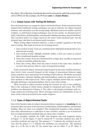
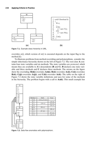
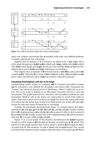
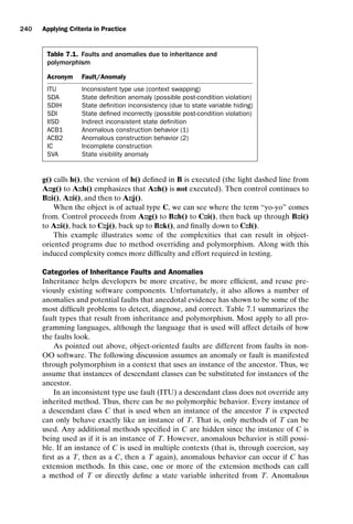
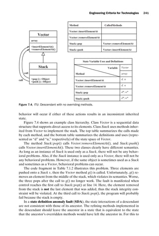
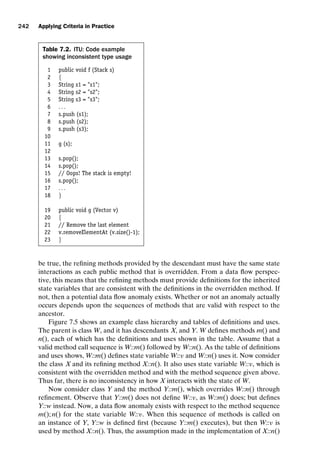
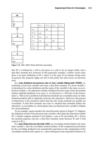
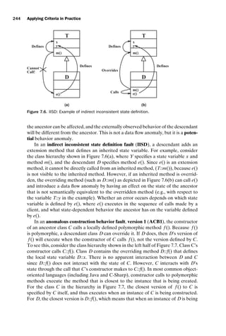
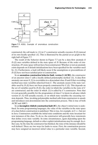
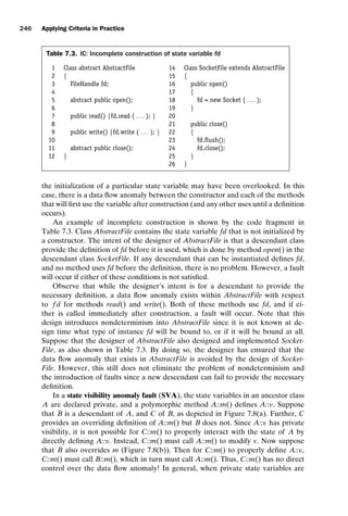
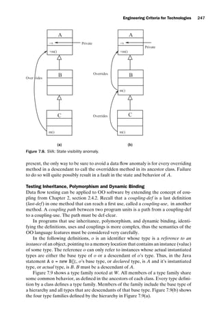
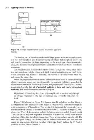
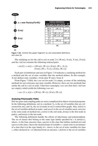
![introtest CUUS047-Ammann ISBN 9780521880381 November 8, 2007 17:13 Char Count= 0
250 Applying Criteria in Practice
f()
m()
n()
object-oriented
direct coupling
data flow
use
def
m ()
n ()
F()
m()
n()
object-oriented
indirect coupling
data flow
m ()
n ()
A()
B()
use
def
A ()
B ()
m() and n() could be in the same class or accessing a
global or other non-local variable.
Figure 7.11. Def-use pairs in object-oriented software.
that are indirectly defined within m() and i-uses(m) is the set of variables used by
m().
A coupling sequence is a pair of nodes that call two methods in sequence; the first
method defines a variable and the second uses it. Both calls must be made through
the same instance object. The calling method is called the coupling method f(), and
it calls m(), the antecedent method, to define x, and n(), the consequent method, to
use x. This is illustrated in Figure 7.11 (repeated from Chapter 2). If the antecedent
or consequent method is the same as the coupling method, that is a special case that
is handled implicitly. If the antecedent or consequent method is called from another
method that is called by f(), this an indirect data flow (right side of Figure 7.11),
which we do not discuss.
The control flow schematic shown in Figure 7.12 illustrates the coupling method
calling both the antecedent and consequent methods. The schematic abstracts away
the details of the control flow graph and shows only nodes that are relevant to cou-
pling analysis. The thin line segments represent control flow and the thicker lines
indicate control flow that is part of a coupling path. The line segments can represent
multiple sub-paths. A path may be annotated with a transmission set such as [o, o.v],
which contains variables for which the path is definition-clear.
Assuming that the intervening sub-paths are def-clear with respect to the state
variable o.v, the path in Figure 7.12 from h to i to j to k and finally l forms a trans-
mission path with respect to o.v. The object o is called the context variable.
Every coupling sequence sj,k has some state variables that are defined by the
antecedent method and then used by the consequent method. This set of variables
is the coupling set t
sj,k
of sj,k and is defined as the intersection of those variables
defined by m() (an indirect-def or i-def) and used by n() (an indirect use or i-use)
through the instance context provided by a context variable o that is bound to an
instance of t. Which versions of m() and n() execute is determined by the actual type
t of the instance bound to o. The members of the coupling set are called coupling
variables.
Coupling sequences require that there be at least one def-clear path between
each node in the sequence. Identifying these paths as parts of complete sequences of
nodes results in the set of coupling paths. A coupling path is considered to transmit
a def of a variable to a use.](https://image.slidesharecdn.com/introductiontosoftwaretesting-221201191322-f16668ac/85/Introduction-to-Software-Testing-pdf-274-320.jpg)
![introtest CUUS047-Ammann ISBN 9780521880381 November 8, 2007 17:13 Char Count= 0
Engineering Criteria for Technologies 251
Coupling
Method
i o.m()
k o.n()
j def(o.v)
h def(o)
m()
f()
n()
l use(o.v)
Coupling
Sequence
sj,k
with
respect
to o.v
transmission
path
[o,o.v]
[o]
i-def path
[o.v]
i-use path
[o.v ]
Antecedent
Node
Consequent
Node
Coupling Context
Call site
Call return
Method entry
Statement
Control Flow
Coupling Path
Method exit
Transmission set
[...]
Antecedent
Method
Consequent
Method
Figure 7.12. Control flow schematic for prototypical
coupling sequence.
Each path consists of up to three sub-paths. The indirect-def sub-path is the por-
tion of the coupling path that occurs in the antecedent method m(), extending from
the last (indirect) definition of a coupling variable to the exit node of m(). The
indirect-use sub-path is the portion of the consequent method n() that extends from
the entry node of n() to the first (indirect) use of a coupling variable. The transmis-
sion sub-path is the portion of the coupling path in the coupling method that extends
from the antecedent node to the consequent node, with the requirement that neither
the value of the coupling variable nor the context variable is modified.
Each coupling sequence has a single set of coupling paths for each type of cou-
pling sub-path. These sets are used to form coupling paths by matching together
elements of each set. The set of coupling paths is formed by combining elements
of the indirect-def sub-path set with an element from the transmission sub-path set,
and then adding an element of the indirect-use sub-path set. The complete set of
coupling paths is formed by taking the cross product of these sets.
To see the effects of inheritance and polymorphism on paths, consider the
class diagram shown in Figure 7.13(a). The type family contains the classes A, B,
and C. Class A defines methods m() and n() and state variables u and v. Class
B defines method l() and overrides A’s version of n(). Likewise, C overrides A’s
version of m(). Definitions and uses for each of these methods are shown in
Figure 7.13(b).
Figure 7.14 shows coupling paths for a method that uses the hierarchy in
Figure 7.13(a). Figure 7.14(a) shows the declared type of the coupling variable o is
A, and Figure 7.14(b) shows the antecedent and consequent methods when the ac-
tual type is also A. The coupling sequence sj,k extends from the node j where the
antecedent method m() is called to the call site of the consequent method at node
k. As shown, the corresponding coupling set for sj,k when o is bound to an instance](https://image.slidesharecdn.com/introductiontosoftwaretesting-221201191322-f16668ac/85/Introduction-to-Software-Testing-pdf-275-320.jpg)
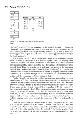
![introtest CUUS047-Ammann ISBN 9780521880381 November 8, 2007 17:13 Char Count= 0
Engineering Criteria for Technologies 253
bind(o, A)
o.m()
o.n()
def(A.v) def(A.u)
[A.v] [A.u]
[o]
[o, A.u]
use(A.v)
[A.v
j
i
k
sj,k
A.m,A.n
= {A.v}
Coupling Method
f()
A.m()
A.n()
transmission
paths
Antecedent Method
Consequent Method
Antecedent
Node
Consequent
Node
Declared
type ofo is A
Coupling Variable
e f
g
A.mb
A.ma
fc
A.nd
def(A.u)
[A.u]
use(A.u)
[A.u]
C.m,B.n
= {A.u}
e
g
C.ma
B.nd
(a) (b)
def(A.v) def(A.u)
[A.v] [A.u]
use(A.u)
[A.u]
A.m,B.n
= {A.u}
A.m()
B.n()
Antecedent Method
Consequent Method
e f
g
A.mb
A.ma
B.nd
C.m()
Antecedent Method
B.n()
Consequent Method
Actual type of
o isB
Actual type of
o is C
Actual type of
o is A
(d)
(c)
O O O
Figure 7.14. Coupling sequence: o of type A (a) bound to instance of A (b), B (c) or C (d).
To account for the possibility of polymorphic behavior at a call site, the def-
inition of a coupling sequence must be amended to handle all methods that can
execute. A binding triple for a coupling sequence contains the antecedent method
m(), the consequent method n(), and the set of coupling variables that result from
the binding of the context variable to an instance of a particular type. The triple
matches a pair of methods p() and q() that can potentially execute as the result of
executing the antecedent and consequent nodes j and k. Each may be from different
classes that are members of the type family defined by c, provided that p() is an over-
riding method for m() or q() is an overriding method for n(). There will be exactly
one binding triple for each class d ∈ family(c) that defines an overriding method for
either m() or n().](https://image.slidesharecdn.com/introductiontosoftwaretesting-221201191322-f16668ac/85/Introduction-to-Software-Testing-pdf-277-320.jpg)
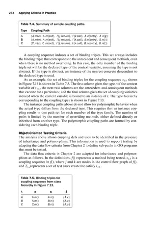
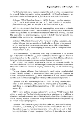
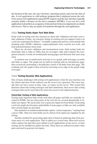
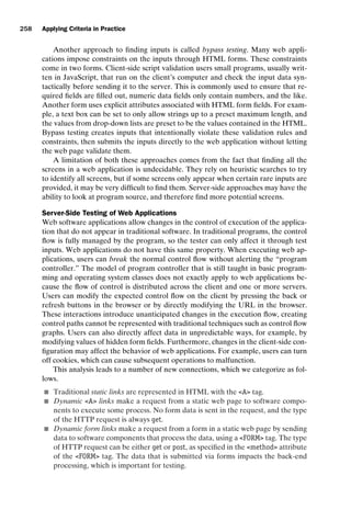
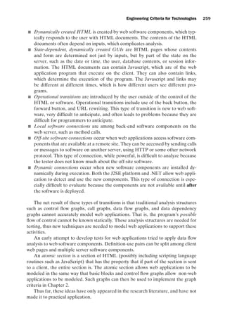
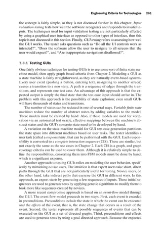
![introtest CUUS047-Ammann ISBN 9780521880381 November 8, 2007 17:13 Char Count= 0
Engineering Criteria for Technologies 265
the number of such pairs grows quickly with the size and constraints on the
software.
Timed automata have also been used to verify sequences of timed action tran-
sitions. This approach uses a reachability analysis to determine what transitions to
test; that is, a graph-based approach. This can suffer from state space explosion for
large dynamic models. One way to ameliorate that problem is to use a sampling
algorithm based on grid-automata and nondeterministic finite-state machines to re-
duce the test effort.
A non-formal model approach uses genetic algorithms. Data are gathered during
execution of the real system and visualized for post analysis. Fitness of a test case is
calculated based on its uniqueness and what exceptions are generated by the systems
and test harness during test execution.
One approach to generating tests is to statically derive execution orders of a
real-time system before it is put into operation. Each execution order is treated as
a separate sequential program, and conventional test methods can be applied. This
only works if all task activation times are fixed.
Most of the above approaches are based on graph criteria (Chapter 2) in one way
or another. A different approach is based on mutation (Chapter 5). In mutation-
based timeliness testing, potential faults are modeled as mutation operators. Mu-
tants that have the potential to violate timeliness are identified, and test cases are
constructed that try to kill the mutants.
Eight types of mutants have been defined. The task set mutation operator
changes the points in time when a resource is taken. The execution time mutation
operator increases or decreases the execution time of a task by a constant time delta.
The hold time shift mutation operator changes the interval of time a resource is
locked. The lock time mutation operator increases or decreases the time when a re-
source is locked. The unlock time mutation operator change when a resource is un-
locked. The precedence constraint mutation operator adds or removes precedence
constraint relations between pairs of tasks. The inter-arrival time mutant operator
decreases the inter-arrival time between requests for a task execution by a constant
time . The pattern offset mutation operator changes the offset between two such
patterns by a constant time units. Test cases to kill timeliness mutants are created
by model-checking and by genetic algorithms.
7.5 BIBLIOGRAPHIC NOTES
The bibliographic notes in this chapter follow the order of the sections above,
object-oriented software, web applications, GUIS, and real-time and embedded
software.
Good sources for building abstractions in object-oriented language are by Meyer
[241], Liskov, Wing and Guttag [212, 213], and Firesmith [119]. Liskov, Wing
and Guttag contributed the substitution principle. Discussions about whether the
substitution principle should always be followed can be found by Lalonde and Pugh
[199] and Taivalsaari [323].
Binder pointed out how OO relationships tend to be complex [35]. and Berard
first articulated the differences in integration [31]. The connection between inheri-
tance, polymorphism, dynamic binding and undecidability is due to Barbey [24].](https://image.slidesharecdn.com/introductiontosoftwaretesting-221201191322-f16668ac/85/Introduction-to-Software-Testing-pdf-289-320.jpg)
![introtest CUUS047-Ammann ISBN 9780521880381 November 8, 2007 17:13 Char Count= 0
266 Applying Criteria in Practice
Doong and Frankl [105] wrote a seminal paper on state-based object-oriented
testing. The three class testing levels of intra-method testing, inter-method testing,
and intra-class testing are due to Harrold and Rothermel [152]; Gallagher and Offutt
[132] added inter-class testing.
Several papers focused on inter-method and intra-class testing [118, 152, 281,
315], testing interactions between classes and their users [284] and system-level test-
ing [181].
The yo-yo graph was provided by Alexander and Offutt [266], and based on
the discussion from Binder that execution can sometimes “bounce” up and down
among levels of inheritance [35]. The categories of OO faults and anomalies are
due to Alexander and Offutt [9, 266]. Most of the OO coupling and data flow test
criteria were developed by Alexander as part of his thesis work [7, 10, 11].
The idea of using a graph to represent static web sites was initially proposed by
Ricca and Tonella [300]. Kung et al. [198, 215] also developed a model to represent
web sites as a graph, and provided preliminary definitions for developing tests based
on the graph in terms of web page traversals. Their model includes static link transi-
tions and focuses on the client side with only limited use of the server software. They
define intra-object testing, where test paths are selected for the variables that have
def-use chains within the object, inter-object testing, where test paths are selected
for variables that have def-use chains across objects, and inter-client testing, where
tests are derived from a reachability graph that is related to the data interactions
among clients.
Benedikt, Freire, and Godefroid [30] initiated the idea of “action sequences” in
a tool called VeriWeb. VeriWeb’s testing is based on graphs where nodes are web
pages and edges are explicit HTML links, and the size of the graphs is controlled by
a pruning process.
Elbaum, Karre, and Rothermel [112, 113] proposed the idea of “user session
data” to generate test cases for web applications.
Liu, Kung, Hsia, and Hsu [216] first tried to apply data flow analysis to web
software components. The focus was on data interactions and their model did not
incorporate dynamically generated web pages or operational transitions.
Bypass testing is due to Offutt, Wu, Du, and Huang [278]. The analysis about the
connections in web applications in Section 7.2.2 is due to Offutt and Wu [359, 360].
They also introduced the concept of an atomic section.
Di Lucca and Di Penta [217] proposed testing sequences through a web applica-
tion that incorporates some operational transitions, specifically focusing on the back
and forward button transitions. Timewise, this paper is the first published work ad-
dressing operational transitions, although it postdates the earlier technical report by
Offutt and Wu [359]. Di Lucca and Di Penta’s model focused on the browser capa-
bilities without considering the server-side software or dynamically generated web
pages.
The use of syntax-based testing techniques to create XML messages as tests for
web services components is due to Offutt and Wu [279, 280].
Nielson [253] provides an excellent overview of the importance of web usability
in general and includes a discussion of usability testing.
Early work in using state-machine models to generate tests for GUIs are by
Clarke [79], Chow [77], Esmiloglu [115], and Bernhard [32]. The variable finite state
machine model is due to Shehady et al. [312].](https://image.slidesharecdn.com/introductiontosoftwaretesting-221201191322-f16668ac/85/Introduction-to-Software-Testing-pdf-290-320.jpg)
![introtest CUUS047-Ammann ISBN 9780521880381 November 8, 2007 17:13 Char Count= 0
Engineering Criteria for Technologies 267
The concept of partitioning the GUI state space into responsibilities is due to
White et al. [346, 347]. The idea of modeling novice user behavior to generate tests is
due to Kasik [183]. The event flow model has been extensively developed by Memon
et al. [235, 236, 237, 238, 239, 240, 250].
The literature on testing real-time and embedded software is much smaller than
some of the other topics in this book. The concepts presented in this chapter only
introduce the topic. The following references are far from complete, but will help
introduce the interested reader to the field.
General knowledge on real-time software systems and timeliness can be found
in Young [364], Ramamrithaam [296], and Schütz [309]. Many of the issues in testing
real-time systems were published by Schütz [310]. This probe-effect is due to Gait
[131]. Timeliness was discussed by Verissimo and Kopetz [331].
The method of using Petri nets is due to Braberman et al. [42]. Cheung et al.
[68] presented a framework for testing multimedia software, including temporal re-
lations between tasks with “fuzzy” deadlines.
The framework for testing time constraints using constraint graphs and process
algebras is due to Clarke and Lee [78].
The clock region graph approach is by Petitjean and Fochal [287]. Krichen
and Tripakis [193] addressed limitations in applicability of previous client-side ap-
proaches and suggested a method for conformance testing using nondeterministic
and partially observable models. Their testing criteria were inspired by Hessel et al.
[159].
The temporal logic approach is due to Mandrioli et al. [225], who based their
work on SanPietro et al. [308]. The timed automata approach is due to Cardell-
Oliver and Glover [61]. Another automata-based approach was by En-Nouaary et
al. [114], who introduced the sampling algorithm using grid-automata. Similarly,
Nielsen and Skou [252] use a subclass of timed automata to specify real-time ap-
plications. Raymond et al. [299] presented a method to generate event sequences
for reactive systems.
The genetic algorithm approach is due to Watkins et al. [337]. Morasca and Pezze
[245] proposed a method for testing concurrent and real-time systems that uses high-
level Petri nets for specification and implementation. The technique of statically
deriving execution orders is due to Thane [326] and Pettersson and Thane [288].
Wegener et al. explored the capabilities of genetic algorithms for testing temporal
properties of real-time tasks [338], attempting to create inputs that produced the
worst and best-case execution times. The application of mutation to timeliness faults
was by Nilsson [254, 255, 257, 256].
NOTES
1 Researchers interpret “interesting” to mean having fun problems to solve, but developers,
especially managers, should interpret “interesting” as a threat to timely completion of a
quality product.
2 The URL is http://www.softwareqatest.com/qatweb1.html](https://image.slidesharecdn.com/introductiontosoftwaretesting-221201191322-f16668ac/85/Introduction-to-Software-Testing-pdf-291-320.jpg)
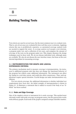
![introtest CUUS047-Ammann ISBN 9780521880381 November 8, 2007 17:13 Char Count= 0
Building Testing Tools 269
Original Function With Instrument
public int min (A, B) public int min (A, B)
{ {
int m = A; int m = A;
if (A B) if (A B)
{ {
m = B; Mark: “if body has been reached”
} m = B;
return (m); }
} return (m);
}
Figure 8.1 Initial example of instrumentation.
An array is created that is indexed by the node numbers (called nodeCover []). Next,
the following instrument is inserted at each node i: “nodeCover [i]++;.”
It is important that the nodeCover[] array be “persistent,” that is, it must be saved
to disk after each test case. This allows results to be accumulated across multiple
test cases. After some tests have been executed, every node i for which nodeCover[i]
is zero has not been covered. If nodeCover[i] is not zero, its value represents the
number of times node i was reached.
This process is shown in Figure 8.2. The nodeCover[] array must be read before
execution starts and is shown on node 1 in the figure. Each node is annotated with
the appropriate instrumentation (“nc” is used as an abbreviation for “nodeCover”).
An automated coverage analysis tool can insert the instruments at the beginning
1
2
4 5
3
6
7
8
10
9
int nodeCover [ ] = {0,0,0,0,0,0,0,0,0,0}
Read (nodeCover [ ]);
nodeCover [1] ++;
nc [3]++;
nc [5]++;
nc [9]++;
nc [6]++;
nc [10]++;
nc [8]++;
nc [7]++;
nc [4]++;
nc [2]++;
Figure 8.2. Node coverage instrumentation.](https://image.slidesharecdn.com/introductiontosoftwaretesting-221201191322-f16668ac/85/Introduction-to-Software-Testing-pdf-293-320.jpg)
![introtest CUUS047-Ammann ISBN 9780521880381 November 8, 2007 17:13 Char Count= 0
270 Applying Criteria in Practice
1
2
4 5
3
6
7
8
10
9
int edgeCover [ ] = {0,0,0,0,0,0,0,0,0,0,0,0,0}
Read (edgeCover [ ]);
ec [2]++;
ec [1]++;
ec [9]++;
ec [10]++;
ec [11]++;
ec [7]++;
ec [12]++; ec [13]++;
ec [8]++;
ec [6]++;
ec [5]++;
ec [4]++;
ec [3]++;
Figure 8.3. Edge coverage instrumentation.
of basic blocks or in front of individual statements. The latter is less accurate, but
simpler to implement, so is fairly common in commercial tools. The instruments can
also be inserted in the source code and then compiled separately, into executable
files, or into intermediate forms such as Java ByteCode. Java Reflection could also
be used to insert instrumentation, although we know of no tool that uses this tech-
nique.
Instrumenting for edge coverage is only slightly more complicated than for node
coverage. Each edge in the graph is assigned a unique identifier number. An array
is created that is indexed by the edge numbers (edgeCover []). Next the following
instrument is inserted onto each edge i: “edgeCover[i]++;.”
This process is illustrated in Figure 8.3. As with node coverage, the edgeCover[]
array must be read before execution starts. Each node in Figure 8.3 is anno-
tated with “ec” as an abbreviation for “edgeCover.” The instrumentation for some
edges is sometimes omitted if coverage is implied by another. For example, in Fig-
ure 8.3, any test that causes edge 3 to be executed will also cause edge 5 to be
executed.
Some structures do not explicitly represent all edges. For example, the follow-
ing program source does not have a location for the instrumentation on the else
edge:
if (isPrime)
{ // save it!
primes[numPrimes] = curPrime;
numPrimes++;
}](https://image.slidesharecdn.com/introductiontosoftwaretesting-221201191322-f16668ac/85/Introduction-to-Software-Testing-pdf-294-320.jpg)
![introtest CUUS047-Ammann ISBN 9780521880381 November 8, 2007 17:13 Char Count= 0
Building Testing Tools 271
Therefore the else clause must be explicitly added to instrument for branch cov-
erage:
if (isPrime)
{ // save it!
primes[numPrimes] = curPrime;
numPrimes++;
}
else
edgeCover[5]++;
8.1.2 Data Flow Coverage
Data flow coverage is somewhat more complicated than node and edge coverage.
The primary difference is that the criterion is based on two locations in the program:
one for the definition and one for the use. As with node coverage, each node is
assigned a unique number, but two arrays are used. Since edges can also contain
uses, each edge must also be assigned a unique number. The technique is to use one
array to keep track of definitions and another to keep track of uses.
At each location where variable x is defined, the statement “defCover[x] = i;” is
added, where i is the node number. This means that defCover[x] will store the last
location where x was defined. The second array keeps track of uses. For a variable
x, useCover[] stores uses on a node or edge. For each node or edge i where a variable
x is used, the statement “useCover[i, x, defCover[x]]++;” is added. The array loca-
tion useCover[i, x, defCover[x]] indicates that x is used at node (or edge) i and the
definition from node defCover[x] has reached the use at i.
Figure 8.4 illustrates instrumentation for All-uses. Variables x and y are defined
(through parameter passing or assignments) at node 1 and y is redefined at node
2. Variable x is used at nodes 4 and 5 and y is used at node 6. If the path 1, 2,
1
2
4 5
3
6
def (x, y)
defCover [x] = 1;
defCover [y] = 1;
def (y)
use (x)
use (x)
use (y)
defCover [y] = 2;
useCover [4, x, defCover [x]] ++;
useCover [5, x, defCover [x]] ++;
useCover [6, y, defCover [y]] ++;
7
10
9
8
11
13
12
Figure 8.4. All uses coverage instrumentation.](https://image.slidesharecdn.com/introductiontosoftwaretesting-221201191322-f16668ac/85/Introduction-to-Software-Testing-pdf-295-320.jpg)
![introtest CUUS047-Ammann ISBN 9780521880381 November 8, 2007 17:13 Char Count= 0
272 Applying Criteria in Practice
6 is toured, then when the statement “useCover[6, y, defCover[y]]++;” at node 6 is
reached, defCover[y] will be 2, and coverage of DU pair [2, 6] will be recorded. If,
however, the path 1, 3, 4, 6 is toured, then defCover[y] will be 1 when node 6 is
reached, so coverage of DU pair [1, 6] will be recorded.
All-uses instrumentation is a little hard to grasp at first. If in doubt, the reader
should walk through a couple of simple examples to verify that the useCover[] array
stores the needed information. After execution, the useCover[] array records zeros
for DU pairs that have not been covered, and nonzero values for DU pairs that
have been. Other analysis, not covered in this book, is required to determine which
definitions can reach which uses, and which DU pairs have def-clear paths. Pairs of
definitions and uses without def-clear paths between them will result in zero values
in the useCover[] array.
8.1.3 Logic Coverage
We show how to instrument for just one of the logic coverage criteria from Chap-
ter 3. The others are similar.
Instrumenting for the logic coverage criteria requires more instrumentation than
structural or data flow instrumentation. The abstract view is whenever a predicate
is reached, each clause in each predicate must be evaluated separately to determine
which of the test requirements on the predicate have been satisfied. These evalua-
tions are implemented in separate methods that mark special arrays to record which
test requirements have been satisfied.
Consider the graph in Figure 8.5(a). The first predicate is (A B) and it results
in the test requirements (F, T), (T, T), and (T, F). Figure 8.5(b) gives the method that
is called by the instrumented statement at node 1. It implements the predicate on
the edge (1, 2) and marks the array CACCCover[] to indicate which test requirement
has been satisfied.
The second predicate, C (D || E), has three clauses and because of the “or”
condition, some choices are possible in the test requirements. This is illustrated in
Figure 8.5(c). Again the predicate is evaluated, one clause at a time, and the ap-
propriate test requirement coverage is recorded. Note that CACCCover[5] is recorded
in three different places. This represents the fact that one test requirement can be
satisfied by one of three clause truth assignments.
A different approach to instrumenting for the ACC criteria is, for each predicate,
simply to record the combination of truth values for each clause in that predicate.
Such an approach is not appropriate if clauses have side effects, or if predicates rely
on short circuit evaluation, such as testing an array index prior to dereferencing the
array. However, the advantage of such an approach is that the analysis of satisfaction
of the ACC criteria is separated from the code under instrumentation. Hence, the
criteria analysis engine can be applied to ACC coverage data collected from any
artifact.
8.2 BUILDING MUTATION TESTING TOOLS
Mutation was described in Chapter 5. It is widely regarded as the most difficult cri-
terion to satisfy, and empirical studies have consistently found it to be stronger than](https://image.slidesharecdn.com/introductiontosoftwaretesting-221201191322-f16668ac/85/Introduction-to-Software-Testing-pdf-296-320.jpg)
![introtest CUUS047-Ammann ISBN 9780521880381 November 8, 2007 17:13 Char Count= 0
Building Testing Tools 273
(a)
CACC_Mark_1 (A, B)
{
if (!A)
{ // Don’t allow short circuit
if (B)
CACCCover[1]++;
}
else // A
{
if (B)
CACCCover [2]++;
else
CACCCover[3]++
}
}
1
2
4 5
3
6
CACC_Mark_1 (A, B)
if (A B)
if (C (D || E))
CACC_Mark_2 (C, D, E)
A B CACCCover [ ]
F t 1
T t 2
t F 3
t T
CACC_Mark_2 (C, D, E)
{
if (! C)
{
if (D || E)
CACCCover [4]++;
}
else if (! D)
{
if (! E)
CACCCover [6]++;
else
{
CACCCover [5]++;
CACCCover [8]++;
}
}
else // C and D
if (! E)
{
CACCCover [5]++;
CACCCover [7]++;
}
else
CACCCover [5]++;
}
C (D || E) CC [ ]
F 4
T 5
t F f 6
t T f 7
t f F
t f T 8
{
t t
t f
f t
}
(b)
(c)
Figure 8.5. Correlated active clause coverage instrumentation.
other criteria in terms of the number of faults it can detect. It is also all but im-
possible to apply by hand; thus automation is a must. Not surprisingly, automating
mutation is more complicated than automating other criteria. Simply adding instru-
mentation to the program does not work. The literature on building mutation testing
systems is large, and we have lots of experience, at least in the research community.
And luckily, changes in language design and advances in tools have made this kind
of system much easier to build. This section explores issues with building mutation
systems and explains how a mutation testing system can be built in a reasonably
efficient manner.
The first thing to realize about a mutation testing system is that it is in large part
a language system. Programs must be parsed, modified and executed. Please refer](https://image.slidesharecdn.com/introductiontosoftwaretesting-221201191322-f16668ac/85/Introduction-to-Software-Testing-pdf-297-320.jpg)
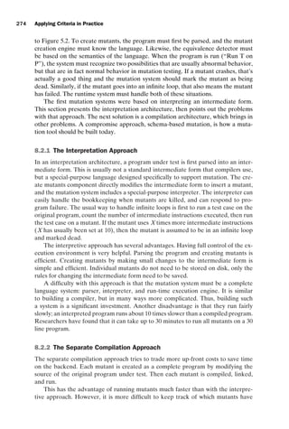
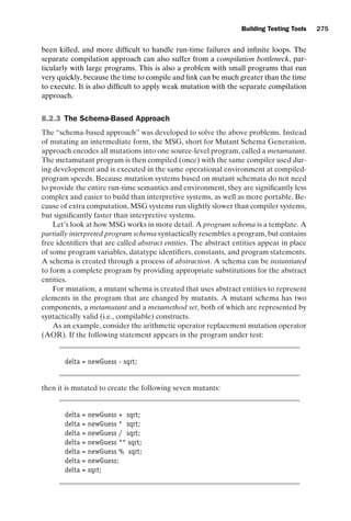
![introtest CUUS047-Ammann ISBN 9780521880381 November 8, 2007 17:13 Char Count= 0
Building Testing Tools 277
which is the ability to introspect data structures, but does not directly support modi-
fication of the program behavior. Several reflection systems have been built and are
available to support compile-time and load-time reflection. As of this writing, the
technology for run-time reflection is still developing.
Bytecode translation is similar to reflection, but uses a different approach. Byte-
code translation inspects and modifies the intermediate representation of Java pro-
grams, bytecode. Since it directly handles bytecode, it has some advantages over
separate compilation and MSG approaches. First, it can process an off-the-shelf
program or library that is supplied without source code. Second, it can run at
load time, when the Java Virtual Machine loads a class file. Bytecode transla-
tion is not as efficient as run-time reflection, but presently the technology is more
stable.
8.2.5 Implementing a Modern Mutation System
A modern mutation system would use a combination of MSG for mutants that do
not affect the structure of the program, and reflection for mutants that do. Although
still more complicated than instrumenting for statement or branch coverage, the
amount of programming is significantly less than for interpretive systems. This is
the approach taken by the muJava system mentioned in Chapter 5.
8.3 BIBLIOGRAPHIC NOTES
We were not able to find any published references for how to do instrumentation.
However, researchers and tool builders have been using techniques such as what we
have presented for many years.
PIMS [5, 52, 54, 211], an early mutation testing tool, pioneered the general pro-
cess typically used in mutation testing of creating mutants (of Fortran IV programs),
accepting test cases from the users, and then executing the test cases on the mutants
to decide how many mutants were killed.
In 1987, this same process (of add test cases, run mutants, check results, and
repeat) was adopted and extended in the Mothra mutation toolset [96, 101, 262, 268],
which provided an integrated set of tools, each of which performed an individual,
separate task to support mutation analysis and testing. Although other mutation
testing tools have been developed since Mothra [95, 97, 220, 330], Mothra is likely
the most widely known mutation testing system extant.
Many of the advances in mutation testing addressed the performance cost. They
usually follow one of three strategies: do fewer, do smarter, or do faster.
The do fewer approaches try to run fewer mutant programs without incurring
unacceptable information loss. Mutant sampling [4, 53, 356] uses a random sample
of the mutants and is the simplest do fewer approach. A 10% sample of mutant
programs, for example, was found to be only 16% less effective than a full set in
ascertaining fault detection effectiveness. The effects of varying the sampling per-
centage from 10% to 40% in steps of 5% were later investigated by Wong [356].
An alternative sampling approach is proposed by S
. ahinoğlu and Spafford [106] that
does not use samples of some a priori fixed size, but rather, based on a Bayesian
sequential probability ratio test, selects mutant programs until sufficient evidence](https://image.slidesharecdn.com/introductiontosoftwaretesting-221201191322-f16668ac/85/Introduction-to-Software-Testing-pdf-301-320.jpg)
![introtest CUUS047-Ammann ISBN 9780521880381 November 8, 2007 17:13 Char Count= 0
278 Applying Criteria in Practice
has been collected to determine that a statistically appropriate sample size has been
reached.
Wong and Mathur suggested the idea of selective mutation as applying mutation
only to the most critical mutation operators being used [230, 357]. This idea was
later developed by Offutt et al. [269] who identified a set of selective operators for
Fortran-77 with Mothra. Results showed that selective mutation provide almost the
same test coverage as nonselective mutation. The operators presented in this Chap-
ter are based on the selective approach.
The use of nonstandard computer architecture has been explored as a do smarter
approach. This approach distributes the computational expense over several ma-
chines. Work has been done to adapt mutation analysis system to vector processors
[229], SIMD machines [192], Hypercube (MIMD) machines [75, 275], and Network
(MIMD) computers [365]. Because each mutant program is independent of all other
mutant programs, communication costs are fairly low. At least one tool was able to
achieve almost linear speedup for moderate sized program functions [275].
Weak mutation [167] is another do smarter approach. It is an approximation tech-
nique that compares the internal states of the mutant and original program imme-
diately after execution of the mutated portion of the program. Experimentation has
shown that weak mutation can generate tests that are almost as effective as tests
generated with strong mutation, and that at least 50% and usually more of the ex-
ecution time is saved. The Leonardo system [270, 271], which was implemented as
part of Mothra, did two things. It implemented a working weak mutation system
that could be compared easily with strong mutation, and evaluated the extent/firm
concept by allowing comparisons to be made at four different locations after the
mutated component: (1) after the first evaluation of the innermost expression sur-
rounding the mutated symbol, (2) after the first execution of the mutated statement,
(3) after the first execution of the basic block that contains the mutated statement,
and (4) after each execution of the basic block that contains the mutated statement
(execution stops as soon as an invalid state is detected).
In another “do smarter” approach, Fleyshgakker and Weiss describe algorithms
that improve the run-time complexity of conventional mutation analysis systems
at the expense of increased space complexity [120]. By intelligently storing state
information, their techniques factor the expense of running a mutant over several
related mutant executions and thereby lower the total computational costs.
In the separate compilation approach, each mutant is individually created, com-
piled, linked, and run. The Proteum system [95] is an example of the separate compi-
lation approach. When mutant run times greatly exceed individual compilation/link
times, a system based on such a strategy will execute 15–20 times faster than an in-
terpretive system. When this condition is not met, however, a compilation bottleneck
[75] may result.
To avoid compilation bottlenecks, DeMillo, Krauser, and Mathur developed a
compiler-integrated program mutation scheme that avoids much of the overhead of
the compilation bottleneck and yet is able to execute compiled code [97]. In this
method, the program under test is compiled by a special compiler. As the compi-
lation process proceeds, the effects of mutations are noted and code patches that
represent these mutations are prepared. Execution of a particular mutant requires
only that the appropriate code patch be applied prior to execution. Patching is](https://image.slidesharecdn.com/introductiontosoftwaretesting-221201191322-f16668ac/85/Introduction-to-Software-Testing-pdf-302-320.jpg)
![introtest CUUS047-Ammann ISBN 9780521880381 November 8, 2007 17:13 Char Count= 0
Building Testing Tools 279
inexpensive and the mutant executes at compiled speeds. However, crafting the spe-
cial compiler needed turns out to be very expensive and difficult.
Untch developed a new execution model for mutation, the mutant schema
generation (MSG) method [330]. A program schemata is one complete, compilable,
program that encode all mutants into one metaprogram. This is the current state of
the art for mutation [277].
The OO mutation operators were designed to test the essential OO language
features of inheritance, polymorphism, and dynamic binding [11, 219, 281]. The mu-
tation operators used in muJava developed through several research papers by Kim,
Clark, and McDermid [184, 185], Chevalley and Thévenod-Fosse [69, 71], Alexan-
der et al. [8, 266], and Ma, Kwon, and Offutt [219, 220, 221]. MuJava uses OpenJava
[324, 325] for compile-time reflection because it provides enough information to
generate mutants and it is easy to use.](https://image.slidesharecdn.com/introductiontosoftwaretesting-221201191322-f16668ac/85/Introduction-to-Software-Testing-pdf-303-320.jpg)

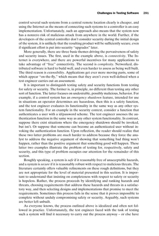
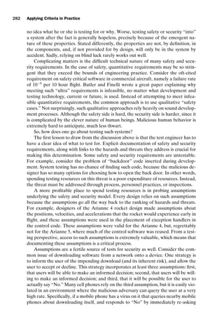
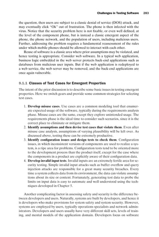
![introtest CUUS047-Ammann ISBN 9780521880381 November 8, 2007 17:13 Char Count= 0
Challenges in Testing Software 285
Notice that we do not specify what a fault at a given location necessarily looks
like. The reader might think it helpful to think of either average case or worst case
behavior for all faults possible at that location. The testability of an artifact is defined
as the minimum value of the sensitivity over all locations in the artifact.
To clarify the idea that sensitivities are probabilities, it is necessary to model in-
puts as being drawn from one or more usage distributions. In other words, we assume
that test cases are sampled from some profile. In practice, defining usage distribu-
tions is quite easy to do, and such an approach to testing has numerous proponents;
citations are available in the bibliographic notes section.
Given a distribution for selecting test inputs, measuring the reachability proba-
bility for any given location is a direct affair. Further, if the reachability probability
for a given location is deemed to be too low, it is easy to change the input distri-
bution to channel a larger fraction of the test inputs to that location. Stated more
directly, the reachability attribute of testability is under the direct control of the test
engineer. One way to think of this property is in terms of controllability. Software
with low controllability will probably suffer from low reachability probabilities, no
matter how the input distribution is skewed.
Estimating infection probabilities is a bit trickier, since it requires the adoption
of both a fault model and an infection model, both of which must be suitable for the
location in question. One choice is to use mutation analysis for the fault model, and
measure infections by observing the effect of mutants on candidate program states.
Determining propagation probabilities also involves a certain amount of mod-
eling. One choice is to use perturbation models to alter the program state at the
location in question and then observe whether the infection persists to the outputs.
One way to think of this property is in terms of observability. Software with low
observability will probably suffer from low propagation. However, there are quite a
few things that can be done to re-engineer code to have higher propagation.
First, there is the dimensionality of the output space to consider. For example,
consider a method with a single boolean output. Such a method is prone to have low
testability, if, for no other reason, than propagation from any infection is limited
by the collapsing of the entire internal state to a single boolean output. The test
engineer can interact with system designers to see if additional outputs are possible,
thereby giving better access to the internal state, and hence better propagation.
Second, there is the notion of assertion checking. Assertion mechanisms are
ideal for transforming internal state inconsistencies into observable events, typically
via an exception mechanism. Designers can assist this process by providing exten-
sive checks of internal states. Such checks need not be enabled during operational
deployment; from the testability perspective, it is sufficient that they be enabled
during testing only.
9.2.1 Testability for Common Technologies
Object-oriented software presents special challenges for testability. The chief rea-
son is that objects encode state information in instance variables, and access to these
instance variables is usually indirect. Consider the simple example of a stack. The
method push(Object item) changes the state of the stack, perhaps by storing item in
an instance variable Object[] elements. The method top() yields access to the most](https://image.slidesharecdn.com/introductiontosoftwaretesting-221201191322-f16668ac/85/Introduction-to-Software-Testing-pdf-309-320.jpg)
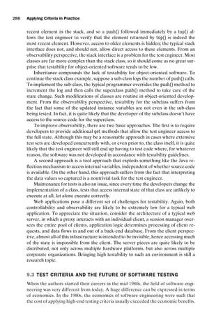
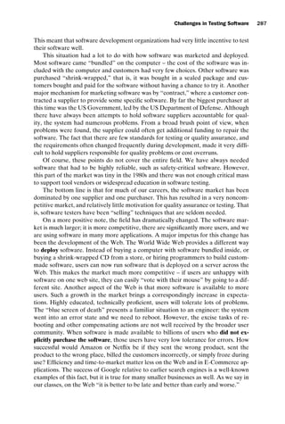
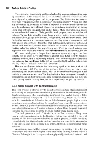
![introtest CUUS047-Ammann ISBN 9780521880381 November 8, 2007 17:13 Char Count= 0
290 Applying Criteria in Practice
in software testing focused on automatic test data generation, but progress proved
so difficult that most researchers diverted into more tractable problems. Some early
work focused on randomly generating test inputs. While simpler to implement than
other approaches, random test data generation has two problems. The first is that,
as Dick Lipton said, “faults ain’t fish.” That is, faults are not distributed uniformly
(randomly) through the program like fish in a school. Any programmer knows that
faults tend to clump around troublesome portions of the program or difficult to
define regions in the input space. The second problem with random test data gener-
ation is with structure data. It is easy to randomly generate numbers and characters,
but when the data has some structure (addresses, product records, etc.), random
generation becomes much harder.
The most complicated idea is to analyze program source and use detailed infor-
mation about the software to automatically generate test data specifically to satisfy
test criteria. The most common analysis method has been symbolic evaluation, often
coupled with constraint representations and sometimes slicing. Some analysis tech-
niques have been static and others dynamic. Solving the equations or constraints for
actual input values has been done with exact solutions such as constraint solving (lin-
ear programming) and inexact special purpose heuristics. Significant problems with
analysis-based techniques are the so-called “internal variable problem,” loops, and
indeterminate memory references such as pointers, arrays and aliases. The internal
variable problem refers to the fact that we may have specific requirements on test
inputs such as “X must be greater than Y on line 5306,” yet X and Y are not inputs.
Finding input values to indirectly control the values of X and Y has been trouble-
some. Dynamic analysis techniques are the most promising way to address these
problems, however, these problems are why analysis-based techniques are mostly
considered to apply to small structures such as program units.
The most recent automatic test data generation approach uses search techniques
such as genetic algorithms. Search-based approaches have several advantages, in-
cluding being easy to implement and being very flexible. They cannot use as much
information as the analysis-based methods, and thus can get stuck on values that
are hard to find. For example, if a search-based technique is used to achieve edge
coverage on a method-level control flow graph, a predicate such as x+y = z presents
difficulty for search-based techniques. This problem is compounded if several such
predicates have to be satisfied to reach a portion of the method. For this reason,
search-based techniques have so far achieved more success at the system level than
the unit level.
9.4 BIBLIOGRAPHIC NOTES
An excellent, if slightly dated, place to start on software for safety critical systems
is Leveson’s book [207]. Butler and Finelli wrote a great article on the futility of
assuring ultra high confidence levels in software via any means, including testing
[59]. Heimdahl [155] presents a good state-of-the-art perspective on the challenges
of safety in software intensive systems. McGraw [233] is a good current source for
the many issues to consider in building secure software. For a somewhat older treat-
ment, readers might wish to try Rubin [306]. Denning’s book [103] is a classic, al-
though it is out of print and hence harder to obtain.](https://image.slidesharecdn.com/introductiontosoftwaretesting-221201191322-f16668ac/85/Introduction-to-Software-Testing-pdf-314-320.jpg)
![introtest CUUS047-Ammann ISBN 9780521880381 November 8, 2007 17:13 Char Count= 0
Challenges in Testing Software 291
Casting the testability problem in terms of controllability and observability
comes originally from hardware testing; Friedman [129] and Binder [34] adapted it
to software testing. Voas [333] developed the three part sensitivity model described
in this chapter. Applying the testability model in conduction with random testing
yields an interesting verification argument [334].
Other criteria that we chose to omit are cataloged in a recent book by Pezze and
Young [289]. Other references can be found in the research papers cited in previous
chapters.
A good start for how the Web changes the way software is viewed is a book by
Powell [292]. Several authors have commented on the inadequacies of subsumption
for practical use [149, 340, 344]. We know of four papers that compared data flow
with mutation testing [125, 230, 267, 274]. Lots of other papers have appeared that
empirically compared other test criteria [25, 49, 81, 123, 124, 135, 258, 302, 304, 311,
327].
Random automatic test data generation approaches date back to the mid-1970s
[36, 176, 218, 243]. Older specification-based test data generation approaches use
formal specifications [23, 76]; more recent approaches use model-based languages
such as the UML [2, 46, 70]. Grammar-based test data generation approaches ap-
peared more than 35 years ago and are currently being revived for XML-based
software such as web services [150, 231, 248, 280]. Several researchers investi-
gated how to use program analysis techniques for automatic test data generation
[39, 80, 101, 102, 174, 190, 191, 267, 295, 342]. The use of search-based techniques,
primarily genetic algorithms started with informally acquiring knowledge about
tests [351] and has been refined since then [179, 234, 242].](https://image.slidesharecdn.com/introductiontosoftwaretesting-221201191322-f16668ac/85/Introduction-to-Software-Testing-pdf-315-320.jpg)

![introtest CUUS047-Ammann ISBN 9780521880381 November 21, 2007 18:48 Char Count= 0
Bibliography
[1] W3C #28. Extensible markup language (XML) 1.0 (second edition) – W3C rec-
ommendation, October 2000. http://www.w3.org/XML/#9802xml10.
[2] Aynur Abdurazik and Jeff Offutt. Using UML collaboration diagrams for static
checking and test generation. In Third International Conference on the Unified
Modeling Language (UML ’00), pages 383–395, York, England, October 2000.
[3] Aynur Abdurazik and Jeff Offutt. Coupling-based class integration and test or-
der. In Workshop on Automation of Software Test (AST 2006), pages 50–56,
Shanghai, China, May 2006.
[4] Alan T. Acree. On Mutation. PhD thesis, Georgia Institute of Technology, At-
lanta, GA, 1980.
[5] Alan T. Acree, Tim A. Budd, Richard A. DeMillo, Richard J. Lipton, and
Fred G. Sayward. Mutation analysis. Technical report GIT-ICS-79/08, School of
Information and Computer Science, Georgia Institute of Technology, Atlanta,
GA, September 1979.
[6] S. B. Akers. On a theory of boolean functions. Journal Society Industrial Applied
Mathematics, 7(4):487–498, December 1959.
[7] Roger T. Alexander. Testing the Polymorphic Relationships of Object-oriented
Programs. PhD thesis, George Mason University, Fairfax, VA, 2001. Technical
report ISE-TR-01-04, http://www.ise.gmu.edu/techrep/.
[8] Roger T. Alexander, James M. Bieman, Sudipto Chosh, and Bixia Ji. Mutation of
Java objects. In 13th International Symposium on Software Reliability Engineer-
ing, pages 341–351, Annapolis, MD, November 2002. IEEE Computer Society
Press.
[9] Roger T. Alexander, James M. Bieman, and John Viega. Coping with Java pro-
gramming stress. IEEE Computer, 33(4):30–38, 2000.
[10] Roger T. Alexander and Jeff Offutt. Analysis techniques for testing polymorphic
relationships. In Thirtieth International Conference on Technology of Object-
Oriented Languages and Systems (TOOLS USA ’99), pages 104–114, Santa Bar-
bara, CA, August 1999.
295](https://image.slidesharecdn.com/introductiontosoftwaretesting-221201191322-f16668ac/85/Introduction-to-Software-Testing-pdf-319-320.jpg)
![introtest CUUS047-Ammann ISBN 9780521880381 November 21, 2007 18:48 Char Count= 0
296 Bibliography
[11] Roger T. Alexander and Jeff Offutt. Criteria for testing polymorphic relation-
ships. In 11th International Symposium on Software Reliability Engineering,
pages 15–23, San Jose, CA, October 2000. IEEE Computer Society Press.
[12] Roger T. Alexander and Jeff Offutt. Coupling-based testing of O-O programs.
Journal of Universal Computer Science, 10(4):391–427, April 2004. http://www.
jucs.org/jucs 10 4/coupling based testing of.
[13] F. E. Allen and J. Cocke. A program data flow analysis procedure. Communica-
tions of the ACM, 19(3):137–146, March 1976.
[14] Paul Ammann and Paul Black. A specification-based coverage metric to evalu-
ate tests. In 4th IEEE International Symposium on High-Assurance Systems En-
gineering, pages 239–248, Washington, DC, November 1999.
[15] Paul Ammann, Paul Black, and W. Majurski. Using model checking to generate
tests from specifications. In 2nd International Conference on Formal Engineering
Methods, pages 46–54, Brisbane, Australia, December 1998.
[16] Paul Ammann and Jeff Offutt. Using formal methods to derive test frames in
category-partition testing. In Ninth Annual Conference on Computer Assurance
(COMPASS 94), pages 69–80, Gaithersburg MD, June 1994. IEEE Computer
Society Press.
[17] Paul Ammann, Jeff Offutt, and Hong Huang. Coverage criteria for logical ex-
pressions. In 14th International Symposium on Software Reliability Engineer-
ing, pages 99–107, Denver, CO, November 2003. IEEE Computer Society
Press.
[18] Paul E. Ammann and John C. Knight. Data diversity: An approach to software
fault tolerance. IEEE Transactions on Computers, 37(4):418–425, April 1988.
[19] D. M. St. Andre. Pilot mutation system (PIMS) user’s manual. Technical report
GIT-ICS-79/04, Georgia Institute of Technology, April 1979.
[20] Jo M. Atlee. Native model-checking of SCR requirements. In Fourth Interna-
tional SCR Workshop, November 1994.
[21] Jo M. Atlee and John Gannon. State-based model checking of event-driven
system requirements. IEEE Transactions on Software Engineering, 19(1):24–40,
January 1993.
[22] Algirdas Avizienis. The n-version approach to fault-tolerant software. IEEE
Transactions on Software Engineering, SE-11(12):1491–1501, December 1985.
[23] M. Balcer, W. Hasling, and T. Ostrand. Automatic generation of test scripts from
formal test specifications. In Third Symposium on Software Testing, Analysis, and
Verification, pages 210–218, Key West Florida, December 1989. ACM SIGSOFT
89.
[24] Stephane Barbey and Alfred Strohmeier. The problematics of testing object-
oriented software. In SQM’94 Second Conference on Software Quality
Management, volume 2, pages 411–426, Edinburgh, Scotland, UK, 1994.
[25] Vic R. Basili and Richard W. Selby. Comparing the effectiveness of software test-
ing strategies. IEEE Transactions on Software Engineering, 13(12):1278–1296,
December 1987.
[26] J. A. Bauer and A. B. Finger. Test plan generation using formal grammars. In
Fourth International Conference on Software Engineering, pages 425–432, Mu-
nich, September 1979.](https://image.slidesharecdn.com/introductiontosoftwaretesting-221201191322-f16668ac/85/Introduction-to-Software-Testing-pdf-320-320.jpg)
![introtest CUUS047-Ammann ISBN 9780521880381 November 21, 2007 18:48 Char Count= 0
Bibliography 297
[27] Erich Beck and Kent Gamma. JUnit: A cook’s tour. Java Report, 4(5):27–38,
May 1999.
[28] Boris Beizer. Software System Testing and Quality Assurance. Van Nostrand,
New York, 1984.
[29] Boris Beizer. Software Testing Techniques. Van Nostrand Reinhold, New York,
2nd edition, 1990. ISBN 0-442-20672-0.
[30] Michael Benedikt, Juliana Freire, and Patrice Godefroid. VeriWeb: Automat-
ically testing dynamic Web sites. In 11th International World Wide Web Con-
ference (WWW’2002) – Alternate Paper Tracks (WE-3 Web Testing and Mainte-
nance), pages 654–668, Honolulu, HI, May 2002.
[31] Edward V. Berard. Essays on Object-Oriented Software Engineering, volume 1.
Prentice Hall, New York, 1993.
[32] Philip J. Bernhard. A reduced test suite for protocol conformance testing. ACM
Transactions on Software Engineering and Methodology, 3(3):201–220, July 1994.
[33] Robert Binder. Testing Object-oriented Systems. Addison-Wesley, New York,
2000.
[34] Robert V. Binder. Design for testability in object-oriented systems. Communi-
cations of the ACM, 37(9):87–101, September 1994.
[35] Robert V. Binder. Testing object-oriented software: A survey. Software Testing,
Verification and Reliability, 6(3/4):125–252, 1996.
[36] D. L. Bird and C. U. Munoz. Automatic generation of random self-checking test
cases. IBM Systems Journal, 22(3):229–345, 1983.
[37] Paul Black, Vladim Okun, and Y. Yesha. Mutation operators for specifications.
In Fifteenth IEEE International Conference on Automated Software Engineering,
pages 81–88, September 2000.
[38] Manuel Blum and Sampath Kannan. Designing programs that check their work.
In Twenty-First ACM Symposium on the Theory of Computing, pages 86–97,
1989.
[39] Juris Borzovs, Audris Kalniņš, and Inga Medvedis. Automatic construction of
test sets: Practical approach. In Lecture Notes in Computer Science, Vol. 502,
pages 360–432. Springer Verlag, 1991.
[40] John H. Bowser. Reference manual for Ada mutant operators. Technical report
GIT-SERC-88/02, Georgia Institute of Technology, February 1988.
[41] R. S. Boyer, B. Elpas, and K. N. Levitt. Select – a formal system for testing and
debugging programs by symbolic execution. In International Conference on Reli-
able Software, June 1975. SIGPLAN Notices, vol. 10, no. 6.
[42] V. Braberman, M. Felder, and M. Marré. Testing timing behavior of real-time
software. In International Software Quality Week, 1997.
[43] T. Bray, J. Paoli, and C. M. Sperberg-McQueen. Extensible markup lan-
guage (XML) 1.0. W3C recommendation, February 1998. http://www.w3.org/
TR/REC-xml/.
[44] Lionel Briand, J. Feng, and Yvan Labiche. Using genetic algorithms and cou-
pling measures to devise optimal integration test orders. In 14th International
Conference on Software Engineering and Knowledge Engineering, pages 43–50,
Ischia, Italy, 2002. IEEE Computer Society Press.](https://image.slidesharecdn.com/introductiontosoftwaretesting-221201191322-f16668ac/85/Introduction-to-Software-Testing-pdf-321-320.jpg)
![introtest CUUS047-Ammann ISBN 9780521880381 November 21, 2007 18:48 Char Count= 0
298 Bibliography
[45] Lionel Briand and Yvan Labiche. A UML-based approach to system testing. In
Fourth International Conference on the Unified Modeling Language (UML ’01),
pages 194–208, Toronto, Canada, October 2001.
[46] Lionel Briand and Yvan Labiche. A UML-based approach to system testing.
Software and Systems Modeling, 1(1):10–42, 2002.
[47] Lionel Briand, Yvan Labiche, and Yihong Wang. Revisiting strategies for or-
dering class integration testing in the presence of dependency cycles. Technical
report sce-01-02, Careleton University, 2001.
[48] Lionel Briand, Yvan Labiche, and Yihong Wang. An investigation of graph-
based class integration test order strategies. IEEE Transactions on Software En-
gineering, 29(7):594–607, July 2003.
[49] Lionel Briand, Massimiliano Di Penta, and Y. Labiche. Assessing and improving
state-based class testing: A series of experiments. IEEE Transactions on Software
Engineering, 30(11):770–793, November 2004.
[50] R. Brownlie, J. Prowse, and M. S. Phadke. Robust testing of ATT PMX/
StarMAIL using OATS. ATT Technical Journal, 71(3):41–47, May/June 1992.
[51] Tim Budd and Dana Angluin. Two notions of correctness and their relation to
testing. Acta Informatica, 18(1):31–45, November 1982.
[52] Tim Budd and Fred Sayward. Users guide to the Pilot mutation system. Techni-
cal report 114, Department of Computer Science, Yale University, 1977.
[53] Tim A. Budd. Mutation Analysis of Program Test Data. PhD thesis, Yale Uni-
versity, New Haven, CT, 1980.
[54] Tim A. Budd, Richard A. DeMillo, Richard J. Lipton, and Fred G. Sayward.
The design of a prototype mutation system for program testing. In NCC, AFIPS
Conference Record, pages 623–627, 1978.
[55] Tim A. Budd and Richard J. Lipton. Proving Lisp programs using test data. In
Digest for the Workshop on Software Testing and Test Documentation, pages 374–
403, Ft. Lauderdale, FL, December 1978. IEEE Computer Society Press.
[56] Tim A. Budd, Richard J. Lipton, Richard A. DeMillo, and Fred G. Sayward.
Mutation analysis. Technical report GIT-ICS-79/08, School of Information and
Computer Science, Georgia Institute of Technology, Atlanta GA, April 1979.
[57] K. Burr and W. Young. Combinatorial test techniques: Table-based automation,
test generation and code coverage. In International Conference on Software Test-
ing, Analysis, and Review (STAR’98), San Diego, CA, October 1998.
[58] K. Burroughs, A. Jain, and R. L. Erickson. Improved quality of protocol testing
through techniques of experimental design. In IEEE International Conference on
Communications (Supercomm/ICC’94), pages 745–752, New Orleans, LA, May
1994. IEEE Computer Society Press.
[59] Ricky W. Butler and George B. Finelli. The infeasibility of quantifying the relia-
bility of life-critical real-time software. Software Engineering, 19(1):3–12, 1993.
[60] Ugo Buy, Alessandro Orso, and Mauro Pezze. Automated testing of classes. In
2000 International Symposium on Software Testing, and Analysis (ISSTA ’00),
pages 39–48, Portland, OR, August 2000. IEEE Computer Society Press.
[61] R. Cardell-Oliver and T. Glover. A practical and complete algorithm for testing
real-time systems. Lecture Notes in Computer Science, 1486:251–261, 1998.](https://image.slidesharecdn.com/introductiontosoftwaretesting-221201191322-f16668ac/85/Introduction-to-Software-Testing-pdf-322-320.jpg)
![introtest CUUS047-Ammann ISBN 9780521880381 November 21, 2007 18:48 Char Count= 0
Bibliography 299
[62] T. E. Cheatham, G. H. Holloway, and J. A. Townley. Symbolic evaluation and
the analysis of programs. IEEE Transactions on Software Engineering, 5(4), July
1979.
[63] T. Y. Chen and M. F. Lau. Test case selection strategies based on boolean
specifications. Software Testing, Verification, and Reliability, 11(3):165–180, June
2001.
[64] T. Y. Chen, P. L. Poon, S. F. Tang, and T. H. Tse. On the identification of cate-
gories and choices for specification-based test case generation. Information and
Software Technology, 46(13):887–898, 2004.
[65] T. Y. Chen, S. F. Tang, P. L. Poon, and T. H. Tse. Identification of categories and
choices in activity diagrams. In Fifth International Conference on Quality Soft-
ware (QSIC 2005), pages 55–63, Melbourne, Australia, September 2005. IEEE
Computer Society Press.
[66] J. C. Cherniavsky. On finding test data sets for loop free programs. Information
Processing Letters, 8(2):106–107, February 1979.
[67] J. C. Cherniavsky and C. H. Smith. A theory of program testing with applications.
Workshop on Software Testing, pages 110–121, July 1986.
[68] Shing Chi Cheung, Samuel T. Chanson, and Zhendong Xu. Toward generic tim-
ing tests for distributed multimedia software systems. In 12th International Sym-
posium on Software Reliability Engineering (ISSRE’01), page 210, Washington,
DC, 2001. IEEE Computer Society Press.
[69] Philippe Chevalley. Applying mutation analysis for object-oriented programs us-
ing a reflective approach. In 8th Asia-Pacific Software Engineering Conference
(APSEC 2001), Macau SAR, China, December 2001.
[70] Philippe Chevalley and Pascale Thévenod-Fosse. Automated generation of sta-
tistical test cases from UML state diagrams. In Proc. of IEEE 25th Annual In-
ternational Computer Software and Applications Conference (COMPSAC2001),
Chicago, IL, October 2001.
[71] Philippe Chevalley and Pascale Thévenod-Fosse. A mutation analysis tool for
Java programs. Journal on Software Tools for Technology Transfer (STTT),
September 2002.
[72] John J. Chilenski. Personal communication, March 2003.
[73] John J. Chilenski and Steven P. Miller. Applicability of modified condition/
decision coverage to software testing. Software Engineering Journal, 9(5):193–
200, September 1994.
[74] John J. Chilenski and L. A. Richey. Definition for a masking form of modified
condition decision coverage (MCDC). Technical report, Boeing, Seattle, WA,
1997.
[75] Byoung-Ju Choi and Aditya Mathur. High-performance mutation testing. Jour-
nal of Systems and Software, 20(2):135–152, February 1993.
[76] N. Choquet. Test data generation using a prolog with constraints. In Workshop
on Software Testing, pages 51–60, Banff, Alberta, July 1986. IEEE Computer
Society Press.
[77] T. Chow. Testing software designs modeled by finite-state machines. IEEE
Transactions on Software Engineering, SE-4(3):178–187, May 1978.](https://image.slidesharecdn.com/introductiontosoftwaretesting-221201191322-f16668ac/85/Introduction-to-Software-Testing-pdf-323-320.jpg)
![introtest CUUS047-Ammann ISBN 9780521880381 November 21, 2007 18:48 Char Count= 0
300 Bibliography
[78] D. Clarke and I. Lee. Automatic generation of tests for timing constraints from
requirements. In Third International Workshop on Object-Oriented Real-Time
Dependable Systems, Newport Beach, CA, February 1997.
[79] James M. Clarke. Automated test generation from a behavioral model. In Soft-
ware Quality Week Conference, Brussels, Belgium, May 1998.
[80] Lori Clarke. A system to generate test data and symbolically execute pro-
grams. IEEE Transactions on Software Engineering, 2(3):215–222, September
1976.
[81] Lori Clarke, Andy Podgurski, Debra Richardson, and Steven Zeil. A comparison
of data flow path selection criteria. In Eighth International Conference on Soft-
ware Engineering, pages 244–251, London, UK, August 1985. IEEE Computer
Society Press.
[82] Lori Clarke, Andy Podgurski, Debra Richardson, and Steven Zeil. A formal
evaluation of data flow path selection criteria. IEEE Transactions on Software
Engineering, 15:1318–1332, November 1989.
[83] Lori Clarke and Debra Richardson. Applications of symbolic evaluation. Journal
of Systems and Software, 5(1):15–35, January 1985.
[84] David M. Cohen, Siddhartha R. Dalal, Michael L. Fredman, and Gardner C. Pat-
ton. The AETG system: An approach to testing based on combinatorial design.
IEEE Transactions on Software Engineering, 23(7):437–444, July 1997.
[85] David M. Cohen, Siddhartha R. Dalal, A. Kajla, and Gardner C. Patton. The
automatic efficient test generator (AETG) system. In Fifth International Sympo-
sium on Software Reliability Engineering (ISSRE’94), pages 303–309, Los Alami-
tos, CA, November 1994. IEEE Computer Society Press.
[86] David M. Cohen, Siddhartha R. Dalal, Jesse Parelius, and Gardner C. Patton.
The combinatorial design approach to automatic test generation. IEEE Software,
pages 83–88, September 1996.
[87] M. B. Cohen, P. B. Gibbons, W. B. Mugridge, and C. J. Colburn. Constructing
test cases for interaction testing. In 25th International Conference on Software
Engineering, (ICSE’03), pages 38–48. IEEE Computer Society, May 2003.
[88] L. L. Constantine and E. Yourdon. Structured Design. Prentice-Hall, Englewood
Cliffs, NJ, 1979.
[89] Alan Cooper. About Face: The Essentials of User Interface Design. Hungry
Minds, New York, 1995.
[90] Lee Copeland. A Practitioner’s Guide to Software Test Design. Artech House
Publishers, Norwood, MA, 2003.
[91] S. R. Dalal, A. Jain, N. Karunanithi, J. M. Leaton, and C. M. Lott. Model-based
testing of a highly programmable system. In 9th International Symposium in Soft-
ware Engineering (ISSRE’98), pages 174–178, Paderborn, Germany, November
1998. IEEE Computer Society Press.
[92] S. R. Dalal, A. Jain, N. Karunanithi, J. M. Leaton, C. M. Lott, G. C. Patton, and
B. M. Horowitz. Model-based testing in practice. In 21st International Conference
on Software Engineering (ICSE’99), pages 285–294, Los Angeles, CA, May 1999.
ACM Press.
[93] J. A. Darringer and J. C. King. Applications of symbolic execution to program
testing. IEEE Computer, 11(4), April 1978.](https://image.slidesharecdn.com/introductiontosoftwaretesting-221201191322-f16668ac/85/Introduction-to-Software-Testing-pdf-324-320.jpg)
![introtest CUUS047-Ammann ISBN 9780521880381 November 21, 2007 18:48 Char Count= 0
Bibliography 301
[94] Márcio Delamaro, José C. Maldonado, and Aditya P. Mathur. Interface muta-
tion: An approach for integration testing. IEEE Transactions on Software Engi-
neering, 27(3):228–247, March 2001.
[95] Márcio E. Delamaro and José C. Maldonado. Proteum – A tool for the assess-
ment of test adequacy for C programs. In Conference on Performability in Com-
puting Systems (PCS 96), pages 79–95, New Brunswick, NJ, July 1996.
[96] Richard A. DeMillo, Dana S. Guindi, Kim N. King, W. Michael McCracken,
and Jeff Offutt. An extended overview of the Mothra software testing en-
vironment. In Second Workshop on Software Testing, Verification, and Anal-
ysis, pages 142–151, Banff, Alberta, July 1988. IEEE Computer Society
Press.
[97] Richard A. DeMillo, Edward Krauser, and Aditya P. Mathur. Compiler-
integrated program mutation. In Fifteenth Annual Computer Software and Appli-
cations Conference (COMPSAC ’92), Tokyo, Japan, September 1991. Kogakuin
University, IEEE Computer Society Press.
[98] Richard A. DeMillo, Richard J. Lipton, and Alan J. Perlis. Social processes and
proofs of theorems and programs. Communications of the ACM, 22(5), May
1979.
[99] Richard A. DeMillo, Richard J. Lipton, and Fred G. Sayward. Hints on test data
selection: Help for the practicing programmer. IEEE Computer, 11(4):34–41,
April 1978.
[100] Richard A. DeMillo, W. Michael McCracken, Rhonda J. Martin, and John F.
Passafiume. Software Testing and Evaluation. Benjamin/Cummings, Menlo Park,
CA, 1987.
[101] Richard A. DeMillo and Jeff Offutt. Constraint-based automatic test data gen-
eration. IEEE Transactions on Software Engineering, 17(9):900–910, September
1991.
[102] Richard A. DeMillo and Jeff Offutt. Experimental results from an automatic
test case generator. ACM Transactions on Software Engineering Methodology,
2(2):109–127, April 1993.
[103] Dorothy Denning. Cryptography and Data Security. Addison Wesley, New York,
1982.
[104] M. S. Deutsch. Software Verification and Validation Realistic Project Approaches.
Prentice-Hall, Englewood Cliffs, NJ, 1982.
[105] R. K. Doong and Phyllis G. Frankl. Case studies on testing object-oriented pro-
grams. In Fourth Symposium on Software Testing, Analysis, and Verification,
pages 165–177, Victoria, British Columbia, Canada, October 1991. IEEE Com-
puter Society Press.
[106] Mehmet S
. ahinoğlu and Eugene H. Spafford. A Bayes sequential statistical
procedure for approving software products. In Wolfgang Ehrenberger, editor,
The IFIP Conference on Approving Software Products (ASP–90), pages 43–56,
Garmisch-Partenkirchen, Germany, September 1990. Elsevier/North Holland,
New York.
[107] A. G. Duncan and J. S. Hutchison. Using attributed grammars to test designs
and implementations. In Fifth International Conference on Software Engineering,
pages 170–178, San Diego, CA, March 1981.](https://image.slidesharecdn.com/introductiontosoftwaretesting-221201191322-f16668ac/85/Introduction-to-Software-Testing-pdf-325-320.jpg)
![introtest CUUS047-Ammann ISBN 9780521880381 November 21, 2007 18:48 Char Count= 0
302 Bibliography
[108] Arnaud Dupuy and Nancy Leveson. An empirical evaluation of the MC/DC cov-
erage criterion on the HETE-2 satellite software. In Digital Aviations Systems
Conference (DASC), October 2000.
[109] Elfriede Dustin, Jeff Rashka, and John Paul. Automated Software Testing: In-
troduction, Management, and Performance. Addison-Wesley Professional, New
York, 1999.
[110] Dave E. Eckhardt Jr. and Larry D. Lee. Fundamental differences in the relia-
bility of n-modular redundancy and n-version programming. Journal of Systems
and Software, 8(4):313–318, September 1988.
[111] Alan Edelman. The mathematics of the Pentium division bug. SIAM Review,
39:54–67, March 1997. http://www.siam.org/journals/sirev/39-1/29395.html.
[112] Sebastian Elbaum, Srikanth Karre, and Gregg Rothermel. Improving Web ap-
plication testing with user session data. In 25th International Conference on Soft-
ware Engineering, pages 49–59, Portland, OR, May 2003. IEEE Computer Soci-
ety Press.
[113] Sebastian Elbaum, Gregg Rothermel, Srikanth Karre, and Marc Fisher. Lever-
aging user-session data to support web application testing. IEEE Transactions
on Software Engineering, 31(3):187–202, March 2005.
[114] R. En-Nouaary, Khendek F. Dssouli, and A. Elqortobi. Timed test case genera-
tion based on a state characterization technique. In Proceeding of the 19th IEEE
Real-Time Systems Symposium (RTSS98), Madrid, Spain, December 1998.
[115] Sadik Esmelioglu and Larry Apfelbaum. Automated test generation, execution,
and reporting. In Pacific Northwest Software Quality Conference. IEEE Press,
October 1997.
[116] R. E. Fairley. An experimental program testing facility. IEEE Transactions on
Software Engineering, SE-1:350–3571, December 1975.
[117] Roger Ferguson and Bogdan Korel. The chaining approach for software test data
generation. ACM Transactions on Software Engineering Methodology, 5(1):63–
86, January 1996.
[118] S. P. Fiedler. Object-oriented unit testing. Hewlett-Packard Journal, 40(2):69–74,
April 1989.
[119] Donald G. Firesmith. Testing object-oriented software. In Testing Object-
Oriented Languages and Systems (TOOLS), March 1993.
[120] Vladimir N. Fleyshgakker and Stewart N. Weiss. Efficient mutation analysis: A
new approach. In International Symposium on Software Testing and Analysis
(ISSTA 94), pages 185–195, Seattle, WA, August 17–19 1994. ACM SIGSOFT,
ACM Press.
[121] I. R. Forman. An algebra for data flow anomaly detection. In Seventh Interna-
tional Conference on Software Engineering, pages 278–286. Orlando, FL, March
1984. IEEE Computer Society Press.
[122] L. D. Fosdick and L. J. Osterweil. Data flow analysis in software reliability. ACM
Computing Surveys, 8(3):305–330, September 1976.
[123] Phyllis G. Frankl and Yuetang Deng. Comparison of delivered reliability of
branch, data flow and operational testing: A case study. In 2000 International
Symposium on Software Testing, and Analysis (ISSTA ’00), pages 124–134, Port-
land, OR, August 2000. IEEE Computer Society Press.](https://image.slidesharecdn.com/introductiontosoftwaretesting-221201191322-f16668ac/85/Introduction-to-Software-Testing-pdf-326-320.jpg)
![introtest CUUS047-Ammann ISBN 9780521880381 November 21, 2007 18:48 Char Count= 0
Bibliography 303
[124] Phyllis G. Frankl and Stewart N. Weiss. An experimental comparison of the ef-
fectiveness of branch testing and data flow testing. IEEE Transactions on Soft-
ware Engineering, 19(8):774–787, August 1993.
[125] Phyllis G. Frankl, Stewart N. Weiss, and C. Hu. All-uses versus mutation testing:
An experimental comparison of effectiveness. Journal of Systems and Software,
38(3):235–253, 1997.
[126] Phyllis G. Frankl, Stewart N. Weiss, and Elaine J. Weyuker. ASSET: A system
to select and evaluate tests. In Conference on Software Tools, New York, April
1985. IEEE Computer Society Press.
[127] Phyllis G. Frankl and Elaine J. Weyuker. Data flow testing in the presence of un-
executable paths. In Workshop on Software Testing, pages 4–13, Banff, Alberta,
July 1986. IEEE Computer Society Press.
[128] Phyllis G. Frankl and Elaine J. Weyuker. An applicable family of data flow test-
ing criteria. IEEE Transactions on Software Engineering, 14(10):1483–1498, Oc-
tober 1988.
[129] Roy S. Freedman. Testability of software components. IEEE Transactions on
Software Engineering, 17(6):553–564, June 1991.
[130] S. Fujiwara, G. Bochman, F. Khendek, M. Amalou, and A. Ghedasmi. Test se-
lection based on finite state models. IEEE Transactions on Software Engineering,
17(6):591–603, June 1991.
[131] J. Gait. A probe effect in concurrent programs. Software – Practice and Experi-
ence, 16(3):225–233, March 1986.
[132] Leonard Gallagher, Jeff Offutt, and Tony Cincotta. Integration testing of object-
oriented components using finite state machines. Software Testing, Verification,
and Reliability, 17(1):215–266, January 2007.
[133] Robert Geist, Jeff Offutt, and Fred Harris. Estimation and enhancement of real-
time software reliability through mutation analysis. IEEE Transactions on Com-
puters, 41(5):550–558, May 1992. Special issue on Fault-Tolerant Computing.
[134] M. R. Girgis and M. R. Woodward. An integrated system for program testing
using weak mutation and data flow analysis. In Eighth International Conference
on Software Engineering, pages 313–319, London, UK, August 1985. IEEE Com-
puter Society Press.
[135] M. R. Girgis and M. R. Woodward. An experimental comparison of the error
exposing ability of program testing criteria. In Workshop on Software Testing,
pages 64–73. Banff, Canada, July 1986. IEEE Computer Society Press.
[136] A. Goldberg, T. C. Wang, and D. Zimmerman. Applications of feasible path
analysis to program testing. In 1994 International Symposium on Software Test-
ing, and Analysis, pages 80–94, Seattle, WA, August 1994.
[137] G. Gonenc. A method for the design of fault-detection experiments. IEEE
Transactions on Computers, C-19:155–558, June 1970.
[138] J. B. Goodenough and S. L. Gerhart. Toward a theory of test data selection.
IEEE Transactions on Software Engineering, 1(2), June 1975.
[139] J. S. Gourlay. A mathematical framework for the investigation of testing. IEEE
Transactions on Software Engineering, 9(6):686–709, November 1983.
[140] Mats Grindal. Evaluation of Combination Strategies for Practical Testing. PhD
thesis, Skövde University / Linköping University, Skövde Sweden, 2007.](https://image.slidesharecdn.com/introductiontosoftwaretesting-221201191322-f16668ac/85/Introduction-to-Software-Testing-pdf-327-320.jpg)
![introtest CUUS047-Ammann ISBN 9780521880381 November 21, 2007 18:48 Char Count= 0
304 Bibliography
[141] Mats Grindal, Birgitta Lindström, Jeff Offutt, and Sten F. Andler. An evaluation
of combination testing strategies. Empirical Software Engineering, 11(4):583–
611, December 2006.
[142] Mats Grindal and Jeff Offutt. Input parameter modeling for combination strate-
gies. In IASTED International Conference on Software Engineering (SE 2007),
Innsbruck, Austria, February 2007. ACTA Press.
[143] Mats Grindal, Jeff Offutt, and Sten F. Andler. Combination testing strategies: A
survey. Software Testing, Verification, and Reliability, 15(2):97–133, September
2005.
[144] Mats Grindal, Jeff Offutt, and Jonas Mellin. Conflict management when us-
ing combination strategies for software testing. In Australian Software Engi-
neering Conference (ASWEC 2007), pages 255–264, Melbourne, Australia, April
2007.
[145] Matthias Grochtmann and Klaus Grimm. Classification trees for partition test-
ing. Software Testing, Verification, and Reliability, 3(2):63–82, 1993.
[146] Matthias Grochtmann, Klaus Grimm, and J. Wegener. Tool-supported test case
design for black-box testing by means of the classification-tree editor. In 1st Eu-
ropean International Conference on Software Testing Analysis Review (Eu-
roSTAR 1993), pages 169–176, London, UK, October 1993.
[147] Richard Hamlet. Reliability theory of program testing. Acta Informatica, pages
31–43, 1981.
[148] Richard G. Hamlet. Testing programs with the aid of a compiler. IEEE Transac-
tions on Software Engineering, 3(4):279–290, July 1977.
[149] Richard G. Hamlet and Richard Taylor. Partition testing does not inspire confi-
dence. IEEE Transactions on Software Engineering, 16(12):1402–1411, Decem-
ber 1990.
[150] K. V. Hanford. Automatic generation of test cases. IBM Systems Journal, 4:242–
257, 1970.
[151] Jim M. Hanks. Testing cobol programs by mutation: Volume I – Introduction to
the CMS.1 system, Volume II – CMS.1 system documentation. Technical report
GIT-ICS-80/04, Georgia Institute of Technology, February 1980.
[152] Mary Jean Harrold and Gregg Rothermel. Performing data flow testing on
classes. In Symposium on Foundations of Software Engineering, pages 154–163,
New Orleans, LA, December 1994. ACM SIGSOFT.
[153] Mary Jean Harrold and Gregg Rothermel. Empirical studies of a safe regression
test selection technque. IEEE Transactions on Software Engineering, 24(6):401–
419, June 1998.
[154] Mary Jean Harrold and Mary Lou Soffa. Selecting and using data for integration
testing. IEEE Software, 8(2):58–65, March 1991.
[155] Mats E. Heimdahl. Safety and software intensive systems: Challenges old and
new. In International Conference on Software Engineering: Future of Software
Engineering, pages 137–152, May 2007.
[156] E. Heller. Using design of experiment structures to generate software test cases.
In 12th International Conference on Testing Computer Software, pages 33–41,
New York, 1995. ACM.](https://image.slidesharecdn.com/introductiontosoftwaretesting-221201191322-f16668ac/85/Introduction-to-Software-Testing-pdf-328-320.jpg)
![introtest CUUS047-Ammann ISBN 9780521880381 November 21, 2007 18:48 Char Count= 0
Bibliography 305
[157] K. Henninger. Specifiying software requirements for complex systems: New tech-
niques and their applications. IEEE Transactions on Software Engineering, SE-
6(1):2–12, January 1980.
[158] P. Herman. A data flow analysis approach to program testing. Australian Com-
puter Journal, 8(3):92–96, November 1976.
[159] A. Hessel, K. Larsen, B. Nielsen, and A Skou. Time optimal real-time test case
generation using UPPAAL. In Workshop on Formal Approaches to Testing of
Software (FATES), Montreal, October 2003.
[160] Bill Hetzel. The Complete Guide to Software Testing. Wiley-QED, second edi-
tion, 1988.
[161] J. Robert Horgan and Saul London. Data flow coverage and the C language.
In Fourth Symposium on Software Testing, Analysis, and Verification, pages 87–
97, Victoria, British Columbia, Canada, October 1991. IEEE Computer Society
Press.
[162] J. Robert Horgan and Saul London. ATAC: A data flow coverage testing tool
for C. In Symposium of Quality Software Development Tools, pages 2–10, New
Orleans, LA, May 1992. IEEE Computer Society Press.
[163] J. Robert Horgan and Aditya P. Mathur. Weak mutation is proba-
bly strong mutation. Technical report SERC-TR-83-P, Software Engineer-
ing Research Center, Purdue University, West Lafayette, IN, December
1990.
[164] Willam E. Howden. Methodology for the generation of program test data. IEEE
Transactions on Software Engineering, SE-24, May 1975.
[165] Willam E. Howden. Reliability of the path analysis testing strategy. IEEE Trans-
actions on Software Engineering, 2(3):208–215, September 1976.
[166] Willam E. Howden. Symbolic testing and the DISSECT symbolic evaluation sys-
tem. IEEE Transactions on Software Engineering, 3(4), July 1977.
[167] Willam E. Howden. Weak mutation testing and completeness of test sets. IEEE
Transactions on Software Engineering, 8(4):371–379, July 1982.
[168] Willam E. Howden. The theory and practice of function testing. IEEE Software,
2(5), September 1985.
[169] William E. Howden. Functional Program Testing and Analysis. McGraw-Hill,
New York, 1987.
[170] J. C. Huang. An approach to program testing. ACM Computing Surveys,
7(3):113–128, September 1975.
[171] J. Huller. Reducing time to market with combinatorial design method testing. In
10th Annual International Council on Systems Engineering (INCOSE’00), Min-
neapolis, MN, July 2000.
[172] M. Hutchins, H. Foster, T. Goradia, and T. Ostrand. Experiments on the
effectiveness of dataflow- and controlflow-based test adequacy criteria. In Six-
teenth International Conference on Software Engineering, pages 191–200, Sor-
rento, Italy, May 1994. IEEE Computer Society Press.
[173] Michael Huth and Mark D. Ryan. Logic in Computer Science: Modelling
and Reasoning About Systems. Cambridge University Press, Cambridge, UK,
2000.](https://image.slidesharecdn.com/introductiontosoftwaretesting-221201191322-f16668ac/85/Introduction-to-Software-Testing-pdf-329-320.jpg)
![introtest CUUS047-Ammann ISBN 9780521880381 November 21, 2007 18:48 Char Count= 0
306 Bibliography
[174] G. Hwang, K. Tai, and T. Hunag. Reachability testing: An approach to testing
concurrent software. International Journal of Software Engineering and Knowl-
edge Engineering, 5(4), December 1995.
[175] IEEE. IEEE Standard Glossary of Software Engineering Terminology. ANSI/
IEEE Std 610.12-1990, 1996.
[176] D. C. Ince. The automatic generation of test data. Computer Journal, 30(1):63–
69, 1987.
[177] R. Jasper, M. Brennan, K. Williamson, B. Currier, and D. Zimmerman. Test data
generation and feasible path analysis. In 1994 International Symposium on Soft-
ware Testing, and Analysis, pages 95–107, Seattle, WA, August 1994.
[178] Zhenyi Jin and Jeff Offutt. Coupling-based criteria for integration testing. Soft-
ware Testing, Verification, and Reliability, 8(3):133–154, September 1998.
[179] B. F. Jones, D. E. Eyres, and H. H. Sthamer. A strategy for using genetic algo-
rithms to automate branch and fault-based testing. Computer Journal, 41(2):98–
107, 1998.
[180] J. A. Jones and Mary Jean Harrold. Test-suite reduction and prioritizaion for
modified condition/decision coverage. IEEE Transactions on Software Engineer-
ing, 29(3):195–209, March 2003.
[181] Paul C. Jorgensen and Carl Erickson. Object-oriented integration testing. Com-
munications of the ACM, 37(9):30–38, 1994.
[182] Cem Kaner, Jack Falk, and Hung Q. Nguyen. Testing Computer Software. John
Wiley and Sons, New York NY, second edition, 1999.
[183] David J. Kasik and Harry G. George. Toward automatic generation of novice
user test scripts. In Conference on Human Factors in Computing Systems: Com-
mon Ground, pages 244–251, New York, April 1996.
[184] Sun-Woo Kim, John Clark, and John McDermid. Assessing test set adequacy
for object-oriented programs using class mutation. In of Symposium on Software
Technology (SoST’99), pages 72–83, September 1999.
[185] Sunwoo Kim, John A. Clark, and John A. McDermid. Investigating the effective-
ness of object-oriented strategies with the mutation method. In Mutation 2000:
Mutation Testing in the Twentieth and the Twenty First Centuries, pages 4–100,
San Jose, CA, October 2000. Special issue of the Journal of Software Testing,
Verification, and Reliability, December 2001.
[186] Y. G. Kim, H. S. Hong, S. M. Cho, D. H. Bae, and S. D. Cha. Test cases gen-
eration from UML state diagrams. IEE Proceedings – Software, 146(4):187–192,
August 1999.
[187] Kim N. King and Jeff Offutt. A Fortran language system for mutation-based
software testing. Software – Practice and Experience, 21(7):685–718, July 1991.
[188] John C. Knight and Nancy G. Leveson. An experimental evaluation of the as-
sumption of independence in multiversion programming. IEEE Transactions on
Software Engineering, SE-12(1):96–109, January 1986.
[189] Charles Knutson and Sam Carmichael. Safety first: Avoiding software mishaps,
November 2000. http://www.embedded.com/2000/0011/0011feat1.htm.
[190] Bogdan Korel. Automated software test data generation. IEEE Transactions on
Software Engineering, 16(8):870–879, August 1990.](https://image.slidesharecdn.com/introductiontosoftwaretesting-221201191322-f16668ac/85/Introduction-to-Software-Testing-pdf-330-320.jpg)
![introtest CUUS047-Ammann ISBN 9780521880381 November 21, 2007 18:48 Char Count= 0
Bibliography 307
[191] Bogdan Korel. Dynamic method for software test data generation. Software Test-
ing, Verification, and Reliability, 2(4):203–213, 1992.
[192] Edward W. Krauser, Aditya P. Mathur, and Vernon Rego. High performance
testing on SIMD machines. In Second Workshop on Software Testing, Verifica-
tion, and Analysis, pages 171–177, Banff, Alberta, July 1988. IEEE Computer
Society Press.
[193] M. Krichen and S. Tripakis. Black-box conformance testing for real-time sys-
tems. In The SPIN’04 Workshop on Model-Checking Software, Barcelona, Spain,
2004.
[194] D. R. Kuhn. Fault classes and error detection capability of specification-based
testing. ACM Transactions on Software Engineering Methodology, 8(4):411–424,
October 1999.
[195] D. R. Kuhn and M. J. Reilly. An investigation of the applicability of design
of experiments to software testing. In 27th NASA/IEE Software Engineering
Workshop, NASA Goodard Space Flight Center, MD, December 2002. NASA/
IEEE.
[196] D. R. Kuhn, D. R. Wallace, and A. M. Gallo Jr. Software fault interactions and
implications for software testing. IEEE Transactions on Software Engineering,
30(6):418–421, June 2004.
[197] D. Kung, J. Gao, Pei Hsia, Y. Toyoshima, and C. Chen. A test strategy for
object-oriented programs. In 19th Computer Software and Applications Confer-
ence (COMPSAC ’95), pages 239–244, Dallas, TX, August 1995. IEEE Com-
puter Society Press.
[198] D. Kung, C. H. Liu, and P. Hsia. An object-oriented Web test model for testing
Web applications. In IEEE 24th Annual International Computer Software and
Applications Conference (COMPSAC2000), pages 537–542, Taipei, Taiwan, Oc-
tober 2000.
[199] W. LaLonde and J. Pugh. Subclassing != subtyping != is-a. Journal of Object
Oriented Programming, 3(5): 57–62, January 1991.
[200] Janusz Laski. Data flow testing in STAD. Journal of Systems and Software, 12:3–
14, 1990.
[201] Janusz Laski and Bogdan Korel. A data flow oriented program testing strategy.
IEEE Transactions on Software Engineering, 9(3):347–354, May 1983.
[202] M. F. Lau and Y. T. Yu. An extended fault class hierarchy for specification-based
testing. ACM Transactions on Software Engineering Methodology, 14(3):247–
276, July 2005.
[203] Suet Chun Lee and Jeff Offutt. Generating test cases for XML-based web com-
ponent interactions using mutation analysis. In 12th International Symposium on
Software Reliability Engineering, pages 200–209, Hong Kong, China, November
2001. IEEE Computer Society Press.
[204] H. Legard and M. Marcotty. A generalogy of control structures. Communications
of the ACM, 18:629–639, November 1975.
[205] Yu Lei and K. C. Tai. In-parameter-order: A test generation strategy for pair-
wise testing. In Third IEEE High Assurance Systems Engineering Symposium,
pages 254–261, November 1998. IEEE Computer Society Press.](https://image.slidesharecdn.com/introductiontosoftwaretesting-221201191322-f16668ac/85/Introduction-to-Software-Testing-pdf-331-320.jpg)
![introtest CUUS047-Ammann ISBN 9780521880381 November 21, 2007 18:48 Char Count= 0
308 Bibliography
[206] Yu Lei and K. C. Tai. A test generation strategy for pairwise testing. Techni-
cal Report TR-2001-03, Department of Computer Science, North Carolina State
University, Raleigh, 2001.
[207] Nancy G. Leveson. Safeware: System Safety and Computers. Addison-Wesley,
Reading, MA, 1995.
[208] Zhang Li, Mark Harman, and Rob M. Hierons. Meta-heuristic search algorithms
for regression test case prioritization. IEEE Transactions on Software Engineer-
ing, 33(4):225–237, April 2007.
[209] J. L. Lions. Ariane 5 flight 501 failure: Report by the inquiry board, July 1996.
http://sunnyday.mit.edu/accidents/Ariane5accidentreport.html.
[210] Richard Lipton. New directions in testing. In Distributed Computing and Cryp-
tography, DIMACS Series in Discrete Mathematics and Theoretical Computer
Science, volume 2, pages 191–202, Providence, RI, 1991.
[211] Richard J. Lipton and Fred G. Sayward. The status of research on program mu-
tation. In Digest for the Workshop on Software Testing and Test Documentation,
pages 355–373, December 1978.
[212] Barbara Liskov and John Guttag. Program Development in Java: Abstraction,
Specification, and Object-Oriented Design. Addison Wesley, New York, 2000.
[213] Barbara H. Liskov and Jeannette M. Wing. A behavioral notion of subtyping.
ACM Transactions on Programming Languages and Systems, 16(1):1811–1841,
November 1994.
[214] B. Littlewood and D. R. Miller. Conceptual modeling of coincident fail-
ures in multiversion software. IEEE Transactions on Software Engineering,
15(12):1596–1614, December 1989.
[215] C. H. Liu, D. Kung, P. Hsia, and C. T. Hsu. Structural testing of Web appli-
cations. In 11th International Symposium on Software Reliability Engineering,
pages 84–96, San Jose, CA, October 2000. IEEE Computer Society Press.
[216] C. H. Liu, D. C. Kung, P. Hsia, and C. T. Hsu. An object-based data flow testing
approach for Web applications. International Journal of Software Engineering
and Knowledge Engineering, 11(2):157–179, 2001.
[217] Giuseppe A. Di Lucca and Massimiliano Di Penta. Considering browser interac-
tion in web application testing. In 5th International Workshop on Web Site Evo-
lution (WSE 2003), pages 74–84, Amsterdam, The Netherlands, September 2003.
IEEE Computer Society Press.
[218] Stephen F. Lundstrom. Adaptive random data generation for computer software
testing. In National Computer Conference, pages 505–511, 1978.
[219] Yu-Seung Ma, Yong-Rae Kwon, and Jeff Offutt. Inter-class mutation operators
for Java. In 13th International Symposium on Software Reliability Engineering,
pages 352–363, Annapolis, MD, November 2002. IEEE Computer Society Press.
[220] Yu-Seung Ma, Jeff Offutt, and Yong-Rae Kwon. Mujava : An automated class
mutation system. Software Testing, Verification, and Reliability, 15(2):97–133,
June 2005.
[221] Yu-Seung Ma, Jeff Offutt, and Yong-Rae Kwon. mujava home page. online,
2005. http://ise.gmu.edu/ offutt/mujava/, http://salmosa.kaist.ac.kr/LAB/MuJava/,
last access April 2006.](https://image.slidesharecdn.com/introductiontosoftwaretesting-221201191322-f16668ac/85/Introduction-to-Software-Testing-pdf-332-320.jpg)
![introtest CUUS047-Ammann ISBN 9780521880381 November 21, 2007 18:48 Char Count= 0
Bibliography 309
[222] Yashwant K. Malaiya. Antirandom testing: Getting the most out of black-box
testing. In International Symposium on Software Reliability Engineering (IS-
SRE’95), pages 86–95, Toulouse, France, October 1995.
[223] Brian A. Malloy, Peter J. Clarke, and Errol L. Lloyd. A parameterized cost
model to order classes for class-based testing of C++ applications. In 14th In-
ternational Symposium on Software Reliability Engineering, Denver, CO, 2003.
IEEE Computer Society Press.
[224] Robert Mandl. Orthogonal latin squares: An application of experiment design
to compiler testing. Communications of the ACM, 28(10):1054–1058, October
1985.
[225] D. Mandrioli, S. Morasca, and A. Morzenti. Generating test cases for real-
time systems from logic specifications. ACM Transactions on Computer Systems,
4(13):365–398, Nov. 1995.
[226] Brian Marick. The weak mutation hypothesis. In Fourth Symposium on Software
Testing, Analysis, and Verification, pages 190–199, Victoria, British Columbia,
Canada, October 1991. IEEE Computer Society Press.
[227] Brian Marick. The Craft of Software Testing: Subsystem Testing, Including
Object-Based and Object-Oriented Testing. Prentice-Hall, Englewood Cliffs,
New Jersey, 1995.
[228] Aditya P. Mathur. On the relative strengths of data flow and mutation based test
adequacy criteria. In Sixth Annual Pacific Northwest Software Quality Confer-
ence, Portland, OR, Lawrence and Craig, 1991.
[229] Aditya P. Mathur and Edward W. Krauser. Mutant unification for improved
vectorization. Technical report SERC-TR-14-P, Software Engineering Research
Center, Purdue University, West Lafayette, IN, April 1988.
[230] Aditya P. Mathur and W. Eric Wong. An empirical comparison of data flow and
mutation-based test adequacy criteria. Software Testing, Verification, and Relia-
bility, 4(1):9–31, March 1994.
[231] P. M. Maurer. Generating test data with enhanced context-free grammars. IEEE
Software, 7(4):50–55, July 1990.
[232] T. J. McCabe. A complexity measure. IEEE Transactions on Software Engineer-
ing, 2(4):308–320, December 1976.
[233] Gary McGraw. Software Security: Building Security In. Addison-Wesley, New
York, 2006.
[234] Phil McMinn. Search-based software test data generation: A survey. Software
Testing, Verification, and Reliability, 13(2):105–156, June 2004.
[235] Atif M. Memon, Martha E. Pollack, and Mary Lou Soffa. Using a goal-driven
approach to generate test cases for GUIs. In 21st International Conference on
Software Engineering, pages 257–266, May 1999.
[236] Atif M. Memon, Martha E. Pollack, and Mary Lou Soffa. Automated test oracles
for GUIs. In ACM SIGSOFT 8th International Symposium on the Foundations
of Software Engineering (FSE-8), pages 30–39, New York, November 2000.
[237] Atif M. Memon, Martha E. Pollack, and Mary Lou Soffa. Hierarchical GUI test
case generation using automated planning. IEEE Transactions on Software En-
gineering, 27(2):144–155, February 2001.](https://image.slidesharecdn.com/introductiontosoftwaretesting-221201191322-f16668ac/85/Introduction-to-Software-Testing-pdf-333-320.jpg)
![introtest CUUS047-Ammann ISBN 9780521880381 November 21, 2007 18:48 Char Count= 0
310 Bibliography
[238] Atif M. Memon and Mary Lou Soffa. Regression testing of GUIs. In 9th Eu-
ropean Software Engineering Conference (ESEC) and 11th ACM SIGSOFT In-
ternational Symposium on the Foundations of Software Engineering (FSE-11),
pages 118–127, September 2003.
[239] Atif M. Memon, Mary Lou Soffa, and Martha E. Pollack. Coverage criteria for
GUI testing. In 8th European Software Engineering Conference (ESEC) and 9th
ACM SIGSOFT International Symposium on the Foundations of Software Engi-
neering (FSE-9), pages 256–267, September 2001.
[240] Atif M. Memon and Qing Xie. Empirical evaluation of the fault-detection ef-
fectiveness of smoke regression test cases for GUI-based software. In The In-
ternational Conference on Software Maintenance 2004 (ICSM’04), pages 8–17,
Washington, DC, September 2004.
[241] Bertrand Meyer. Object-Oriented Software Construction. Prentice Hall, Upper
Saddle River, NJ, second edition, 1997.
[242] C. C. Michael, G. McGraw, and M. A. Schatz. Generating software test data by
evolution. IEEE Transactions on Software Engineering, 27(12):1085–1110, De-
cember 2001.
[243] E. F. Miller and R. A. Melton. Automated generation of testcase datasets. In
International Conference on Reliable Software, pages 51–58, April 1975.
[244] Cleve Moler. A tale of two numbers. SIAM News, 28(1), January 1995.
[245] S. Morasca and Mauro Pezze. Using high level Petri-nets for testing concurrent
and real-time systems. Real-Time Systems: Theory and Applications, pages 119–
131. Amsterdam, North-Holland, 1990.
[246] Larry J. Morell. A Theory of Error-Based Testing. PhD thesis, University of
Maryland, College Park, MD, 1984. Technical Report TR-1395.
[247] Larry J. Morell. A theory of fault-based testing. IEEE Transactions on Software
Engineering, 16(8):844–857, August 1990.
[248] Carlos Urias Munoz. An approach to software product testing. IEEE Transac-
tions on Software Engineering, 14(11):1589–1595, November 1988.
[249] Glenford Myers. The Art of Software Testing. John Wiley and Sons, New York,
1979.
[250] Adithya Nagarajan and Atif M. Memon. Refactoring using event-based profil-
ing. In First International Workshop on REFactoring: Achievements, Challenges,
Effects (REFACE), Victoria, British Columbia, November 2003.
[251] S. Naito and M. Tsunoyama. Fault detection for sequential machines by transi-
tion tours. In Fault Tolerant Computing Systems, pages 238–243. IEEE Computer
Society Press, 1981.
[252] B. Nielsen and A. Skou. Automated test generation from timed automata. In
21st IEEE Real-Time Systems Symposium, Walt Disney World, Orlando, FL,
2000. IEEE Computer Society Press.
[253] Jacok Nielsen. Designing Web Usability. New Riders Publishing, Indianapolis,
IN, 2000.
[254] Robert Nilsson. Automatic Timeliness Testing of Dynamic Real-Time Sys-
tems. PhD thesis, Skövde University/Linköping University, Skövde Sweden,
2006.](https://image.slidesharecdn.com/introductiontosoftwaretesting-221201191322-f16668ac/85/Introduction-to-Software-Testing-pdf-334-320.jpg)
![introtest CUUS047-Ammann ISBN 9780521880381 November 21, 2007 18:48 Char Count= 0
Bibliography 311
[255] Robert Nilsson and Jeff Offutt. Automated testing of timeliness : A case study.
In Second Workshop on Automation of Software Test (AST 2007), Minneapolis,
MN, May 2007.
[256] Robert Nilsson, Jeff Offutt, and Sten F. Andler. Mutation-based testing criteria
for timeliness. In 28th Annual International Computer Software and Applications
Conference (COMPSAC 2004), pages 306–312, Hong Kong, September 2004.
[257] Robert Nilsson, Jeff Offutt, and Jonas Mellin. Test case generation for mutation-
based testing of timeliness. In 2nd International Workshop on Model Based Test-
ing, pages 102–121, Vienna, Austria, March 2006.
[258] S. C. Ntafos. An evaluation of required element testing strategies. In Seventh
International Conference on Software Engineering, pages 250–256, Orlando FL,
March 1984. IEEE Computer Society Press.
[259] Bashar Nuseibeh. Who dunnit? IEEE Software, 14:15–16, May/June 1997.
[260] Department of Defense. DOD-STD-2167A: Defense System Software Develop-
ment. Department of Defense, February 1988.
[261] Department of Defense. MIL-STD-498: Software Development and Documenta-
tion. Department of Defense, December 1994.
[262] Jeff Offutt. Automatic Test Data Generation. PhD thesis, Georgia Institute of
Technology, Atlanta, GA, 1988. Technical report GIT-ICS 88/28.
[263] Jeff Offutt. Investigations of the software testing coupling effect. ACM Transac-
tions on Software Engineering Methodology, 1(1):3–18, January 1992.
[264] Jeff Offutt and Aynur Abdurazik. Generating tests from UML specifications.
In Second IEEE International Conference on the Unified Modeling Language
(UML99), pages 416–429, Fort Collins, CO, October 1999. Springer-Verlag Lec-
ture Notes in Computer Science Volume 1723.
[265] Jeff Offutt, Aynur Abdurazik, and Roger T. Alexander. An analysis tool for
coupling-based integration testing. In The Sixth IEEE International Conference
on Engineering of Complex Computer Systems (ICECCS ’00), pages 172–178,
Tokyo, Japan, September 2000. IEEE Computer Society Press.
[266] Jeff Offutt, Roger Alexander, Ye Wu, Quansheng Xiao, and Chuck Hutchin-
son. A fault model for subtype inheritance and polymorphism. In 12th Interna-
tional Symposium on Software Reliability Engineering, pages 84–93, Hong Kong,
China, November 2001. IEEE Computer Society Press.
[267] Jeff Offutt, Zhenyi Jin, and Jie Pan. The dynamic domain reduction approach to
test data generation. Software – Practice and Experience, 29(2):167–193, January
1999.
[268] Jeff Offutt and Kim N. King. A Fortran 77 interpreter for mutation analysis. In
1987 Symposium on Interpreters and Interpretive Techniques, pages 177–188, St.
Paul MN, June 1987. ACM SIGPLAN.
[269] Jeff Offutt, Ammei Lee, Gregg Rothermel, Roland Untch, and Christian Zapf.
An experimental determination of sufficient mutation operators. ACM Transac-
tions on Software Engineering Methodology, 5(2):99–118, April 1996.
[270] Jeff Offutt and Stephen D. Lee. How strong is weak mutation? In Fourth Sym-
posium on Software Testing, Analysis, and Verification, pages 200–213, Victoria,
British Columbia, Canada, October 1991. IEEE Computer Society Press.](https://image.slidesharecdn.com/introductiontosoftwaretesting-221201191322-f16668ac/85/Introduction-to-Software-Testing-pdf-335-320.jpg)
![introtest CUUS047-Ammann ISBN 9780521880381 November 21, 2007 18:48 Char Count= 0
312 Bibliography
[271] Jeff Offutt and Stephen D. Lee. An empirical evaluation of weak mutation.
IEEE Transactions on Software Engineering, 20(5):337–344, May 1994.
[272] Jeff Offutt, Shaoying Liu, Aynur Abdurazik, and Paul Ammann. Generating test
data from state-based specifications. Software Testing, Verification, and Reliabil-
ity, 13(1):25–53, March 2003.
[273] Jeff Offutt and Jie Pan. Detecting equivalent mutants and the feasible path
problem. Software Testing, Verification, and Reliability, 7(3):165–192, September
1997.
[274] Jeff Offutt, Jie Pan, Kanupriya Tewary, and Tong Zhang. An experimental eval-
uation of data flow and mutation testing. Software – Practice and Experience,
26(2):165–176, February 1996.
[275] Jeff Offutt, Roy Pargas, Scott V. Fichter, and P. Khambekar. Mutation testing of
software using a MIMD computer. In 1992 International Conference on Parallel
Processing, pages II257–266, Chicago, August 1992.
[276] Jeff Offutt, Jeffrey Payne, and Jeffrey M. Voas. Mutation operators for Ada.
Technical report ISSE-TR-96-09, Department of Information and Software
Systems Engineering, George Mason University, Fairfax, VA, March 1996.
http://www.ise.gmu.edu/techrep/.
[277] Jeff Offutt and Roland Untch. Mutation 2000: Uniting the orthogonal. In Muta-
tion 2000: Mutation Testing in the Twentieth and the Twenty First Centuries, pages
45–55, San Jose, CA, October 2000.
[278] Jeff Offutt, Ye Wu, Xiaochen Du, and Hong Huang. Bypass testing of web ap-
plications. In 15th International Symposium on Software Reliability Engineering,
pages 187–197, Saint-Malo, Bretagne, France, November 2004. IEEE Computer
Society Press.
[279] Jeff Offutt and Wuzhi Xu. Generating test cases for web services using data per-
turbation. In Workshop on Testing, Analysis and Verification of Web Services,
Boston, MA, July 2004. ACM SIGSoft.
[280] Jeff Offutt and Wuzhi Xu. Testing web services by XML perturbation. In 16th In-
ternational Symposium on Software Reliability Engineering, Chicago, IL, Novem-
ber 2005. IEEE Computer Society Press.
[281] Alex Orso and Mauro Pezze. Integration testing of procedural object oriented
programs with polymorphism. In Sixteenth International Conference on Testing
Computer Software, pages 103–114, Washington, DC, June 1999. ACM SIG-
SOFT.
[282] L. J. Osterweil and L. D. Fosdick. Data flow analysis as an aid in documentation,
assertion generation, validation, and error detection. Technical report CU-CS-
055-74, Department of Computer Science, University of Colorado, Boulder, CO,
September 1974.
[283] T. J. Ostrand and M. J. Balcer. The category-partition method for specifying and
generating functional tests. Communications of the ACM, 31(6):676–686, June
1988.
[284] Jan Overbeck. Integration Testing for Object-Oriented Software. PhD disserta-
tion, Vienna University of Technology, 1994.
[285] A. J. Payne. A formalised technique for expressing compiler exercisers.
SIGLPAN Notices, 13(1):59–69, January 1978.](https://image.slidesharecdn.com/introductiontosoftwaretesting-221201191322-f16668ac/85/Introduction-to-Software-Testing-pdf-336-320.jpg)
![introtest CUUS047-Ammann ISBN 9780521880381 November 21, 2007 18:48 Char Count= 0
Bibliography 313
[286] Ivars Peterson. Pentium bug revisited, May 1997. http://www.maa.org/mathland/
mathland 5 12.html.
[287] E. Petitjean and H. Fochal. A realistic architecture for timed testing. In Fifth
IEEE International Conference on Engineering of Complex Computer Systems,
Las Vegas, October 1999.
[288] A. Pettersson and H. Thane. Testing of multi-tasking real-time systems with
critical sections. In Proceedings of Ninth International Conference on Real-Time
Computing Systems and Applications (RTCSA’03), Tainan City, Taiwan, Febru-
ary 2003.
[289] Mauro Pezze and Michal Young. Software Testing and Analysis: Process, Princi-
ples, and Techniques. Wiley, Hoboken, NJ, 2008.
[290] S. Pimont and J. C. Rault. A software reliability assessment based on a structural
behavioral analysis of programs. In Second International Conference on Software
Engineering, San Francisco, CA, October 1976.
[291] P. Piwowarski, M. Ohba, and J. Caruso. Coverage measure experience dur-
ing function test. In 14th International Conference on Software Engineering
(ICSE’93), pages 287–301, Los Alamitos, CA, May 1993. ACM.
[292] T. A. Powell. Web Site Engineering: Beyond Web Page Design. Prentice-Hall,
Englewood Cliffs, NJ, 2000.
[293] R. E. Prather. Theory of program testing – an overview. Bell System Technical
Journal, 62(10):3073–3105, December 1983.
[294] Paul Purdom. A sentence generator for testing parsers. BIT, 12:366–375, 1972.
[295] C. V. Ramamoorthy, S. F. Ho, and W. T. Chen. On the automated generation
of program test data. IEEE Transactions on Software Engineering, 2(4):293–300,
December 1976.
[296] K. Ramamritham. The origin of time constraints. In First International Work-
shop on Active and Real-Time Database Systems (ARTDB 1995), pages 50–62,
Skövde, Sweden, June 1995. Springer, New York, 1995.
[297] S. Rapps and Elaine J. Weyuker. Selecting software test data using data flow
information. IEEE Transactions on Software Engineering, 11(4):367–375, April
1985.
[298] S. Rayadurgam and M. P. E. Heimdahl. Coverage based test-case genera-
tion using model checkers. In 8th IEEE International Conference and Work-
shop on the Engineering of Computer Based Systems, pages 83–91, April
2001.
[299] Pascal Raymond, Xavier Nicollin, Nicolas Halbwachs, and Daniel Weber. Au-
tomatic testing of reactive systems. In Proceeding of the 19th IEEE Real-Time
Systems Symposium (RTSS98), 1998.
[300] F. Ricca and P. Tonella. Analysis and testing of Web applications. In 23rd Inter-
national Conference on Software Engineering (ICSE ‘01), pages 25–34, Toronto,
CA, May 2001.
[301] Marc Roper. Software Testing. International Software Quality Assurance Series.
McGraw-Hill, New York, 1994.
[302] Dave Rosenblum and Gregg Rothermel. A comparative study of regression test
selection techniques. In IEEE Computer Society 2nd International Workshop on](https://image.slidesharecdn.com/introductiontosoftwaretesting-221201191322-f16668ac/85/Introduction-to-Software-Testing-pdf-337-320.jpg)
![introtest CUUS047-Ammann ISBN 9780521880381 November 21, 2007 18:48 Char Count= 0
314 Bibliography
Empirical Studies of Software Maintenance, pages 89–94, Bari, Italy, October
1997. IEEE Computer Society Press.
[303] Gregg Rothermel and Mary Jean Harrold. Analyzing regression test selection
techniques. IEEE Transactions on Software Engineering, 22(8):529–551, August
1996.
[304] J. Rowland and Y. Zuyuan. Experimental comparison of three system test strate-
gies preliminary report. In Third Symposium on Software Testing, Analysis, and
Verification, pages 141–149, Key West, FL, December 1989. ACM SIGSOFT 89.
[305] RTCA-DO-178B. Software considerations in airborne systems and equipment
certification, December 1992.
[306] Avi D. Rubin. White-Hat Secuirty Arsenal: Tackling the Threats. Addison-
Wesley, New York, 2001.
[307] K. Sabnani and A. Dahbura. A protocol testing procedure. Computer Networks
and ISDN Systems, 14(4):285–297, 1988.
[308] P. SanPietro, A. Morzenti, and S. Morasca. Generation of execution sequences
for modular time critical systems. IEEE Transactions on Software Engineering,
26(2):128–149, February 2000.
[309] W. Schütz. The Testability of Distributed Real-Time Systems. Kluwer Academic
Publishers, Norwell, MA, 1993.
[310] W. Schütz. Fundamental issues in testing distributed real-time systems. Real-
Time Systems, 7(2):129–157, September 1994.
[311] Richard W. Selby. Combining software testing strategies: An empirical evalua-
tion. In Workshop on Software Testing, pages 82–90, Banff, Alberta, July 1986.
IEEE Computer Society Press.
[312] Richard K. Shehady and Daniel P. Siewiorek. A method to automate user in-
terface testing using variable finite state machines. In 27th International Sympo-
sium on Fault-Tolerant Computing (FTCS’97), pages 80–88, Washington, Brus-
sels, Tokyo, June 1997.
[313] G. Sherwood. Effective testing of factor combinations. In Third International
Conference on Software Testing, Analysis, and Review (STAR94), Washington,
DC, May 1994. Software Quality Engineering.
[314] T. Shiba, T. Tsuchiya, and T. Kikuno. Using artificial life techniques to generate
test cases for combinatorial testing. In 28th Annual International Computer Soft-
ware and Applications Conference (COMPSAC’04), pages 72–77, Hong Kong,
China, September 2004. IEEE Computer Society Press.
[315] M. D. Smith and D. J. Robson. Object-oriented programming: The problems of
validation. In 6th International Conference on Software Maintenance, pages 272–
282, Los Alamitos, CA, 1990. IEEE Computer Society Press.
[316] Ian Sommerville. Software Engineering. Addison-Wesley, New York, 6th edi-
tion, 2001.
[317] British Computer Society Specialist Interest Group in Software Testing. Stan-
dard for Software Component Testing, Working Draft 3.3. British Computer So-
ciety, 1997. http://www.rmcs.cranfield.ac.uk/∼cised/sreid/BCS SIG/.
[318] W. P. Stevens, G. J. Myers, and L. L. Constantine. Structured design. IBM Sys-
tems Journal, 13(2):115–139, 1974.](https://image.slidesharecdn.com/introductiontosoftwaretesting-221201191322-f16668ac/85/Introduction-to-Software-Testing-pdf-338-320.jpg)
![introtest CUUS047-Ammann ISBN 9780521880381 November 21, 2007 18:48 Char Count= 0
Bibliography 315
[319] Phil Stocks and Dave Carrington. Test templates: A specification-based testing
framework. In Fifteenth International Conference on Software Engineering, pages
405–414, Baltimore, MD, May 1993.
[320] Phil Stocks and Dave Carrington. A framework for specification-based testing.
IEEE Transactions on Software Engineering, 22(11):777–793, November 1996.
[321] K. C. Tai and F. J. Daniels. Test order for inter-class integration testing of object-
oriented software. In The Twenty-First Annual International Computer Software
and Applications Conference (COMPSAC ’97), pages 602–607, Santa Barbara,
CA, 1997. IEEE Computer Society.
[322] K. C. Tai and Yu Lei. A test generation strategy for pairwise testing. IEEE
Transactions on Software Engineering, 28(1):109–111, January 2002.
[323] Antero Taivalsaari. On the notion of inheritance. ACM Computing Surveys,
28(3):438–479, September 1996.
[324] M. Tatsubori. OpenJava WWW page. Tokyo Institute of Technology, Chiba
Shigeru Group, 2002. http://www.csg.is.titech.ac.jp/∼mich/openjava/ (accessed
May 2004).
[325] M. Tatsubori, S. Chiba, M.-O. Killijian, and K. Itano. OpenJava: A class-based
macro system for Java. Reflection and Software Engineering, LNCS 1826:117–
133, June 2000.
[326] H. Thane. Monitoring, Testing and Debugging of Distributed Real-Time Systems.
PhD thesis, Royal Institute of Technology, KTH, Stockholm, Sweden, 2000.
[327] P. Thévenod-Fosse, H. Waeselynck, and Y. Crouzet. An experimental study
on software structural testing: Deterministic versus random input generation.
In Fault-Tolerant Computing: The Twenty-First International Symposium, pages
410–417, Montreal, Canada, June 1991. IEEE Computer Society Press.
[328] F. Tip. A survey of program slicing techniques. Technical report CS-R-
9438, Computer Science/Department of Software Technology, Centrum voor
Wiskunde en Informatica, 1994.
[329] Yves Le Traon, Thierry Jéron, Jean-Marc Jézéquel, and Pierre Morel. Efficient
object-oriented integration and regression testing. IEEE Transactions on Relia-
bility, 49(1):12–25, March 2000.
[330] Roland H. Untch, Jeff Offutt, and Mary Jean Harrold. Mutation analysis using
program schemata. In 1993 International Symposium on Software Testing, and
Analysis, pages 139–148, Cambridge, MA, June 1993.
[331] P. Verissimo and H. Kopetz. Design of distributed real-time systems. In S. Mul-
lender, editor, Distributed Systems, pages 511–530. Addison-Wesley, New York,
1993.
[332] S. A. Vilkomir and J. P. Bowen. Reinforced condition/decision coverage
(RC/DC): A new criterion for software testing. In ZB2002: 2nd International
Conference of Z and B Users, pages 295–313, Grenoble, France, January 2002.
Springer-Verlag, LNCS 2272.
[333] Jeffrey M. Voas. Pie: A dynamic failure-based technique. IEEE Transactions on
Software Engineering, 18(8):717–727, August 1992.
[334] Jeffrey M. Voas and Keith W. Miller. Software testability: The new verification.
IEEE Software, 12(3):553–563, May 1995.](https://image.slidesharecdn.com/introductiontosoftwaretesting-221201191322-f16668ac/85/Introduction-to-Software-Testing-pdf-339-320.jpg)
![introtest CUUS047-Ammann ISBN 9780521880381 November 21, 2007 18:48 Char Count= 0
316 Bibliography
[335] K. S. How Tai Wah. Fault coupling in finite bijective functions. Software Testing,
Verification, and Reliability, 5(1):3–47, March 1995.
[336] K. S. How Tai Wah. A theoretical study of fault coupling. Software Testing, Ver-
ification, and Reliability, 10(1):3–46, March 2000.
[337] A. Watkins, D. Berndt, K. Aebischer, J. Fisher, and L. Johnson. Breeding soft-
ware test cases for complex systems. In 37th Annual Hawaii International Confer-
ence on System Sciences (HICSS’04) – Track 9, page 90303.3, Washington, DC,
USA, 2004. IEEE Computer Society Press.
[338] J. Wegener, H. H. Sthammer, B. F. Jones, and D. E. Eyres. Testing real-time
systems using genetic algorithms. Software Quality Journal, 6(2):127–135, 1997.
[339] Mark Weiser. Program slicing. IEEE Transactions on Software Engineering, SE-
10(4):352–357, July 1984.
[340] Steward N. Weiss. What to compare when comparing test data adequacy criteria.
ACM SIGSOFT Notes, 14(6):42–49, October 1989.
[341] Elaine Weyuker. The oracle assumption of program testing. In Thirteenth
International Conference on System Sciences, pages 44–49, Honolulu, HI, Jan-
uary 1980.
[342] Elaine Weyuker, Thomas Goradia, and A. Singh. Automatically generating test
data from a boolean specification. IEEE Transactions on Software Engineering,
20(5):353–363, May 1994.
[343] Elaine J. Weyuker and Thomas J. Ostrand. Theories of program testing and the
application of revealing subdomains. IEEE Transactions on Software Engineer-
ing, 6(3):236–246, May 1980.
[344] Elaine J. Weyuker, Stewart N. Weiss, and Richard G. Hamlet. Comparison of
program testing strategies. In Fourth Symposium on Software Testing, Analysis,
and Verification, pages 1–10, Victoria, British Columbia, Canada, October 1991.
IEEE Computer Society Press.
[345] Elaine J. Weyuker, Stewart N. Weiss, and Richard G. Hamlet. Data flow-based
adequacy analysis for languages with pointers. In Fourth Symposium on Soft-
ware Testing, Analysis, and Verification, pages 74–86, Victoria, British Columbia,
Canada, October 1991. IEEE Computer Society Press.
[346] Lee White and Husain Almezen. Generating test cases for GUI responsibilities
using complete interaction sequences. In 9th International Symposium on Soft-
ware Reliability Engineering, pages 110–121, October 2000.
[347] Lee White, Husain Almezen, and Nasser Alzeidi. User-based testing of GUI
sequences and their interaction. In 10th International Symposium on Software
Reliability Engineering, pages 54–63, November 2001.
[348] Lee White and Bogdan Wiszniewski. Path testing of computer programs with
loops using a tool for simple loop patterns. Software – Practice and Experience,
21(10):1075–1102, October 1991.
[349] Lee J. White. Software testing and verification. In Marshall C. Yovits, editor,
Advances in Computers, volume 26, pages 335–390. Academic Press, New York,
1987.
[350] Duminda Wijesekera, Lingya Sun, Paul Ammann, and Gordon Fraser. Relating
counterexamples to test cases in CTL model checking specifications. In A-MOST](https://image.slidesharecdn.com/introductiontosoftwaretesting-221201191322-f16668ac/85/Introduction-to-Software-Testing-pdf-340-320.jpg)
![introtest CUUS047-Ammann ISBN 9780521880381 November 21, 2007 18:48 Char Count= 0
Bibliography 317
’07: Third ACM Workshop on the Advances in Model-Based Testing, co-located
with ISSTA 2007, London, UK, July 2007.
[351] Christian Wild, Steven Zeil, and Gao Feng. Employing accumulated knowledge
to refine test descriptions. Software Testing, Verification, and Reliability, July
2(2): 53–68, 1992.
[352] Alan W. Williams. Determination of test configurations for pair-wise interaction
coverage. In 13th International Conference on the Testing of Communicating Sys-
tems (TestCom 2000), pages 59–74, Ottawa, Canada, August 2000.
[353] Alan W. Williams and Robert L. Probert. A practical strategy for testing pair-
wise coverage of network interfaces. In 7th International Symposium on Software
Reliability Engineering (ISSRE96), White Plains, New York, November 1996.
[354] Alan W. Williams and Robert L. Probert. A measure for component interaction
test coverage. In ACSI/IEEE International Conference on Computer Systems and
Applications (AICCSA 2001), pages 304–311, Beirut, Lebanon, June 2001.
[355] Barbara Liskov with John Guttag. Program Development in Java: Abstraction,
Specification, and Object-Oriented Design. Addison-Wesley, New York, 2001.
[356] W. Eric Wong. On Mutation and Data Flow. PhD thesis, Purdue University, De-
cember 1993. (Also Technical Report SERC-TR-149-P, Software Engineering
Research Center, Purdue University, West Lafayette, IN).
[357] W. Eric Wong and Aditya P. Mathur. Fault detection effectiveness of mutation
and data flow testing. Software Quality Journal, 4(1):69–83, March 1995.
[358] M. R. Woodward and K. Halewood. From weak to strong, dead or alive? An
analysis of some mutation testing issues. In Second Workshop on Software Test-
ing, Verification, and Analysis, pages 152–158, Banff Alberta, July 1988. IEEE
Computer Society Press.
[359] Ye Wu and Jeff Offutt. Modeling and testing Web-based applications. Tech-
nical report ISE-TR-02-08, Department of Information and Software Engi-
neering, George Mason University, Fairfax, VA, July 2002. http://www.ise.
gmu.edu/techrep/.
[360] Ye Wu, Jeff Offutt, and Xiaochen Du. Modeling and testing of dynamic aspects
of Web applications. Technical report ISE-TR-04-01, Department of Informa-
tion and Software Engineering, George Mason University, Fairfax, VA, July
2004. http://www.ise.gmu.edu/techrep/.
[361] Tao Xie and Dave Notkin. Checking inside the black box: Regression test-
ing by comparing value spectra. IEEE Transactions on Software Engineering,
31(10):869–883, October 2005.
[362] C. Yilmaz, M. B. Cohen, and A. Porter. Covering arrays for efficient fault
characterization in complex configuration spaces. In ACM SIGSOFT Interna-
tional Symposium on Software Testing and Analysis (ISSTA 2004), pages 45–54,
Boston, MA, July 2004. ACM Software Engineering Notes.
[363] H. Yin, Z. Lebne-Dengel, and Y. K. Malaiya. Automatic test generation using
checkpoint encoding and antirandom testing. Technical Report CS-97-116, Col-
orado State University, 1997.
[364] S. J. Young. Real-Time Languages: Design and Development. Ellis Horwood,
Chichester, UK, 1982.](https://image.slidesharecdn.com/introductiontosoftwaretesting-221201191322-f16668ac/85/Introduction-to-Software-Testing-pdf-341-320.jpg)
![introtest CUUS047-Ammann ISBN 9780521880381 November 21, 2007 18:48 Char Count= 0
318 Bibliography
[365] Christian N. Zapf. Medusamothra – A distributed interpreter for the mothra
mutation testing system. M.S. thesis, Clemson University, Clemson, SC, August
1993.
[366] Hong Zhu. A formal analysis of the subsume relation between software test ade-
quacy criteria. IEEE Transactions on Software Engineering, 22(4):248–255, April
1996.
[367] Hong Zhu, Patrick A. V. Hall, and John H. R. May. Software unit test coverage
and adequacy. ACM Computing Surveys, 29(4):366–427, December 1997.](https://image.slidesharecdn.com/introductiontosoftwaretesting-221201191322-f16668ac/85/Introduction-to-Software-Testing-pdf-342-320.jpg)


![30 February 2005 QUEUE rants [email protected] DARNEDTestin.docx](https://cdn.slidesharecdn.com/ss_thumbnails/30february2005queuerantsemailprotecteddarnedtestin-221107145618-9187028b-thumbnail.jpg?width=640&height=640&fit=bounds)


