This document provides an introduction to MATLAB, a high-performance computing language, including its environment, operators, and functions for handling variables, vectors, and matrices. It includes examples of matrix operations and mathematical functions, as well as instructions for 2D plotting. The course will utilize Piazza for Q&A and covers essential MATLAB topics through various examples and explanations.


![Vectors And Matrices
• In MATLAB matrices are easy to define:
• Use ‘ ’ to separate row elements.
• Use ‘;’ to separate rows.
>> y = [1 2 3; 4 5 6; 7 8 9]
y =
1 2 3
4 5 6
7 8 9](https://image.slidesharecdn.com/intro1-181208165618/75/Introduction-to-MATLAB-1-11-2048.jpg)
![Vectors And Matrices
• Order of Matrix
◦m = no. of rows.
◦n = no. of columns.
• Vectors are special case
m = 1 row vector n = 1 column vector
A =
0.9501 0.6068 0.4231
0.2311 0.4860 0.2774m
n
>> x = [1 2 3 4]
x =
1 2 3 4
>> x = [1; 2; 3; 4]
x =
1
2
3
4](https://image.slidesharecdn.com/intro1-181208165618/75/Introduction-to-MATLAB-1-12-2048.jpg)
![Long Vector, Matrix
>> x = 1:10
x =
1 2 3 4 5 6 7 8 9 10
>> x = 1:0.5:5
x =
1 1.5 2 2.5 3 3.5 4 4.5 5
>> [1:4; 5:8]
x =
1 2 3 4
5 6 7 8
• If you want to create a row
vector, containing numbers
from 1 to 10, you write
• If you want to specify an
increment value other than
one, for example
• Also you can create a matrix
using the colon.](https://image.slidesharecdn.com/intro1-181208165618/75/Introduction-to-MATLAB-1-13-2048.jpg)


![Concatenation of Matrices
>> x = [1 2]
x =
1 2
>> y = [3 4]
y =
3 4
>> A = [x y]
A =
1 2 3 4
>> B = [x; y]
B =
1 2
3 4
• Given:
• you can create a matrix or construct one from other matrices.](https://image.slidesharecdn.com/intro1-181208165618/75/Introduction-to-MATLAB-1-22-2048.jpg)
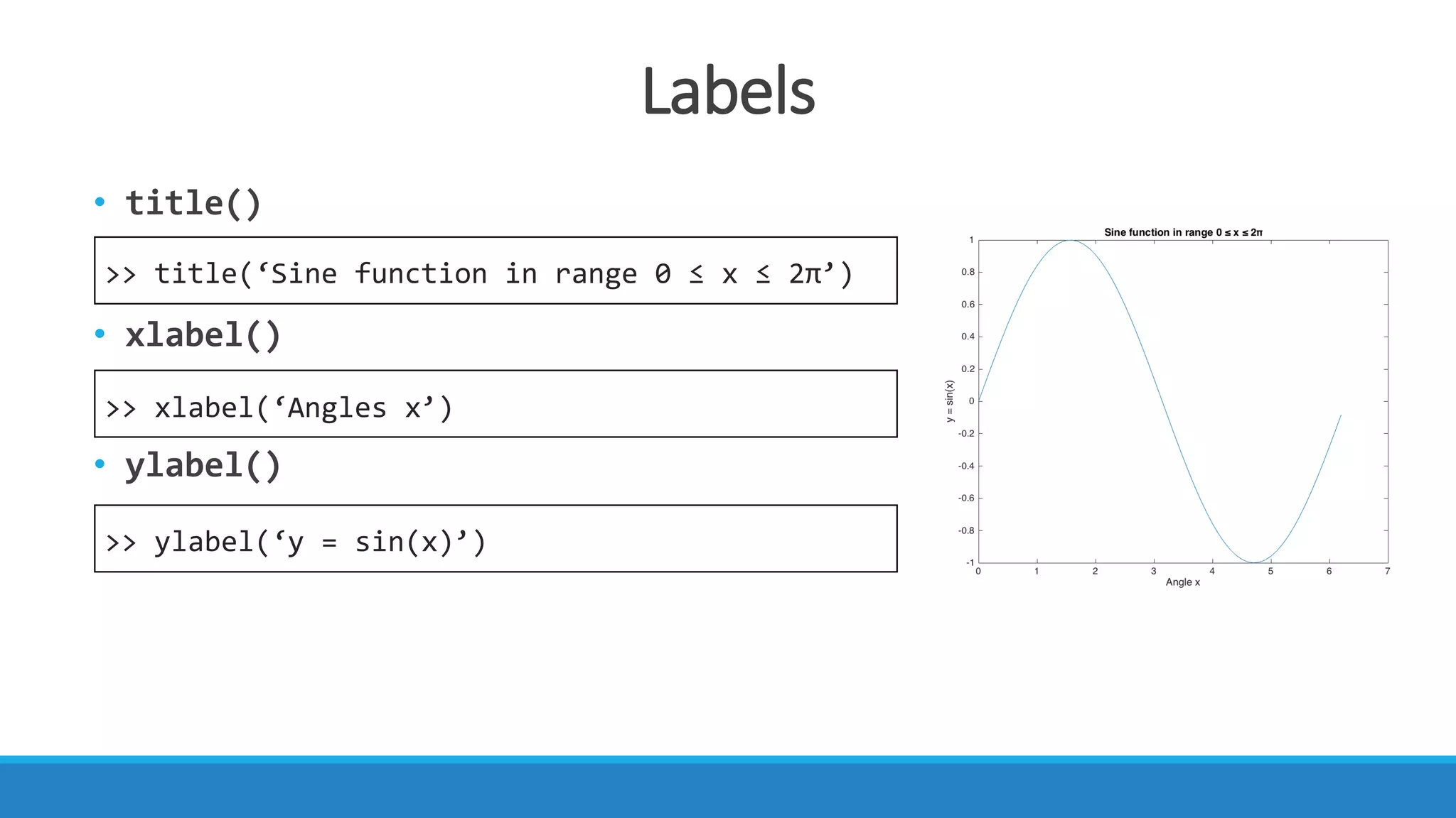
![2D Plotting In MATLAB
• Note:
• The semicolon(;) tells MATLAB not to
display any output from that command.
>> x = [0:0.1:2*pi];
>> y = sin(x);
>> plot(x, y)
Sine function in range 0 ≤ x ≤ 2π.
• We are going to plot the function sin(x) between 0 ≤ x ≤ 2π.
• First, we define the range of the independent variable, x to be between 0 and
2π. i.e. between 0 and 360.
• Then, we define the dependent variable,
y by writing the command y = sin(x).
• We plot using the function, plot(x,y).](https://image.slidesharecdn.com/intro1-181208165618/75/Introduction-to-MATLAB-1-27-2048.jpg)