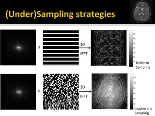
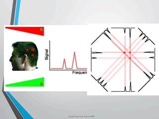
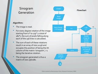
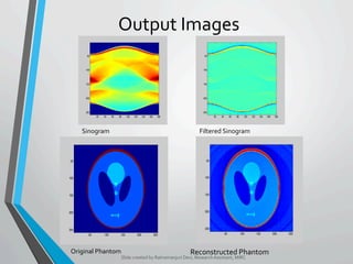
The document provides an overview of medical image processing, focusing on edge detection methods such as Sobel, Prewitt, Roberts, and the Canny edge detector, and discusses their implementation in MATLAB. It also covers image reconstruction using filtered back projection and the SENSE (Sensitivity Encoding) technique for parallel MRI imaging. The algorithms outlined include sinogram generation, image reconstruction strategies, and practical examples with MATLAB codes.

1. Ge#ng your feet wet with
Medical Image Processing
An overview of

2. Outline
• Digital image processing
– Basics of edge detec?on algorithms
• Medical image reconstruc?on
– Filtered backprojec?on for CT
– SENSE MRI reconstruc?on

3. EDGE DETECTION IN
MATLAB
Slide created by Ratnamanjuri Devi, Research Assistant, MIRC

4. INTRODUCTION
„ The abrupt changes or discontinuities in the intensity values in an image represent the
edges present in it.
„ Edge Detection is an approach used in Image Segmentation for detecting these edges.
„ These discontinuities are detected using first and second order derivatives
„ The first order derivative of choice is called the gradient.
„ The gradient of a 2D function f(x, y) (image) is defined by:
∇f = [Gx, Gy] = [∂f/∂x, ∂f/∂y]
where, Gx and Gy are gradients in the x and y direction respectively.
„ The gradient vector points in the direction of maximum rate of change, which are the
edges.
„ Second order derivatives are usually computed using the Laplacian method.
„ The Laplacian of a 2D function f(x,y) is defined by:
∇2f(x, y) = ∂2f(x y)/∂x2 +∂2f(x, y)/∂y2
„ Thus , edge detection can be carried out in one of the two ways:
→ Find places where the magnitude of the first derivative of the intensity is greater than a
specified threshold.
→ Find places where the second derivative of the intensity has a zero crossing.
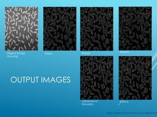
„ The function ‘edge’ is used in MATLAB for edge detection.
Slide created by Ratnamanjuri Devi, Research Assistant, MIRC

5. GRADIENT EDGE DETECTORS
These edge detectors use their respective masks shown on
the right to digitally approximate the first derivatives Gx
and Gy, using which the gradient is calculated;
g = [Gx2 + Gy2]1/2
The pixel is then said to be an edge pixel if g ≥ T, where T is
the specified threshold.
„ Sobel Edge Detector:
Syntax:
G = edge (f, ‘Sobel’, T, dir); where dir can be
‘Horizontal’, ’Vertical’ or ‘both’.
„ Prewitt Edge Detector:
Syntax:
G = edge (f,’Prewitt’, T, dir);
It is simpler to implement than Sobel but more
susceptible to noise.
„ Roberts Edge Detector:
Syntax:
G = edge (f,’Roberts’), T, dir);
Simplest and oldest edge detector. It is used to detect
edges at 45° angles. Slide created by Ratnamanjuri Devi, Research Assistant, MIRC
-1 -2 -1
0 0 0
1 2 1
-1 0 1
-2 0 2
-1 0 1
z1 z2 z3
z4 z5 z6
z7 z8 z9
-1 0 1
-1 0 1
-1 0 1
-1 -1 -1
0 0 0
1 1 1
-1 0
0 1
0 -1
1 0
Image
Neighbourhood
Sobel
Roberts
Prewitt

6. SECOND ORDER DERIVATIVE EDGE DETECTORS
„ Laplacian of Gaussian:
§ The image is first smoothened using Gaussian filter. Hence, removing
high frequency noises.
§ It then yields a Laplacian which yields a double edge image.
§ Finding the zero crossing between the two edges gives us the edge.
Syntax:
G = edge(f, ‘log’, T, sigma); where sigma is the standard deviation of
the Gaussian filter, which determines the degree of image smoothening.
„ Canny Edge Detector:
§ Most powerful edge detector provided by function ‘edge’.
§ Image is smoothened using a Gaussian filter, after which its Gradient is
calculated using either of the three detectors.
§ It uses two thresholds, one for weak edges and other for strong edges
Syntax:
G = edge(f, ‘canny’, T, sigma); where T = [T1 T2]
Slide created by Ratnamanjuri Devi, Research Assistant, MIRC

7. OUTPUT IMAGES
Original Image
‘rice.png’
PrewittSobel
Laplacian of
Gaussian
Roberts
Canny
Slide created by Ratnamanjuri Devi, Research A

8. BIBLIOGRAPHY
„ Digital Image Processing using MATLAB, Rafael
Gonzalez, Richard E. Woods and Steven L.
Eddins.
Slide created by Ratnamanjuri Devi, Research A

9. Filtered Back
Projection
A MATLAB implementation
Slide created by Ratnamanjuri Devi, Research Assistant,
MIRC

10. Joseph Hornack, Text on MRI

11. Basic Outline of the
Program
Algorithm:
• Read the image. Here, the Shepp-Logan
phantom of size 256x256.
• Generate the Sinogram of the image
assuming an incident parallel beam
rotated through 180° of the image.
• Reconstruct image from the sinogram
using filtered back projection.
• Display Original and Reconstructed
Images.
Slide created by Ratnamanjuri Devi, Research Assistant, MIRC
START
Generate
Sinogram
Reconstruct
Image from
Sinogram
END
Read
Image:
I=phantom
(256)
Display
Original and
Reconstruct
ed Images

12. Sinogram
Generation
Algorithm:
• The image is read.
• For every degree rotation of the image
starting from 0° to 179° ( a total of
180°), the sum of pixels falling along
each of the 256 lines is calculated.
• The sum of each of these rotations
result in an array of size 1x256 and
occupies the position of being the ith
column of the matrix ‘sinogram’, i-1
being the iterative rotation.
• The sinogram generated is thus a
matrix of size 256x180.
Slide created by Ratnamanjuri Devi, Research Assistant, MIRC
START
Read
Image
Input thetak
= 0° to179°
Rotate
image at
thetak
degree
sinogram(:,i+
1)= sum of
rotated
image
Display
sinogra
m
A
i=i+1
i<18
0
i=1
yes
no
Flowchart

13. Image
Reconstruction using
Filtered Back
Projection
Algorithm:
• Create a ramp filter of size
256x1 in frequency domain
• FFT of each column of the
sinogram is multiplied with
this filter and filtered
sinogram is stored in
sinogram_filt after IFFT.
• Each column of this filtered
sinogram is replicated to form
a 256x256 matrix each.
• These sinograms are rotated
back through 0,-1…-179° and
added together.
• The resulting matrix is
normalized to give the
reconstructed image.
• The images are displayed.
Slide created by Ratnamanjuri Devi, Research Assistant, MIRC
Create a ramp
filter M_filt
j=1
j<18
0
Temp1=FFT of
sinogram(:,j)*M
_filt
Sinogram_filt(:,j)=
IFFT(temp1)
j=j+1
K<180
Use repmat to
replicate
sinogram_filt(:,k)
to a 256x256
matrix
Rotate matrix by
k degrees.
phat=phat+rotat
ed matrix
k=k+1
k=1, Initialize an
empty matrix
phat(256,256)
Phat/
max(phat(:)) Display
images
END
Flowchart

14. Output Images
Slide created by Ratnamanjuri Devi, Research Assistant, MIRC
50 100 150 200 250
50
100
150
200
250
20 40 60 80 100 120 140 160 180
50
100
150
200
250
20 40 60 80 100 120 140 160 180
50
100
150
200
250
50 100 150 200 250
50
100
150
200
250
Sinogram Filtered Sinogram
Original Phantom Reconstructed Phantom

15. SENSE RECONSTRUCTION
Slides Prepared By: Shamshia Tabassum, RA, MIRC
15

16. INTRODUCTION
• SENSi-vity Encoding (SENSE) - parallel imaging technique, where an array of
mul?ple, simultaneously operated receiver coils is used for signal acquisi?on
• SENSE is based on use of mul?ple RF coils and receivers. The coil elements
are used to measure the anatomical region of interest simultaneously
• This allows reduc?on of the total scan ?me by a factor up to the number of
coil elements
• Reconstruc?on in the image domain
Reconstruc-on strategies
• strong reconstruc-on - aims at op?mizing voxel shape
• weak reconstruc-on - the voxel shape criterion is weaker in favor of the SNR
16

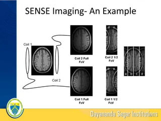
17. METHOD
Sense Reconstruc-on
1. The crea?on of an aliased, reduced FOV image for each coil array
element
2. A full FOV image is created by reversing the aliasing effect (i.e.
unfolding)
S1AA+S1BB S2AA+S2BB
S3AA+S3BB S4AA+S4BB
[y1]= [S1A S1B ]
[y2]= [S2A S2B ] [A]
[y3]= [S3A S3B ] [B]
[y4]= [S4A S4B ]
Solving Matrix -----------à
17

18. SENSE Imaging- An Example
18

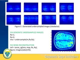
19. RESULTS
Figure 3 : Parallel acquisi?on in MRI using 8 coil array (a):cartoon depic?on (b): from matlab code(clockwise)
%% PSUEDO CODE
load('brain_8ch.mat');
[m,n,t]=size(im);
for i=1:t
imagesc(abs(im(:,:,i)));
end %% MULTICOIL RECONSTRUCTION
mul?coil_recon = abs(sum(im,3));
mul?coil_sq_recon = sqrt(abs(sum(abs(im.^2),3)));
19

20. Figure 5 : Generated undersampled images (clockwise)
20 40 60 80 100 120 140 160 180 200 220
20
40
60
80
100
120
140
160
%% SENSE RECONSTRUCTION
imf = sense_sg(ima, map, Rx, Ry);
figure; imagesc(abs(imf));
%% GENERATE UNDERSAMPLED IMAGES
Rx=1;
Ry=2;
ima = undersample(im,Rx,Ry);
20

21. REFERENCE
[1] Pruessmann KP, Weiger M, Scheidegger MB, Boesiger P,
“SENSE: Sensi?vity encoding for fast MRI”, Magne?c
Resonance in Medicine 1999; 42(5):952-962
[2] David J Larkman, Rita G Nunes, “Parallel magne?c
resonance imaging”, Phys. Med. Biol. 52 (2007) R15–
R55
[3] “Role of Parallel Imaging in Magne?c Resonance
Imaging”,Douglas C. Noll & Bradley P. Suqon,
Department of Biomedical Engineering, University of
Michigan Field Func?onal MRI
21

22. Acknowledgements/Contact info
• MIRC members, Medical Electronics members
• Management, DSI
• Academic and Industrial partners
• MIRC_HOME_OFFLINE (hqp://www.dayanandasagar.edu/mirc-home.html)
• MIRC_SHARING_OFFLINE
• MIRC_PEOPLE_OFFLINE
• sairam.geethanath@dayanandasagar.edu
22

23. X
2D
IFFT
10
20
30
40
50
60
70
10
20
30
40
50
60
70
Uniform
Sampling
X
2D
IFFT
20
40
60
80
100
120
20
40
60
80
100
120
Incoherent
Sampling