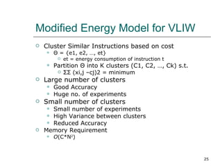
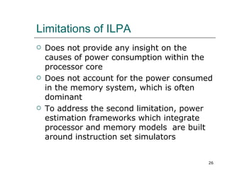
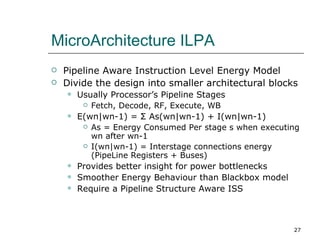
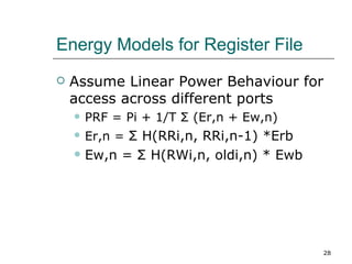
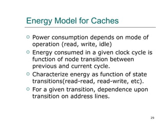
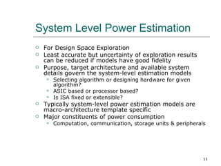
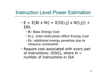
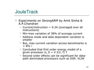
Instruction Level Power Analysis


                                   1
Layout
   Introduction
   Components of Power Consumption
   Power Characterization
   Instruction Level Power Analysis for RISC
    processors
   Extensions for VLIW/EPIC processors
   Register Files
   Caches


                                                2
Introduction
   Why power of nano-electronics became so
    important?
       Because of Moore’s law still holds true through
        complex applications
       Mobile systems – battery “bottleneck”
       High performance computation – heat
        extraction
       Operating cost and reliability
          Data warehouse of ISP with 8000 servers

           needs 2 MW


                                                          3
Introduction
   Power or Energy? Aren’t they go hand-in-hand?
       Power varies significantly with time!
       A given battery has fixed amount of energy
       Average power consumption = Energy/Execution-
        time
            Decides average chip and junction temperature
            Decides battery life (if peak current < rated
             current)
       Peak power and current
            Voltage drops, hot spots, rate of battery discharge
   Power-efficient, Energy-efficient, Battery-efficient
    design paradigms do exist!


                                                                   4
Components of Power
Consumption
   System = hardware platform + software (sys. & app.)
       Software impacts hardware power consumption
   Static power
       Sub-threshold leakage & reverse biased junction leakage
       Quiescent biasing power (in case of non-CMOS circuits)
   Dynamic power
       Charging and discharging of capacitance (switching
        activity)
       Short circuit power during transition (rate of change,
        delay)
       Alternative grouping (used at component/cell level)
            Switching power at the boundaries of cells
            Internal cell power
                  Short circuit power
                  Switching power at internal nodes


                                                                  5
System Abstractions - Power
                                  Functional Specifications and Constraints


                                                                              Accuracy of power characterization
Opportunities for optimization


                                            System Level Netlist


                                                                                                                   Time complexity
                                    Register Transfer Level (RTL) Netlist

                                        Component/Cell Level Netlist

                                        Layout or Configuration-bits

                                                    Chip


                                                                                                                          6
Power Characterization
   Measurement (Chip/Board Level)
       Most accurate
       Perhaps the fastest, if setup and tools
        exist
       Too late to change hardware details
       Software/Load control is still possible
       Typically used for software
        optimizations


                                              7
Power Characterization (cont…)
   Transistor Level (estimation)
       Spice simulation of transistor level netlist
       Most accurate in the simulation world
       Requires complete implementation details
       Unmanageable time complexity even for
        simpler designs
       Typically used for cell/component
        characterization
       Synopsys PowerMill (said to provide spice-
        like accuracy)


                                                       8
Power Characterization (cont…)
   Cell Level (estimation)
       After logic synthesis
       Requires RTL implementation
       Simulation to capture switching activity
            Requires delay simulation if glitches need to be accounted
       Characterized cells – empirical formulas or table look-up
       Interconnect power
            Either unaccounted or
            Using estimated wire load models (typically based on
             experience) or
            Extracted layout (if done after physical synthesis)
       Still unmanageable time complexity especially to use in
        design space exploration
       Synopsys PrimePower
            Netlist, interconnect capacitance, VCD traces, cell power
             library


                                                                          9
Power Characterization (cont…)
   Register Transfer Level (estimation)
       Requires conceptual RTL description (detailed
        micro-architecture)
       Data-path is modeled as netlist of macro cells,
        which are characterized offline
       Control path and glue logic
            Either unaccounted or estimated based on I/O
       Simulation to capture switching activity
            Typically glitches are not considered but methods do
             exist
       Interconnect power
            Typically unaccounted but possible to estimate
             through floor-planning
       Typically used in DSE mostly using in-house tools


                                                                    10
System Level Power Estimation
   For Design Space Exploration
   Least accurate but uncertainty of exploration results
    can be reduced if models have good fidelity
   Purpose, target architecture and available system
    details govern the system-level estimation models
       Selecting algorithm or designing hardware for given
        algorithm?
       ASIC based or processor based?
       Is ISA fixed or extensible?
   Typically system-level power estimation models are
    macro-architecture template specific
   Major constituents of power consumption
       Computation, communication, storage units & peripherals


                                                              11
Power Estimation Models
   Activity Based Models
   Instruction Level Energy Models


                                      12
Activity Based Models
   Fixed Activity Model
   N-Transition Model
   Dual Bit Model


                           13
Fixed Activity Model

                   P = ∑ i kiGifi
Where:
ki = PFA proportionality constant extracted
   empirically from past designs
Gi = Measure of hardware complexity
fi = Activation frequency

   Disadvantage: Do not model the influence of data
    activity on power consumption


                                                   14
N-Transition Model

               P = Pconst + n.Pchange

   Disadvantage:
    It does not differentiate between transitions on
     different inputs.


                                                       15
Dual Bit Type Model
   Drawback in previous
    approaches:
       Less Accurate
       Characterizes the
        module on basis of
        Uniform White Noise
        (UWN) input
       Leads to high error if
        the input dynamic
        range does not fully
        occupy the word
        length


                                 16
Dual Bit Type Model
The Approach

   Combines reduced complexity of the
    architecture level with the accuracy of
    gate and circuit level
   Black box model of capacitance switched
    in each module for various types of inputs
   Easy to parameterize capacitance models
    to take into account size , etc.


                                             17
Dual Bit Type Model
Modeling Complexity
   Power consumed by a module is a
    function of its complexity as large
    modules contain more circuitry
   Examples:
       Capacitance of N-bit ripple carry subtracter:
               CT = Ceff * N
       Not restricted to linear models, but can be
        used to specify even more complex models


                                                        18
Dual Bit Type Model
Capacitive Data Coefficients

   Describe the average amount of
    capacitance switched within a module
    during an input transition
       LSB regions suffer random transitions and
        hence can be characterized by a single
        capacitive coefficient CUU
       MSB region experiences sign transitions and so
        is characterized by capacitive sign coefficients
        C+-,C++, etc.


                                                      19
Instruction Level Power Estimation
     First introduced to characterize
      processor power consumption to drive
      software optimizations
     Each instruction is associated with
      some current
     Inter instruction effects for better
      accuracy


                                         20
Instruction Level Power Estimation
     E = Σ(Bi x Ni) + Σ(O(i,j) x N(I,j)) +
      ΣEk
        Bi: Base Energy Cost
        Oi.j: Inter-instruction effect Energy Cost

        Ek: additional energy penalties due to

         resource constraints
     Require cost associated with every pair
      of instructions: O(N2), where N =
      number of instructions in ISA


                                                      21
JouleTrack
   Experiments on StrongARM by Amit Sinha &
    A.P.Chandran
       Current/instruction ~ 0.2A (averaged over all
        instructions)
       Min-max variation of 38% of average current
       Address mode and data dependent variation is
        smaller
       But, max current variation across benchmarks is
        < 8% !
       Concluded that first order energy model of a
        given processor is, E = V I(V, f) T
       Second order effects can be significant for data-
        path dominated processors such as DSP, VLIW


                                                        22
Instruction Level Power Estimation
   Impractical for CISC processors with
    very large instruction set
       Higher Average Instruction Energy
       Low Energy Per Instruction Variance
       Do not consider inter instruction effects
       Cluster Similar Instructions as a single
        class
   Exponential Storage Problem for VLIW
    architectures
       No. of Long Instructions = N operations
        into a K-wide VLIW = N(2k)


                                                    23
Modified Energy Model for VLIW
   Assume Independent Energy dissipation for
    different Execution slots
   Consider nop as the base energy
      E(W) = ΣU(wn|wn-1) + mxpxS + lxqxM

      U(wn|wn-1) = U(0|0) + Σv(wnk,wn-1k)

            Wnk = operation issued on lane k by instruction wn
       Example
            Wn = [ ALU NOP NOP NOP], Wn-1 = [ LS NOP ALU
             NOP]
            U(wn|wn-1) = U(0|0) + v(ALU|LS) + v(NOP|ALU)
   Memory Requirement
       O(K*N2)

                                                             24
Modified Energy Model for VLIW
   Cluster Similar Instructions based on cost
       Θ = {e1, e2, …, et}
            et = energy consumption of instruction t
       Partition Θ into K clusters (C1, C2, …, Ck) s.t.
            ΣΣ (xi,j –cj)2 = minimum
   Large number of clusters
       Good Accuracy
       Huge no. of experiments
   Small number of clusters
      Small number of experiments
      High Variance between clusters
      Reduced Accuracy
   Memory Requirement
       O(C*N2)


                                                           25
Limitations of ILPA
   Does not provide any insight on the
    causes of power consumption within the
    processor core
   Does not account for the power consumed
    in the memory system, which is often
    dominant
   To address the second limitation, power
    estimation frameworks which integrate
    processor and memory models are built
    around instruction set simulators


                                          26
MicroArchitecture ILPA
   Pipeline Aware Instruction Level Energy Model
   Divide the design into smaller architectural blocks
       Usually Processor’s Pipeline Stages
            Fetch, Decode, RF, Execute, WB
       E(wn|wn-1) = Σ As(wn|wn-1) + I(wn|wn-1)
            As = Energy Consumed Per stage s when executing
             wn after wn-1
            I(wn|wn-1) = Interstage connections energy
             (PipeLine Registers + Buses)
       Provides better insight for power bottlenecks
       Smoother Energy Behaviour than Blackbox model
       Require a Pipeline Structure Aware ISS


                                                          27
Energy Models for Register File
   Assume Linear Power Behaviour for
    access across different ports
       PRF = Pi + 1/T Σ (Er,n + Ew,n)
       Er,n = Σ H(RRi,n, RRi,n-1) *Erb
       Ew,n = Σ H(RWi,n, oldi,n) * Ewb


                                          28
Energy Model for Caches
   Power consumption depends on mode of
    operation (read, write, idle)
   Energy consumed in a given clock cycle is
    function of node transition between
    previous and current cycle.
   Characterize energy as function of state
    transitions(read-read, read-write, etc).
   For a given transition, dependence upon
    transition on address lines.


                                            29
Thank You


            30

Instruction level power analysis

  • 1.
  • 2.
    Layout  Introduction  Components of Power Consumption  Power Characterization  Instruction Level Power Analysis for RISC processors  Extensions for VLIW/EPIC processors  Register Files  Caches 2
  • 3.
    Introduction  Why power of nano-electronics became so important?  Because of Moore’s law still holds true through complex applications  Mobile systems – battery “bottleneck”  High performance computation – heat extraction  Operating cost and reliability  Data warehouse of ISP with 8000 servers needs 2 MW 3
  • 4.
    Introduction  Power or Energy? Aren’t they go hand-in-hand?  Power varies significantly with time!  A given battery has fixed amount of energy  Average power consumption = Energy/Execution- time  Decides average chip and junction temperature  Decides battery life (if peak current < rated current)  Peak power and current  Voltage drops, hot spots, rate of battery discharge  Power-efficient, Energy-efficient, Battery-efficient design paradigms do exist! 4
  • 5.
    Components of Power Consumption  System = hardware platform + software (sys. & app.)  Software impacts hardware power consumption  Static power  Sub-threshold leakage & reverse biased junction leakage  Quiescent biasing power (in case of non-CMOS circuits)  Dynamic power  Charging and discharging of capacitance (switching activity)  Short circuit power during transition (rate of change, delay)  Alternative grouping (used at component/cell level)  Switching power at the boundaries of cells  Internal cell power  Short circuit power  Switching power at internal nodes 5
  • 6.
    System Abstractions -Power Functional Specifications and Constraints Accuracy of power characterization Opportunities for optimization System Level Netlist Time complexity Register Transfer Level (RTL) Netlist Component/Cell Level Netlist Layout or Configuration-bits Chip 6
  • 7.
    Power Characterization  Measurement (Chip/Board Level)  Most accurate  Perhaps the fastest, if setup and tools exist  Too late to change hardware details  Software/Load control is still possible  Typically used for software optimizations 7
  • 8.
    Power Characterization (cont…)  Transistor Level (estimation)  Spice simulation of transistor level netlist  Most accurate in the simulation world  Requires complete implementation details  Unmanageable time complexity even for simpler designs  Typically used for cell/component characterization  Synopsys PowerMill (said to provide spice- like accuracy) 8
  • 9.
    Power Characterization (cont…)  Cell Level (estimation)  After logic synthesis  Requires RTL implementation  Simulation to capture switching activity  Requires delay simulation if glitches need to be accounted  Characterized cells – empirical formulas or table look-up  Interconnect power  Either unaccounted or  Using estimated wire load models (typically based on experience) or  Extracted layout (if done after physical synthesis)  Still unmanageable time complexity especially to use in design space exploration  Synopsys PrimePower  Netlist, interconnect capacitance, VCD traces, cell power library 9
  • 10.
    Power Characterization (cont…)  Register Transfer Level (estimation)  Requires conceptual RTL description (detailed micro-architecture)  Data-path is modeled as netlist of macro cells, which are characterized offline  Control path and glue logic  Either unaccounted or estimated based on I/O  Simulation to capture switching activity  Typically glitches are not considered but methods do exist  Interconnect power  Typically unaccounted but possible to estimate through floor-planning  Typically used in DSE mostly using in-house tools 10
  • 11.
    System Level PowerEstimation  For Design Space Exploration  Least accurate but uncertainty of exploration results can be reduced if models have good fidelity  Purpose, target architecture and available system details govern the system-level estimation models  Selecting algorithm or designing hardware for given algorithm?  ASIC based or processor based?  Is ISA fixed or extensible?  Typically system-level power estimation models are macro-architecture template specific  Major constituents of power consumption  Computation, communication, storage units & peripherals 11
  • 12.
    Power Estimation Models  Activity Based Models  Instruction Level Energy Models 12
  • 13.
    Activity Based Models  Fixed Activity Model  N-Transition Model  Dual Bit Model 13
  • 14.
    Fixed Activity Model P = ∑ i kiGifi Where: ki = PFA proportionality constant extracted empirically from past designs Gi = Measure of hardware complexity fi = Activation frequency  Disadvantage: Do not model the influence of data activity on power consumption 14
  • 15.
    N-Transition Model P = Pconst + n.Pchange  Disadvantage: It does not differentiate between transitions on different inputs. 15
  • 16.
    Dual Bit TypeModel  Drawback in previous approaches:  Less Accurate  Characterizes the module on basis of Uniform White Noise (UWN) input  Leads to high error if the input dynamic range does not fully occupy the word length 16
  • 17.
    Dual Bit TypeModel The Approach  Combines reduced complexity of the architecture level with the accuracy of gate and circuit level  Black box model of capacitance switched in each module for various types of inputs  Easy to parameterize capacitance models to take into account size , etc. 17
  • 18.
    Dual Bit TypeModel Modeling Complexity  Power consumed by a module is a function of its complexity as large modules contain more circuitry  Examples:  Capacitance of N-bit ripple carry subtracter: CT = Ceff * N  Not restricted to linear models, but can be used to specify even more complex models 18
  • 19.
    Dual Bit TypeModel Capacitive Data Coefficients  Describe the average amount of capacitance switched within a module during an input transition  LSB regions suffer random transitions and hence can be characterized by a single capacitive coefficient CUU  MSB region experiences sign transitions and so is characterized by capacitive sign coefficients C+-,C++, etc. 19
  • 20.
    Instruction Level PowerEstimation  First introduced to characterize processor power consumption to drive software optimizations  Each instruction is associated with some current  Inter instruction effects for better accuracy 20
  • 21.
    Instruction Level PowerEstimation  E = Σ(Bi x Ni) + Σ(O(i,j) x N(I,j)) + ΣEk  Bi: Base Energy Cost  Oi.j: Inter-instruction effect Energy Cost  Ek: additional energy penalties due to resource constraints  Require cost associated with every pair of instructions: O(N2), where N = number of instructions in ISA 21
  • 22.
    JouleTrack  Experiments on StrongARM by Amit Sinha & A.P.Chandran  Current/instruction ~ 0.2A (averaged over all instructions)  Min-max variation of 38% of average current  Address mode and data dependent variation is smaller  But, max current variation across benchmarks is < 8% !  Concluded that first order energy model of a given processor is, E = V I(V, f) T  Second order effects can be significant for data- path dominated processors such as DSP, VLIW 22
  • 23.
    Instruction Level PowerEstimation  Impractical for CISC processors with very large instruction set  Higher Average Instruction Energy  Low Energy Per Instruction Variance  Do not consider inter instruction effects  Cluster Similar Instructions as a single class  Exponential Storage Problem for VLIW architectures  No. of Long Instructions = N operations into a K-wide VLIW = N(2k) 23
  • 24.
    Modified Energy Modelfor VLIW  Assume Independent Energy dissipation for different Execution slots  Consider nop as the base energy  E(W) = ΣU(wn|wn-1) + mxpxS + lxqxM  U(wn|wn-1) = U(0|0) + Σv(wnk,wn-1k)  Wnk = operation issued on lane k by instruction wn  Example  Wn = [ ALU NOP NOP NOP], Wn-1 = [ LS NOP ALU NOP]  U(wn|wn-1) = U(0|0) + v(ALU|LS) + v(NOP|ALU)  Memory Requirement  O(K*N2) 24
  • 25.
    Modified Energy Modelfor VLIW  Cluster Similar Instructions based on cost  Θ = {e1, e2, …, et}  et = energy consumption of instruction t  Partition Θ into K clusters (C1, C2, …, Ck) s.t.  ΣΣ (xi,j –cj)2 = minimum  Large number of clusters  Good Accuracy  Huge no. of experiments  Small number of clusters  Small number of experiments  High Variance between clusters  Reduced Accuracy  Memory Requirement  O(C*N2) 25
  • 26.
    Limitations of ILPA  Does not provide any insight on the causes of power consumption within the processor core  Does not account for the power consumed in the memory system, which is often dominant  To address the second limitation, power estimation frameworks which integrate processor and memory models are built around instruction set simulators 26
  • 27.
    MicroArchitecture ILPA  Pipeline Aware Instruction Level Energy Model  Divide the design into smaller architectural blocks  Usually Processor’s Pipeline Stages  Fetch, Decode, RF, Execute, WB  E(wn|wn-1) = Σ As(wn|wn-1) + I(wn|wn-1)  As = Energy Consumed Per stage s when executing wn after wn-1  I(wn|wn-1) = Interstage connections energy (PipeLine Registers + Buses)  Provides better insight for power bottlenecks  Smoother Energy Behaviour than Blackbox model  Require a Pipeline Structure Aware ISS 27
  • 28.
    Energy Models forRegister File  Assume Linear Power Behaviour for access across different ports  PRF = Pi + 1/T Σ (Er,n + Ew,n)  Er,n = Σ H(RRi,n, RRi,n-1) *Erb  Ew,n = Σ H(RWi,n, oldi,n) * Ewb 28
  • 29.
    Energy Model forCaches  Power consumption depends on mode of operation (read, write, idle)  Energy consumed in a given clock cycle is function of node transition between previous and current cycle.  Characterize energy as function of state transitions(read-read, read-write, etc).  For a given transition, dependence upon transition on address lines. 29
  • 30.