Downloaded 104 times
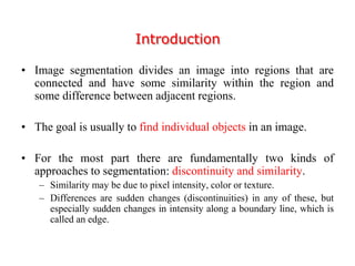
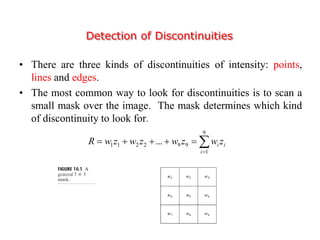
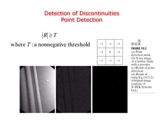
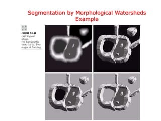
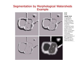
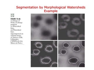
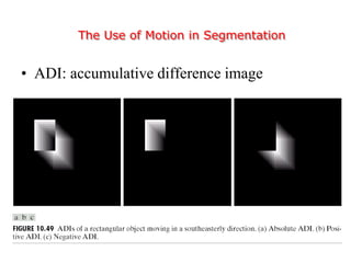
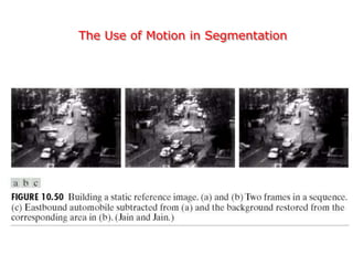

This document discusses various techniques for image segmentation. It describes two main approaches to segmentation: discontinuity-based methods that detect edges or boundaries, and region-based methods that partition an image into uniform regions. Specific techniques discussed include thresholding, gradient operators, edge detection, the Hough transform, region growing, region splitting and merging, and morphological watershed transforms. Motion can also be used for segmentation by analyzing differences between frames in a video.