image process

1. Image Enhancement
(Point Processing)
Syed Ali Zamin
1

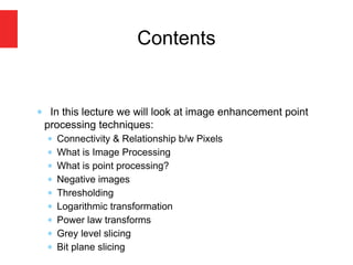
2.  In this lecture we will look at image enhancement point
processing techniques:
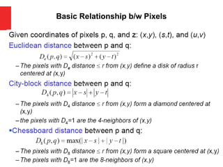
 Connectivity & Relationship b/w Pixels
 What is Image Processing
 What is point processing?
 Negative images
 Thresholding
 Logarithmic transformation
 Power law transforms
 Grey level slicing
 Bit plane slicing
Contents

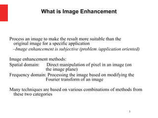
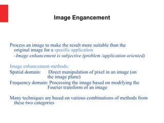
3. Process an image to make the result more suitable than the
original image for a specific application
–Image enhancement is subjective (problem /application oriented)
Image enhancement methods:
Spatial domain: Direct manipulation of pixel in an image (on
the image plane)
Frequency domain: Processing the image based on modifying the
Fourier transform of an image
Many techniques are based on various combinations of methods from
these two categories
3
What is Image Enhancement

4. Relationship Between Pixels

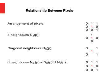
5.  Establishing boundaries of objects and components of
regions in an image.
 Group the same region by assumption that the pixels
being the same color or equal intensity will have the
same region
 Two pixels may be four neighbors, but they are said
to be connected only if they have the same value
(gray level)
Connectivity

6. 6
Basic Relationship b/w Pixels

7. 7
Basic Relationship b/w Pixels

8. 8
Basic Relationship b/w Pixels

9. 9
Basic Relationship b/w Pixels

10. So far when we have spoken about image grey level
values we have said they are in the range [0, 255]
 Where 0 is black and 255 is white
There is no reason why we have to use this range
 The range [0,255] stems from display technologes
For many of the image processing operations in this
lecture grey levels are assumed to be given in the range
[0.0, 1.0]
A Note About Grey Levels

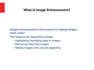
11. Image enhancement is the process of making images
more useful
The reasons for doing this include:
 Highlighting interesting detail in images
 Removing noise from images
 Making images more visually appealing
What Is Image Enhancement?

12. Image Enhancement Examples

13. Image Enhancement Examples (cont…)

14. Image Enhancement Examples (cont…)

15. Image Enhancement Examples (cont…)

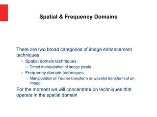
16. There are two broad categories of image enhancement
techniques
 Spatial domain techniques
 Direct manipulation of image pixels
 Frequency domain techniques
 Manipulation of Fourier transform or wavelet transform of an
image
For the moment we will concentrate on techniques that
operate in the spatial domain
Spatial & Frequency Domains

17. Process an image to make the result more suitable than the
original image for a specific application
–Image enhancement is subjective (problem /application oriented)
Image enhancement methods:
Spatial domain: Direct manipulation of pixel in an image (on
the image plane)
Frequency domain: Processing the image based on modifying the
Fourier transform of an image
Many techniques are based on various combinations of methods from
these two categories
Image Engancement

18. 18
Image Enhancement

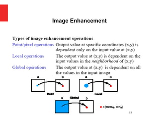
19. Spatial domain enhancement methods can be generalized as
g(x,y)=T[f(x,y)]
f(x,y): input image
g(x,y): processed (output) image
T[*]: an operator on f (or a set of input images),
defined over neighborhood of (x,y)
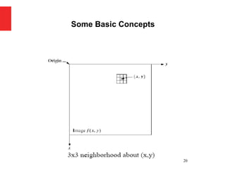
Neighborhood about (x,y): a square or rectangular
sub-image area centered at (x,y)
19
Some Basic Concepts

20. 20
Some Basic Concepts

21. g(x,y) = T [f(x,y)]
Pixel/point operation:
Neighborhood of size 1x1: g depends only on f at (x,y)
T: a gray-level/intensity transformation/mapping function
Let r = f(x,y) s = g(x,y)
r and s represent gray levels of f and g at (x,y)
Then s = T(r)
Local operations:
g depends on the predefined number of neighbors of f at (x,y)
Implemented by using mask processing or filtering
Masks (filters, windows, kernels, templates) :
a small (e.g. 3×3) 2-D array, in which the values of the
coefficients determine the nature of the process
Some Basic Concepts

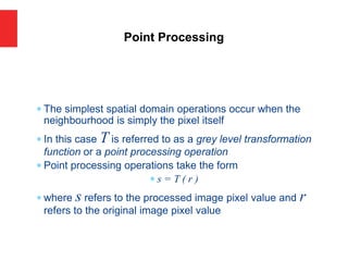
22.  The simplest spatial domain operations occur when the
neighbourhood is simply the pixel itself
 In this case T is referred to as a grey level transformation
function or a point processing operation
 Point processing operations take the form
 s = T ( r )
 where s refers to the processed image pixel value and r
refers to the original image pixel value
Point Processing

23. 23
▪ Image Negatives
▪ Log Transformations
▪ Power-Law Transformations
Common Pixel Operations

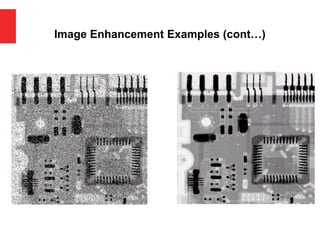
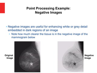
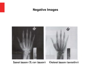
24.  Negative images are useful for enhancing white or grey detail
embedded in dark regions of an image
 Note how much clearer the tissue is in the negative image of the
mammogram below
Point Processing Example:
Negative Images
Original
Image
Negative
Image

25. Negative Images

26. Point Processing Example:
Negative Images (cont…)
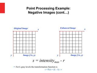
Original Image x
y Image f (x, y)
Enhanced Image x
y Image f (x, y)
s = intensitymax - r
▪ For L gray levels the transformation function is
s =T(r) = (L - 1) - r

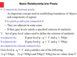
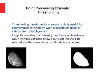
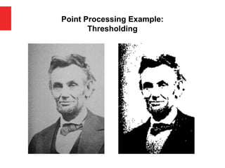
27.  Thresholding transformations are particularly useful for
segmentation in which we want to isolate an object of
interest from a background
 Image Thresholding is an intensity transformation function in
which the values of pixels below a particular threshold are
reduced, and the values above that threshold are boosted
Point Processing Example:
Thresholding
s =
255
0 r <= threshold
r > threshold

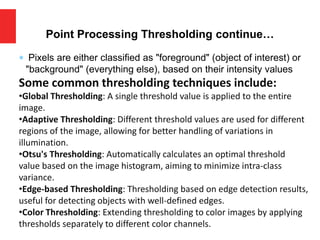
28.  Pixels are either classified as "foreground" (object of interest) or
"background" (everything else), based on their intensity values
Some common thresholding techniques include:
•Global Thresholding: A single threshold value is applied to the entire
image.
•Adaptive Thresholding: Different threshold values are used for different
regions of the image, allowing for better handling of variations in
illumination.
•Otsu's Thresholding: Automatically calculates an optimal threshold
value based on the image histogram, aiming to minimize intra-class
variance.
•Edge-based Thresholding: Thresholding based on edge detection results,
useful for detecting objects with well-defined edges.
•Color Thresholding: Extending thresholding to color images by applying
thresholds separately to different color channels.
Point Processing Thresholding continue…

29. Point Processing Example:
Thresholding

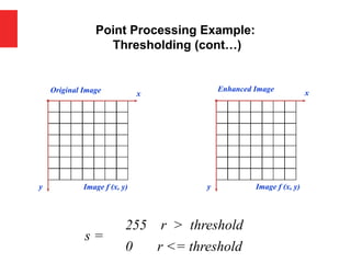
30. Point Processing Example:
Thresholding (cont…)
Original Image x
y Image f (x, y)
Enhanced Image x
y Image f (x, y)
s =
0 r <= threshold
255 r > threshold

31. Intensity Transformations

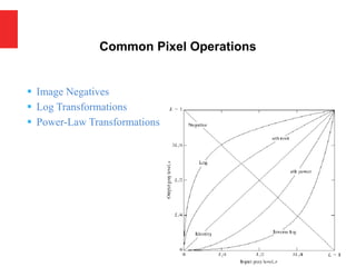
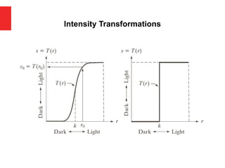
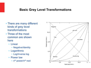
32.  There are many different
kinds of grey level
transformations
 Three of the most
common are shown
here
 Linear
 Negative/Identity
 Logarithmic
 Log/Inverse log
 Power law
 nth power/nth root
Basic Grey Level Transformations

33. s =T(r) = a.r (a is a constant)
Image Scaling

34. Image Scaling

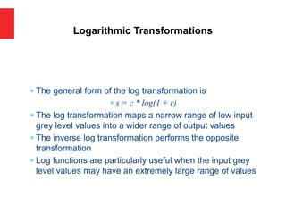
35.  The general form of the log transformation is
 s = c * log(1 + r)
 The log transformation maps a narrow range of low input
grey level values into a wider range of output values
 The inverse log transformation performs the opposite
transformation
 Log functions are particularly useful when the input grey
level values may have an extremely large range of values
Logarithmic Transformations

36. Logarithmic Transformations (cont…)

37. 08/01/2018
37
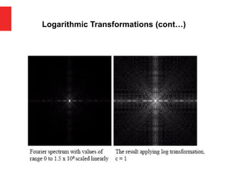
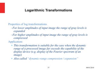
Properties of log transformations
–For lower amplitudes of input image the range of gray levels is
expanded
–For higher amplitudes of input image the range of gray levels is
compressed
Application:
 This transformation is suitable for the case when the dynamic
range of a processed image far exceeds the capability of the
display device (e.g. display of the Fourier spectrum of an
image)
 Also called “dynamic-range compression / expansion”
Logarithmic Transformations

38. Logarithmic Transformations (cont…)
Original Image x
y Image f (x, y)
Enhanced Image x
y Image f (x, y)
s = log(1 + r)
We usually set c to 1
Grey levels must be in the range [0.0, 1.0]

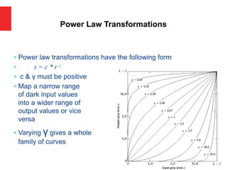
39.  Power law transformations have the following form
 s = c * r γ
 c & γ must be positive
 Map a narrow range
of dark input values
into a wider range of
output values or vice
versa
 Varying γ gives a whole
family of curves
Power Law Transformations

40.  We usually set c to 1
 Grey levels must be in the range [0.0, 1.0]
Power Law Transformations (cont…)
Original Image x
y Image f (x, y)
Enhanced Image x
y Image f (x, y)
s = r γ

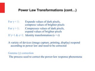
41. For γ < 1: Expands values of dark pixels,
compress values of brighter pixels
For γ > 1: Compresses values of dark pixels,
expand values of brighter pixels
If γ=1 & c=1: Identity transformation (s = r)
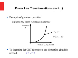
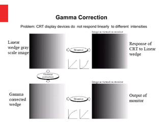
A variety of devices (image capture, printing, display) respond
according to power law and need to be corrected
Gamma (γ) correction
The process used to correct the power-law response phenomena
Power Law Transformations (cont…)

42. Power Law Example

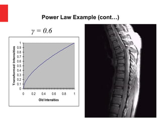
43. Power Law Example (cont…)
γ = 0.6
0
0.1
0.2
0.3
0.4
0.5
0.6
0.7
0.8
0.9
1
0 0.2 0.4 0.6 0.8 1
Old Intensities
Transformed
Intensities

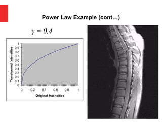
44. Power Law Example (cont…)
γ = 0.4
0
0.1
0.2
0.3
0.4
0.5
0.6
0.7
0.8
0.9
1
0 0.2 0.4 0.6 0.8 1
Original Intensities
Transformed
Intensities

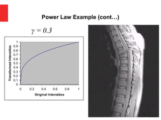
45. Power Law Example (cont…)
γ = 0.3
0
0.1
0.2
0.3
0.4
0.5
0.6
0.7
0.8
0.9
1
0 0.2 0.4 0.6 0.8 1
Original Intensities
Transformed
Intensities

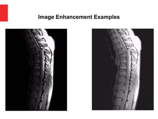
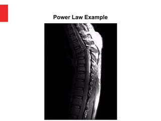
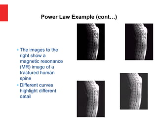
46.  The images to the
right show a
magnetic resonance
(MR) image of a
fractured human
spine
 Different curves
highlight different
detail
Power Law Example (cont…)

47. Power Law Example
γ = 1.0

48. Power Law Example (cont…)
γ = 3.0

49. Power Law Example (cont…)
γ = 4.0

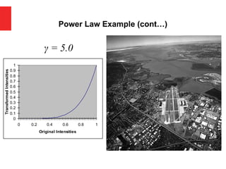
50. Power Law Example (cont…)
γ = 5.0
0
0.1
0.2
0.3
0.4
0.5
0.6
0.7
0.8
0.9
1
0 0.2 0.4 0.6 0.8 1
Original Intensities
Transformed
Intensities

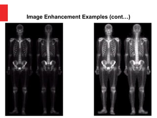
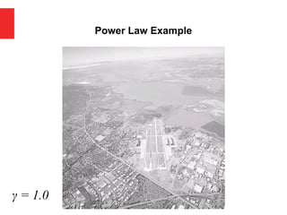
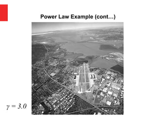
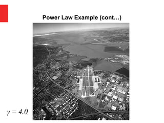
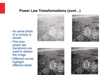
51.  An aerial photo
of a runway is
shown
 This time
power law
transforms are
used to darken
the image
 Different curves
highlight
different detail
Power Law Transformations (cont…)

52. 52
Power Law Transformations (cont…)

53. Gamma Correction
Problem: CRT display devices do not respond linearly to different intensities

54. More Contrast Issues

55. More Contrast Issues

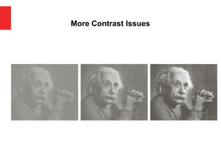
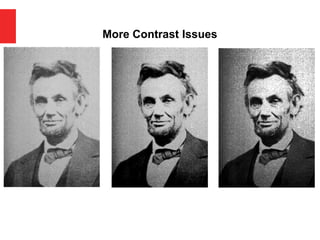
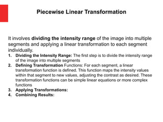
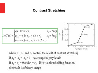
56. Piecewise Linear Transformation
It involves dividing the intensity range of the image into multiple
segments and applying a linear transformation to each segment
individually.
1. Dividing the Intensity Range: The first step is to divide the intensity range
of the image into multiple segments
2. Defining Transformation Functions: For each segment, a linear
transformation function is defined. This function maps the intensity values
within that segment to new values, adjusting the contrast as desired. These
transformation functions can be simple linear equations or more complex
functions
3. Applying Transformations:
4. Combining Results:

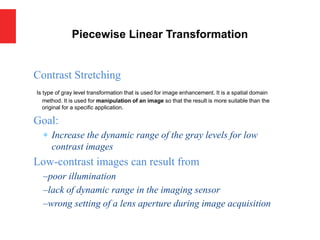
57. Piecewise Linear Transformation
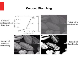
Contrast Stretching
Is type of gray level transformation that is used for image enhancement. It is a spatial domain
method. It is used for manipulation of an image so that the result is more suitable than the
original for a specific application.
Goal:
 Increase the dynamic range of the gray levels for low
contrast images
Low-contrast images can result from
–poor illumination
–lack of dynamic range in the imaging sensor
–wrong setting of a lens aperture during image acquisition

58. Contrast Stretching [continue…]
Contrast stretching, also known as histogram stretching or
normalization, is a basic image enhancement technique used to
improve the contrast in an image by expanding the range of
intensity values. The goal of contrast stretching is to utilize the
entire dynamic range of pixel values available in the image,
thereby increasing the visual separation between different
objects or features in the image.
The process of contrast stretching involves mapping the original
intensity values of the image to a new range of values. This is
typically done by linearly scaling the intensity values from their
original range to a new range, often spanning from 0 to 255 (for an
8-bit grayscale image).

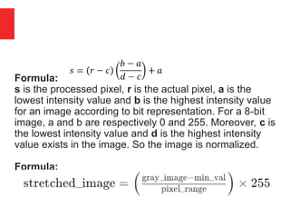
59. Formula:
s is the processed pixel, r is the actual pixel, a is the
lowest intensity value and b is the highest intensity value
for an image according to bit representation. For a 8-bit
image, a and b are respectively 0 and 255. Moreover, c is
the lowest intensity value and d is the highest intensity
value exists in the image. So the image is normalized.
Formula:

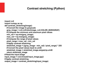
60. Contrast stretching (Python)
import cv2
import numpy as np
def contrast_stretching(image):
# Convert the image to grayscale
gray_image = cv2.cvtColor(image, cv2.COLOR_BGR2GRAY)
# Compute the minimum and maximum pixel values
min_val = np.min(gray_image)
max_val = np.max(gray_image)
# Compute the range of pixel values
pixel_range = max_val - min_val
# Apply contrast stretching
stretched_image = ((gray_image - min_val) / pixel_range) * 255
# Convert the pixel values back to uint8
stretched_image = stretched_image.astype(np.uint8
return stretched_image
# Read the input image
input_image = cv2.imread('input_image.jpg')
# Apply contrast stretching
output_image = contrast_stretching(input_image)

61. Contrast Stretching

62. 62
Contrast Stretching

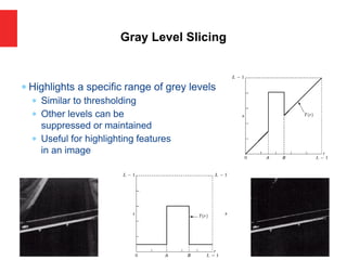
63.  Highlights a specific range of grey levels
 Similar to thresholding
 Other levels can be
suppressed or maintained
 Useful for highlighting features
in an image
Gray Level Slicing

64. Gray level slicing, also known as intensity level slicing or gray
value slicing, is an image processing technique used to
highlight specific intensity ranges within a grayscale image
while suppressing the rest. It involves selectively enhancing
or suppressing certain gray levels to emphasize particular
features or regions of interest in the image.

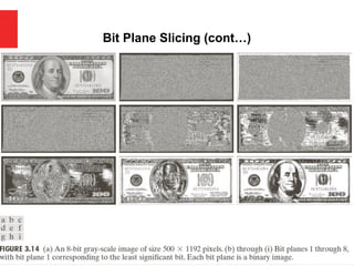
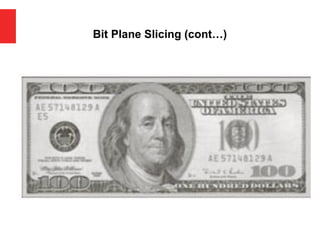
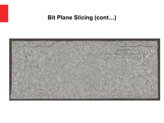
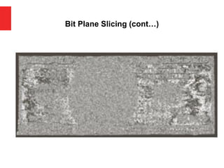
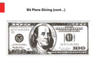
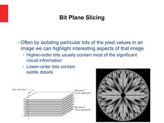
65.  Often by isolating particular bits of the pixel values in an
image we can highlight interesting aspects of that image
 Higher-order bits usually contain most of the significant
visual information
 Lower-order bits contain
subtle details
Bit Plane Slicing

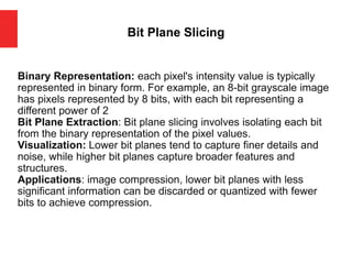
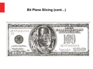
66. Bit Plane Slicing
Binary Representation: each pixel's intensity value is typically
represented in binary form. For example, an 8-bit grayscale image
has pixels represented by 8 bits, with each bit representing a
different power of 2
Bit Plane Extraction: Bit plane slicing involves isolating each bit
from the binary representation of the pixel values.
Visualization: Lower bit planes tend to capture finer details and
noise, while higher bit planes capture broader features and
structures.
Applications: image compression, lower bit planes with less
significant information can be discarded or quantized with fewer
bits to achieve compression.

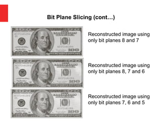
67. Bit Plane Slicing (cont…)
[10000000] [01000000]
[00100000] [00001000]
[00000100] [00000001]

68. Bit Plane Slicing (cont…)

69. Bit Plane Slicing (cont…)

70. Bit Plane Slicing (cont…)

71. Bit Plane Slicing (cont…)

72. Bit Plane Slicing (cont…)

73. Bit Plane Slicing (cont…)

74. Bit Plane Slicing (cont…)

75. Bit Plane Slicing (cont…)

76. Bit Plane Slicing (cont…)

77. Bit Plane Slicing (cont…)

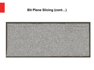
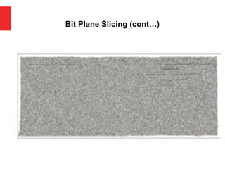
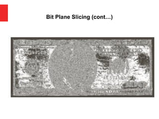
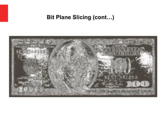
78. Bit Plane Slicing (cont…)
Reconstructed image using
only bit planes 8 and 7
Reconstructed image using
only bit planes 8, 7 and 6
Reconstructed image using
only bit planes 7, 6 and 5

79. A Different Problem

80. Lets Double the Size

81. Interpolation
Nearest Neighbor

82. What Happens When Tripling

83. Is There a Better Method
Interpolation: Bi-Linear

84. Is There be a Better Method

85. What Happens in 2D

86. Which is Better

87. Which is Better
Before Interpolation
Nearest Neighbor Bi-Linear
Original

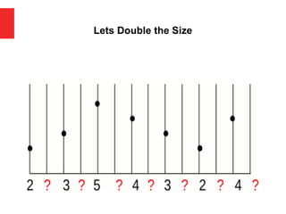
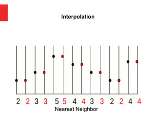
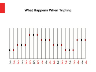
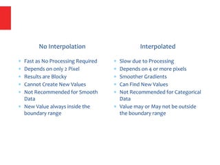
88. No Interpolation
 Fast as No Processing Required
 Depends on only 2 Pixel
 Results are Blocky
 Cannot Create New Values
 Not Recommended for Smooth
Data
 New Value always inside the
boundary range
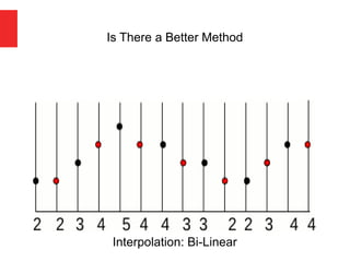
Interpolated
 Slow due to Processing
 Depends on 4 or more pixels
 Smoother Gradients
 Can Find New Values
 Not Recommended for Categorical
Data
 Value may or May not be outside
the boundary range