This document reviews the inverse scattering series internal multiple attenuation algorithm for land data, highlighting its sensitivity to reference velocity and the importance of accurate near-surface velocities. Two analytic examples demonstrate the algorithm's capability in handling 1D normal and non-normal incidence without requiring actual velocity. The findings emphasize that conventional methods may fail under certain assumptions, making the inverse scattering method more effective for internal multiple suppression in land data.

1. On shore project report I
Reference velocity sensitivity for the marine internal multiple attenuation
algorithm: analytic examples
S. Y. Hsu and A. B. Weglein
Abstract
In this note, we present a review of the inverse scattering series internal multiple attenuation
algorithm for land data (Matson, 1997). In particular, we look at internal multiple attenuation
since it is a dominant issue when processing land data. The requirements of four-component
data and reference velocity for a 2D earth is shown. Effects due to velocity errors includes
artifacts in the (P, S) data (Matson, 1997) and the algorithm’s sensitivity to reference velocity.
Two analytic examples for 1D normal incidence (Weglein and Matson, 1998) and 1D non-normal
incidence (Nita and Weglein, 2005) are used to demonstrate the inner working of this algorithm.
We extend their analysis to investigate velocity sensitivity. In conclusion, accurate near surface
reference velocities are essential to properly predict internal multiples except for the 1-D normal
incidence case.
Introduction
In seismic processing, primaries are considered signal. All other events, such as ghosts, free surface
multiples, and internal multiples, need to be removed. Many conventional methods have been
developed to remove multiples but most of them assume at least one of the following: (1) the earth
is 1D, (2) the velocity is known, or (3) primaries are random and multiples are periodic (Weglein
et al., 2003). When earth properties agree with these assumptions, the conventional methods are
effective. However, these assumptions are not always satisfied and hence the conventional methods
may be ineffective.
To overcome the limitations of these conventional methods, Carvalho (1992), Ara´ujo (1994) and
Weglein et al. (1997) developed methods to perform free surface multiple removal and internal mul-
tiple suppression using the inverse scattering series. These methods do not require earth model and
leave primaries untouched. Their independence from subsurface information make these methods
effective while the conventional methods fail. Following previous work in the marine case, Mat-
son (1997) adapted the inverse scattering internal multiple attenuation algorithm from marine to
multi-component land data. Note that for marine data, the air-water interface can be viewed as
a perfect reflector; therefore, the free surface multiples dominate and need to be removed. On the
contrary, the interactions that take place at the air-land interface are mostly refraction-like rather
than reflection-like scattering. Hence, the internal multiples become dominant in the land date and
need to be removed.
As a preliminary step in considering inverse scattering series processing for land data, we present
a review of the elastic internal multiple attenuation algorithm (Matson, 1997), followed by two
77

2. On-shore research project I - internal multiple attenuation algorithm MOSRP07
analytic examples of the attenuation algorithm. Matson’s work shows that the data requirements
for elastic internal multiple attenuation are line sources, four components, regularly sampled data,
known wavelets, and near surface velocities. The near surface velocity errors will have a noticeable
effect on the (P, S) decomposition (Matson, 1997). Another effect due to the velocity errors comes
form the algorithm’s sensitivity to reference velocity. In this note, two analytic examples are used
to demonstrate this issue. The 1-D normal incidence case will show that the inverse scattering
internal multiple attenuation algorithm is capable of predicting travel time and estimating ampli-
tude without actual velocity. In the non-normal incidence case, we demonstrate that using a wrong
reference velocity to predict internal multiples may not precisely obtain the total travel time. For
this reason, it is important to obtain accurate reference velocities to better perform the inverse
scattering internal multiple attenuation algorithm.
Background
We consider a set of elastic wave equations in the displacement domain,
Lu = f, (1)
L0u = f, (2)
LG = δ, (3)
L0G0 = δ. (4)
where L, L0, G, and G0 are the actual and reference differential operators and Green’s functions,
respectively, and u and f are the corresponding displacement and source terms.
The perturbation is defined as V ≡ L0 − L; the elastic Lippmann-Schwinger equation is
G = G0 + G0VG, (5)
which can be expanded in a forward series
G = G0 + G0VG0 + G0VG0VG0 + · · · . (6)
We define D as the measurement of the scattered field. Therefore
D = G − G0 = G0VG0 + G0VG0VG0 + · · · . (7)
The solution for V is in the form of a series,
V = V1 + V2 + V3 + · · · , (8)
where Vn is nth order in the measurement data, D. The expansion gives the elastic inverse scattering
series in displacement domain,
D = G0V1G0, (9)
78

3. On-shore research project I - internal multiple attenuation algorithm MOSRP07
0 = G0V2G0 + G0V1G0V1G0, (10)
0 = G0V3G0 + G0V2G0V1G0 + G0V1G0V2G0 + G0V1G0V1G0V1G0, (11)
....
The scattering series in the elastic case has similar form as that in the acoustic case (Weglein et al.,
2003). However, in the elastic world the wave propagations are more complicated. In acoustic
reference medium only P waves can propagate. In the two dimensional elastic medium, the incident
P waves can give rise to P as well as S waves and vise versa, after interacting with the elastic
interface. Therefore, the displacement data usually consist of P and S waves. For convenience,
we transform the displacement into P and S wave potentials and decompose the displacement
operators (Green’s functions as well as perturbations) into the (P, S) domain (Weglein and Stolt,
1995; Matson, 1997).
We make use of decomposition
G0 = Π−1Γ−1
0 G0Π, (12)
V = ΠVΠ−1Γ−1
0 , (13)
where
G0 =
G0P 0
0 G0S
, Γ0 =
γ0 0
0 µ0
, Γ−1
0 =
1/γ0 0
0 1/µ0
, (14)
(15)
V =
VPP VPS
VSP VSS
, Π =
∂x ∂z
−∂z ∂x
, Π−1
=
1
2
∂x ∂z
−∂z ∂x
.
Here, G0P and G0S are pure P and S wave Green’s functions, and γ0 and µ0 are the strain
modulus and shear modulus, respectively. The Green’s functions G0P and G0S satisfy the scalar
wave equations
( 2
+
ω2
α2
0
)G0P (xg, zg|xs, zs; ω) = δ(xg − xs)δ(zg − zs),
( 2
+
ω2
β2
0
)G0S(xg, zg|xs, zs; ω) = δ(xg − xs)δ(zg − zs)
(16)
where α0 = (γ0/ρ)1/2 is the reference P wave velocity and β0 = (µ0/ρ)1/2 is the reference S wave
velocity. The solution for G0P and G0S are
G0P (xg, zg|xs, zs; ω) =
1
2π
∞
−∞
1
2iν
eik(xg−xs)
eiν|zs−zg|
dk,
G0S(xg, zg|xs, zs; ω) =
1
2π
∞
−∞
1
2iη
eik(xg−xs)
eiη|zs−zg|
dk
(17)
where ν = sign(ω)(ω2/α2
0 − k2)1/2 and η = sign(ω)(ω2/β2
0 − k2)1/2 are vertical wavenumbers for P
and S waves, respectively.
79

4. On-shore research project I - internal multiple attenuation algorithm MOSRP07
The data in the (P, S) domain is
D = G0V1G0 =
G0P 0
0 G0S
V 1
PP V 1
PS
V 1
SP V 1
SS
G0P 0
0 G0S
=
DPP DPS
DSP DSS
.
(18)
The subscripts PP represents pure P waves, coming from the source, that are scattered into further
P waves which then propagate to the receiver. Similarly, the subscripts PS represents incoming S
waves, that are scattered and converted into P waves, propagating to the receiver.
Note that velocity errors have an effect on the (P, S) decomposition since it depends on derivatives
in the displacement space. In Fourier transform space, the horizontal derivative is a multiplication
by the horizontal wavenumber ik. The vertical derivative is a multiplication by iν or iη which
corresponds to the reference P wave velocity, α0, or the reference S wave velocity, β0, respectively
(Matson, 1997).
Elastic internal multiple attenuation
After decomposition, we now move to the internal multiple attenuation. Unlike the free surface
multiple removal, we cannot isolate the portion in the direct wave Green’s function Gd
0 that exists
when the internal multiples are present and disappears when internal multiples are absent (Weglein
et al., 1997).
Evaluating the forward series in equation (7), the first two terms do not contribute to internal
multiples since there are less than three interactions between waves and reflectors. To begin to
construct internal multiples, the wave propagation has to be altered at least three times. Hence,
the first order internal multiple starts with the third term in the forward series. In general, the
(2n + 1)th term in forward series is the leading term of the nth order internal multiple.
Similarly, the first two terms in the inverse series do not remove multiples. The internal multiple
attenuation starting with the third term in the inverse series, that is
Gd
0V3Gd
0 = −Gd
0V1Gd
0V1Gd
0V1Gd
0 − Gd
0V1Gd
0V2Gd
0 − Gd
0V2Gd
0V1Gd
0
= Gd
0(V33 + V32 + V31)Gd
0
(19)
where
V31 = −V2Gd
0V1, (20)
V32 = −V1Gd
0V2, (21)
V33 = −V1Gd
0V1Gd
0V1. (22)
Gd
0V33Gd
0, the first term in (19), is defined as a reflection-like inverse scattering if it changes prop-
agation direction with respect to the measurement point after being altered by V1. Note that for
80

5. On-shore research project I - internal multiple attenuation algorithm MOSRP07
reflection-like scattering the geometric relationship between scatterers must be lower-higher-lower.
The remaining two terms in (19) are refraction-like scattering associated with primaries but not
internal multiples since they do not satisfy the lower-higher-lower relationship between scatterers
(Weglein et al., 2003).
Following the method developed by Weglein et al. (1997) and Ara´ujo (1994), the equation for first
order internal multiples in 2-D acoustic data is
b3IM (kg, ks, qg + qs) =
1
(2π)2
∞
−∞
dk1e−iq1(zg−zs)
∞
−∞
dz1b1(kg, k1, z1)ei(qg+q1)z1
·
∞
−∞
dk2eiq2(zg−zs)
z1−
−∞
dz2b1(k1, k2, z2)e−i(q1+q2)z2
·
∞
z2+
dz3b1(k2, ks, z3)ei(q2+qs)z3
(23)
where b1(z) represents the recorded seismic data in pseudo depth. The parameter > 0 ensures
z1 > z2 and z3 > z2 which satisfy the geometric relationship between reflections of internal multiples
(lower-higher-lower). b1 is defined in terms of the original prestack data without free surface
multiples. The data can be written as
D(kg, ks, ω) = (−2iqs)−1
b1(kg, ks, qg + qs). (24)
The adaption elastic version of (23) given by Matson (1997) is
B3IM
ij (k1, k2, θ1i + θ2j) =
1
(2π)2
∞
−∞
dk3e−iθ3l(zg−zs)
∞
−∞
Bil(k1, k3, z1)ei(θ1i+θ3l)z1
dz1
·
∞
−∞
dk4eiθ4m(zg−zs)
z1−
−∞
Blm(k3, k4, z2)e−i(θ3l+θ4m)z2
dz2
·
∞
z2+
Bmj(k4, k2, z3)ei(θ4m+θ2j)z3
dz3
(25)
where θ1i indicates P and S vertical wavenumber for i = P and S, respectively.
Similarly, Bij is defined in terms of the original pre-stack data, that is
Dij(k1, k2, ω) = (−2iθ2j)−1
Bij(kg, ks, θ1i + θ2j). (26)
Hence,
DPP (k1, k2, ω) = (−2iθ2P )−1
BPP (kg, ks, θ1P + θ2P ), (27)
DPS(k1, k2, ω) = (−2iθ2S)−1
BPS(kg, ks, θ1P + θ2S), (28)
DSP (k1, k2, ω) = (−2iθ2P )−1
BSP (kg, ks, θ1S + θ2P ), (29)
DSS(k1, k2, ω) = (−2iθ2S)−1
BSS(kg, ks, θ1S + θ2S). (30)
One can see that if the converted waves do not exist, equation (25) becomes equation (23), which
is the first order internal multiple attenuator in acoustic form.
81

6. On-shore research project I - internal multiple attenuation algorithm MOSRP07
Evaluating the expression of B3IM
PP , we have
B3IM
PP (k1, k2, θ1P + θ2P ) =
1
(2π)2
∞
−∞
dk3e−iθ3P (zg−zs)
∞
−∞
BPP (k1, k3, z1)ei(θ1P +θ3P )z1
dz1
·
∞
−∞
dk4eiθ4P (zg−zs)
z1−
−∞
BPP (k3, k4, z2)e−i(θ3P +θ4P )z2
dz2
·
∞
z2+
BPP (k4, k2, z3)ei(θ4P +θ2P )z3
dz3
+
1
(2π)2
∞
−∞
dk3e−iθ3P (zg−zs)
∞
−∞
BPP (k1, k3, z1)ei(θ1P +θ3P )z1
dz1
·
∞
−∞
dk4eiθ4S(zg−zs)
z1−
−∞
BPS(k3, k4, z2)e−i(θ3P +θ4S)z2
dz2
·
∞
z2+
BSP (k4, k2, z3)ei(θ4S+θ2P )z3
dz3
+
1
(2π)2
∞
−∞
dk3e−iθ3S(zg−zs)
∞
−∞
BPS(k1, k3, z1)ei(θ1P +θ3S)z1
dz1
·
∞
−∞
dk4eiθ4S(zg−zs)
z1−
−∞
BSS(k3, k4, z2)e−i(θ3S+θ4S)z2
dz2
·
∞
z2+
BSP (k4, k2, z3)ei(θ4S+θ2P )z3
dz3
+
1
(2π)2
∞
−∞
dk3e−iθ3S(zg−zs)
∞
−∞
BPS(k1, k3, z1)ei(θ1P +θ3S)z1
dz1
·
∞
−∞
dk4eiθ4P (zg−zs)
z1−
−∞
BSP (k3, k4, z2)e−i(θ3S+θ4P )z2
dz2
·
∞
z2+
BPP (k4, k2, z3)ei(θ4P +θ2P )z3
dz3.
(31)
Equation (31) shows that the four-component data, ie. BPP , BPS, BSP , and BSS, are coupled
in the calculation of B3IM
PP . If the converted waves do not exist, equation (31) will simplify to
the acoustic form. However, for land data, the converted waves are not negligible. In order to
better perform the internal multiple attenuation algorithm, four components of data are needed.
Another requirement is the known reference elastic properties. As mentioned perviously, velocity
errors will produce artifacts in the (P, S) data which will affect the internal multiple estimation
(Matson, 1997). Besides the (P, S) decomposition issue, the algorithm’s sensitivity to the reference
properties will cause errors when predicting the total traveltimes of internal multiples. We will use
two analytic examples to demonstrate this issue in the following section.
A 1-D analytic example of internal multiple attenuation
In this section, we use an analytic example given by Weglein and Matson (1998) and Weglein et al.
(2003) to show the working of inverse scattering internal multiple attenuation algorithm and its
82

7. On-shore research project I - internal multiple attenuation algorithm MOSRP07
sensitivity to reference velocity. We considered a one dimensional normal incidence case. The first
term of the internal multiple sub-series given by Ara´ujo (1994) and Weglein et al. (1997) is
b3IM (kz) =
∞
−∞
dz1b1(z1)eikzz1
z1−
−∞
dz2b1(z2)e−ikzz2
∞
z2+
dz3b1(z3)eikzz3 (32)
The model consists of two reflectors located at depths Z1 and Z2 with the corresponding reflection
coefficients R1 and R2. The reflected data due to the normal incident plane wave source is
b1(t) = R1δ(t − t1) + R2T1T1δ(t − t2) + internal multiples. (33)
where t1 and t2 are the arrival times of the first and second primaries; and T1 and T1 are the
transmission coefficients corresponding to the first reflector for incoming and outgoing waves, re-
spectively.
To simplify the calculation, we use only primaries as the input data. Fourier transforming (33) into
the frequency domain gives
b1(ω) = R1eiωt1
+ R2T1T1eiωt2
= R1ei(2ω/c0)(c0t1/2)
+ R2T1T1ei(2ω/c0)(c0t2/2)
= R1eikzz1
+ R2T1T1eikzz2
(34)
where c0 is the reference velocity (the water speed for the marine case). The vertical wavenumber
is defined as kz = 2ω/c0 and the pseudo depths of the first and second reflectors are defined as
z1 = c0t1/2 and z2 = c0t2/2, respectively.
In order to input data into (32), we Fourier transform (34) into pseudo depth
b1(z) = R1δ(z − z1) + R2T1T1δ(z − z2). (35)
The actual first order internal multiple of this model is
IMactual(t) = −R1R2
2T1T1δ(t − (2t2 − t1)). (36)
Fourier transforming equation (36) into frequency domain gives
IMactual(ω) = −R1R2
2T1T1eiω(2t2−t1))
, (37)
and the predicted first order internal multiple shown by Weglein and Matson (1998) is
IMest(ω) = R1R2
2T2
1 T1
2
eiω(2t2−t1))
. (38)
Comparing this result to the actual internal multiple (36), one can see that the internal multiple
algorithm correctly predicts the total travel time and properly estimates the amplitude. The
amplitude of the estimation has a T1T1 factor which is less than but close to 1.
83

8. On-shore research project I - internal multiple attenuation algorithm MOSRP07
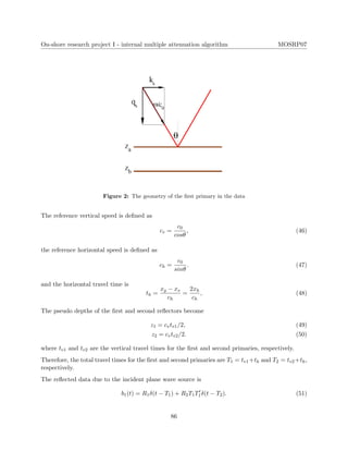
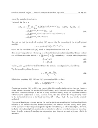
Suppose we choose the wrong reference velocity c0. The new vertical wave number becomes kz =
2ω/c0, and the new pseudo depths are za = c0t1/2 and zb = c0t2/2.
Equation (35) can be rewritten as
b1(z) = R1δ(z − za) + R2T1T1δ(z − zb). (39)
Substituting (44) into the third integral of (32), we have
∞
z2+
dz3eikzz3 [R1δ(z3 − za) + R2T1T1δ(z3 − zb)]
= R1eikzza
H(za − (z2 + )) + R2T1T1eikzzb
H(zb − (z2 + )),
(40)
where H is the Heaviside function. The second integral becomes
z1−
−∞
dz2e−ikzz2 [R1δ(z2 − za) + R2T1T1δ(z2 − zb)]
· [R1eikzza
H(za − (z2 + )) + R2T1T1eikzzb
H(zb − (z2 + ))]
= R2
1eikz(za−za)
H(za − (za + ))H((z1 − ) − za)
+ R1R2T1T1eikz(za−zb)
H(za − (zb + ))H(z1 − − zb)
+ R1R2T1T1eikz(zb−za)
H(zb − (za + ))H(z1 − − za)
+ R2
2T2
1 T1
2
eikz(zb−zb)
H(zb − (zb + ))H(z1 − − zb).
(41)
The underlined Heaviside function in (41) are zero due to H(< 0) = 0. The remaining third term
is
R1R2T1T1eikz(zb−za)
H(zb − (za + ))H(z1 − − za). (42)
Therefore,
b3IM (kz) =
∞
−∞
dz1eikzz1 [R1δ(z1 − za) + R2T1T1δ(z1 − zb)]
· [R1R2T1T1eikz(zb−za)
H(zb − (za + ))H(z1 − − za)]
= R2
1R2T1T1eikz(zb−za+za)
H(zb − (za + ))H(za − − za)
+ R1R2
2T2
1 T1
2
eikz(zb−za+zb)
H(zb − (za + ))H(zb − − za)
= R1R2
2T2
1 T1
2
eikz(2zb−za)
= R1R2
2T2
1 T1
2
ei(2ω/c0)(2c0t2/2−c0t1/2)
= R1R2
2T2
1 T1
2
eiω(2t2−t1))
.
(43)
Note that the underlined term H(− ) = 0, and H(> 0) = 1.
84

9. On-shore research project I - internal multiple attenuation algorithm MOSRP07
The result of (43) agrees with the estimation that uses true reference velocity (see equation (38).
One can see that the internal multiple estimation is independent of reference velocity. The different
reference velocities will change the pseudo depths and the corresponding vertical wavenumbers but
the total time of the predicted multiple remain accurate. In other words, even if we use a wrong
reference velocity to perform this algorithm, the internal multiples will be properly predicted.
However, the independence from the reference velocity is only true for the 1-D normal incidence
case. In the next section, we will show that using inaccurate reference velocity to process the
internal multiple algorithm may cause errors in the non-normal incidence case.
A 1.5D analytic example of internal multiple attenuation
We consider a 2-D layering model given by Nita and Weglein (2005) (see Figure 1). The velocity
changes across the interfaces located at z = za and z = zb where the velocities are c0, c1, and c2,
respectively. The sources and receivers are located at the measurement surface where the depth
z = 0.
Figure 1: The model for the 1.5D example
The data in the frequency ω domain can be written as
D(xh, 0; ω) =
1
2π
∞
−∞
dkh
R1 + T1R2T1eiν1(zb−za) + · · ·
iqs
eikzza
eikhxh
. (44)
where kz = qg + qs, kh = kg − ks, xh = (xg − xs)/2, and ν1 = q1g + q1s.
For the first primary (see Figure 2), we have
qs =
ω
c0
cosθ. (45)
85

10. On-shore research project I - internal multiple attenuation algorithm MOSRP07
Figure 2: The geometry of the first primary in the data
The reference vertical speed is defined as
cv =
c0
cosθ
, (46)
the reference horizontal speed is defined as
ch =
c0
sinθ
. (47)
and the horizontal travel time is
th =
xg − xs
ch
=
2xh
ch
, (48)
The pseudo depths of the first and second reflectors become
z1 = cvtv1/2, (49)
z2 = cvtv2/2. (50)
where tv1 and tv2 are the vertical travel times for the first and second primaries, respectively.
Therefore, the total travel times for the first and second primaries are T1 = tv1+th and T2 = tv2+th,
respectively.
The reflected data due to the incident plane wave source is
b1(t) = R1δ(t − T1) + R2T1T1δ(t − T2). (51)
86

11. On-shore research project I - internal multiple attenuation algorithm MOSRP07
Fourier transforming into the frequency ω domain gives
b1(ω) = R1eiωT1
+ R2T1T1eiωT2
= R1eiω(tv1+th)
+ R2T1T1eiω(tv2 +th)
= [R1ei( 2ω
cv
)(
cvtv1
2
)
+ R2T1T1ei( 2ω
cv
)(
cvtv2
2
)
]e
i( 2ω
ch
)(
chth
2
)
.
(52)
Equation (52) can be rewritten as
b1(kh, kz) = [R1eikzz1
+ R2T1T1eikzz2
]eikhxh
. (53)
Fourier transforming b1 over xh, we find
b1(kh, kz) = [R1eikzz1
+ R2T1T1eikzz2
]δ(kg − ks). (54)
Inverse Fourier transforming equation (53) over kz gives
b1(kh, z) = [R1δ(z − z1) + R2T1T1δ(z − z2)]δ(kg − ks) (55)
Substituting equation (55) into the third integral of equation (23), we have
∞
z2+
dz3eikzz3 [R1δ(z3 − z1) + R2T1T1δ(z3 − z2)]δ(k2 − ks)
= [R1eikzz1
H(z1 − (z2 + )) + R2T1T1eikzz2
H(z2 − (z2 + ))]δ(k2 − ks).
(56)
The second integral is
z1−
−∞
dz2e−ikzz2 [R1δ(z2 − z1) + R2T1T1δ(z2 − z2)]δ(k1 − k2)
·[R1eikzz1
H(z1 − (z2 + )) + R2T1T1eikzz2
H(z2 − (z2 + ))]δ(k2 − ks)
= R2
1eikz(z1−z1)
H(z1 − (z1 + ))H((z1 − ) − z1)δ(k1 − k2)δ(k2 − ks)
+ R1R2T1T1eikz(z1−z2)
H(z1 − (z2 + ))H((z1 − ) − z2)δ(k1 − k2)δ(k2 − ks)
+ R1R2T1T1eikz(z2−z1)
H(z2 − (z1 + ))H((z1 − ) − z1)δ(k1 − k2)δ(k2 − ks)
+ R2
2T2
1 T1
2
eikz(z2−z2)
H(z2 − (z2 + ))H((z1 − ) − z2)δ(k1 − k2)δ(k2 − ks).
(57)
The underline Heaviside functions are zero. The remaining third term is
[R1R2T1T1eikz(z2−z1)
H(z2 − (z1 + ))H((z1 − ) − z1)]δ(k1 − k2)δ(k2 − ks). (58)
Therefore,
b3(kh, kz) =
∞
−∞
dz1e−ikzz1 [R1δ(z1 − z1) + R2T1T1δ(z1 − z2)]δ(kg − k1)
·[R1R2T1T1eikz(z2−z1)
H(z2 − (z1 + ))H((z1 − ) − z1)]δ(k1 − k2)δ(k2 − ks)
= R2
1R2T1T1eikz(z2−z1+z1)
H(z2 − (z1 + ))H((z1 − ) − z1)δ(kg − k1)δ(k1 − k2)δ(k2 − ks)
+ R1R2
2T2
1 T1
2
eikz(z2−z1+z2)
H(z2 − (z1 + ))H(z2 − − z1)δ(kg − k1)δ(k1 − k2)δ(k2 − ks)
= R1R2
2T2
1 T1
2
eikz(2z2−z1)
δ(kg − k1)δ(k1 − k2)δ(k2 − ks)
(59)
87

12. On-shore research project I - internal multiple attenuation algorithm MOSRP07
where the underline term is zero.
The result for the b3 is
b3(kh, kz) =
∞
−∞
dk1
∞
−∞
dk2R1R2
2T2
1 T1
2
eikz(2z2−z1)
δ(kg − k1)δ(k1 − k2)δ(k2 − ks)
= R1R2
2T2
1 T1
2
eikz(2z2−z1)
δ(kg − ks)
= R1R2
2T2
1 T1
2
ei2(ω/cv)(2cvtv2/2−cvtv1/2)
ei(2ω/ch)(chth/2)
= R1R2
2T2
1 T1
2
eiω(2tv2−tv1)
eiωth
(60)
One can see that the result of equation (59) agrees with the expression of the actual internal
multiple,
IMactual = R1R2
2T1T1eiω(2tv2−tv1)
eiωth
, (61)
except for the extra factor of T1T1, which is always less than but close to 1.
If we pick a wrong reference velocity, c0, to perform the internal multiple algorithm, the new vertical
and horizontal velocities become cv =
c0
cosθ and ch =
c0
sinθ , respectively. The new pseudo depths are
z1 = cvtv1/2, (62)
z2 = cvtv2/2. (63)
where tv1 and tv2 are the vertical travel times for first and second primaries, respectively.
The horizontal travel time becomes
th =
xg − xs
ch
=
2xh
ch
. (64)
Subsituting equations (62), (63) and (64) into equation (59), we have
IMest = R1R2
2T2
1 T1
2
eiω(2tv2−tv1)
eiωth . (65)
Comparing equation (65) to (61), one can see that the pseudo depths varies when we choose a
wrong reference velocity, but the vertical traveltimes tv1 and tv2 remain unchanged. However, the
horizontal traveltime changes if we use a wrong reference velocity since the horizontal distance
between source and receiver is fixed. In other words, the error due to the wrong velocity occurs
in the horizontal direction so the total traveltime (T = (2tv2 − tv1) + th) may not be precisely
predicted.
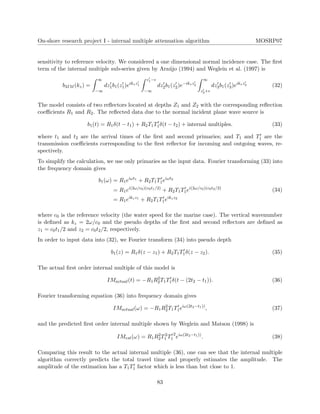
From the 1.5D analytic example, we find the inverse scattering series internal multiple algorithm is
sensitive to the reference velocity. In the marine case, the reference velocity, namely water speed,
is well-known so we have no problem predicting the correct timing of internal multiples. However,
in elastic internal multiple attenuation, the sensitivity to reference velocity becomes an important
issue. In order to properly perform the attenuation algorithm, an accurate reference velocity is
necessary.
88

13. On-shore research project I - internal multiple attenuation algorithm MOSRP07
Conclusion and Future Plan
This study showed that the inverse scattering series is a direct and effective method to predict inter-
nal multiples without any information below the measurement surface. However, four-component
data are needed to perform this algorithm effectively. Another requirement, the known reference
velocities, has effects on (P, S) decomposition and predicting the total traveltimes of internal mul-
tiples. We followed the analysis of Weglein and Matson (1998) and Nita and Weglein (2005) to
further investigate reference velocity sensitivity issue. The result revealed that velocity errors may
have an effect on predicting the correct timing of the interanl multiples for the 1D normal incidence
case. Therefore, this study will focus on the issue of reference velocity so that we can optimize the
performance of internal multiple attenuation for land data.
Acknowledgments
We are grateful to all M-OSRP sponsors for supporting our research. We also thank all the members
in M-OSRP for reviewing this manuscript and valuable discussions.
References
Ara´ujo, F. V. Linear and non-linear methods derived from scattering theory: backscattered tomog-
raphy and internal multiple attenuation. PhD thesis, Universidade Federal da Bahia, 1994.
Carvalho, P. M. Free-surface multiple reflection elimination method based on nonlinear inversion
of seismic data. PhD thesis, Universidade Federal da Bahia, 1992.
Matson, K. H. An inverse-scattering series method for attenuating elastic multiples from multi-
component land and ocean bottom seismic data. PhD thesis, University of British Columbia,
1997.
Nita, Bogdan G. and Arthur B. Weglein. Inverse scattering internal multiple attenuation algo-
rithm in complex multi-d media. Technical report, Mission-Oriented Seismic Research Project,
University of Houston, 2005.
Weglein, A. B., F. V. Ara´ujo, P. M. Carvalho, R. H. Stolt, K. H. Matson, R. T. Coates, D. Corrigan,
D. J. Foster, S. A. Shaw, and H. Zhang. “Inverse Scattering Series and Seismic Exploration.”
Inverse Problems (2003): R27–R83.
Weglein, A. B., F. A. Gasparotto, P. M. Carvalho, and R. H. Stolt. “An Inverse-Scattering Series
Method for Attenuating Multiples in Seismic Reflection Data.” Geophysics 62 (November-
December 1997): 1975–1989.
Weglein, A. B. and R. H. Stolt. I. The wave physics of downward continuation, wavelet estimation
and volume and surface scattering. II. Approaches to linear and non-linear migration inversion.
Mathematical Frontiers in Reflection Seismology. SEG/SIAM, 1995.
89

14. On-shore research project I - internal multiple attenuation algorithm MOSRP07
Weglein, Arthur B. and Ken H. Matson. “Inverse scattering internal multiple attenuation: an
analytic example and subevent interpretation.” SPIE, 1998, 108–117.
90